不確定TS模糊模型控制系統的強健穩定及二次有限時間最佳靜態輸出回授控制器設計研究

行政院國家科學委員會專題研究計畫 成果報告

不確定 TS 模糊模型控制系統的強健穩定及二次有限時間最

佳靜態輸出回授控制器設計研究

研究成果報告(精簡版)

計 畫 類 別 ： 個別型 計 畫 編 號 ： NSC 99-2221-E-151-009- 執 行 期 間 ： 99 年 08 月 01 日至 100 年 07 月 31 日 執 行 單 位 ： 國立高雄應用科技大學機械工程系 計 畫 主 持 人 ： 陳信宏 共 同 主 持 人 ： 鄭良安 計畫參與人員： 碩士班研究生-兼任助理人員：林銘修 碩士班研究生-兼任助理人員：羅易聖 報 告 附 件 ： 出席國際會議研究心得報告及發表論文 處 理 方 式 ： 本計畫涉及專利或其他智慧財產權，2 年後可公開查詢

中 華 民 國 100 年 09 月 05 日

1

行政院國家科學委員會專題研究計畫成果報告

不確定 TS 模糊模型控制系統的強健穩定及二次有限時間

最佳靜態輸出回授控制器設計研究

計畫編號：NSC99-2221-E-151-009

執行期限：99 年 8 月 1 日至 100 年 7 月 31 日

主 持 人：陳信宏 教授 國立高雄應用科技大學機械系

一、中英文摘要 本研究計畫報告係針對 TS 模糊模型動 態控制系統的二次有限時間最佳靜態輸出 迴授控制問題，來探討設計其最佳控制器的 研究課題。藉由田口基因演算法、正交函數 計算法，以及線性矩陣不等式技巧所推導出 的穩定性條件，來設計二次有限時間最佳靜 態輸出回授平行分配補償控制器。使用正交 函數計算法把不確定 TS 模糊模型動態控制 系統之二次有限時間靜態輸出回授平行分 配補償控制器設計的動態最佳化問題，轉換 成由代數方程式型態來表示的靜態最佳化 問題，以簡化設計的複雜度，再由田口基因 演算法的應用，配合強健穩定條件，共同來 解決閉迴路之不確定 TS 模糊模型動態控制 系統的二次有限時間最佳靜態輸出回授平 行分配補償控制器的設計問題。 關鍵詞：TS 模糊控制系統、二次最佳靜態 輸出回授控制、有限時間、正交函數計算 法、基因演算法、田口實驗設計法、線性矩 陣不等式。 Abstract

This report is to study the robust-stable and quadratic-finite-horizon-optimal design problems of the static output feedback parallel-distributed-compensation (PDC) controllers for TS fuzzy model systems with uncertain parameters. Firstly, a robust stabilizability condition is derived in terms of linear matrix inequalities (LMIs). By integrating the proposed stability condition, the orthogonal-functions approach (OFA) and the hybrid Taguchi genetic algorithm (HTGA) will be applied to solve the robust-stable and quadratic-finite-horizon-optimal static output

feedback controllers design problems for the uncertain TS fuzzy model systems. Based on the OFA, an algorithm only involving the algebraic computation for solving the TS fuzzy output feedback dynamic equations. By using the OFA, the quadratic finite-horizon optimal static output feedback PDC control problem for the TS fuzzy model systems is transformed into a static optimization problem represented by the algebraic equations; thus greatly simplifying the quadratic finite-horizon optimal static output feedback PDC control design problem. Then, for the static optimization problem, the HTGA can be easily employed to find the robust-stable and quadratic-finite-horizon-optimal static output feedback PDC controllers of the uncertain TS fuzzy model systems.

Keywords: static output feedback control, TS

fuzzy model, orthogonal-functions approach, hybrid Taguchi genetic algorithm, linear matrix inequalities.

二、計畫緣由與目的

It has been shown that the fuzzy-model-based representation proposed by Takagi and Sugeno (1985), known as the TS fuzzy model, is a successful approach for dealing with the nonlinear control systems. Unlike conventional modeling approaches where a single model is used to describe the global behavior of a nonlinear control system, the TS fuzzy modeling approach is essentially a multi-model approach in which the simple sub-models (typically linear models) are combined to describe the global behavior of the nonlinear control system. Each fuzzy rule for the TS fuzzy control system has a linear dynamic model as the consequent part which

expresses the local dynamics of each fuzzy rule. Then, the overall fuzzy model is achieved by blending these rules. The advantage of controller synthesis for such a fuzzy model is that the linear control methods can be used. There are many successful applications of the TS fuzzy model approach to the nonlinear control systems (see, Babuska, 1998; Farinwata et al., 2000; Tanaka and Wang, 2001; Tong et al., 2004; Chen et al., 2005; Xiu and Ren, 2005; Lian et al., 2006; Fang et al., 2006; Ho et al., 2007; Razavi-Panah and Majd, 2008; Lendek, et al., 2010). In practice, not all the state variables are accessible for control of dynamic systems. On the issue of choosing accessible measurements for feedback control of dynamic systems, the static output feedback control strategy would be the best choice because it is simple in controller structure (compared with the dynamic output feedback controller and the observer-based state feedback controller) and it is able to use the easily measureable variables as feedback signals to realize the control systems. Therefore, some researchers (Chang et al., 2003; Gong et al., 2004; Chen et al., 2005; Fang et al., 2006 ; Huang and Nguang, 2006, 2007 ; Wu, 2008; Soliman et al., 2009 ; Chang et al., 2009 ; Du and Zhang, 2009 ; Lee and Kim, 2009 ; Qiu et al., 2010 ; Chen et al., 2010 ; Jabri et al., 2010) have proposed some methods to design the static output feedback controllers of the TS fuzzy model systems.

2 On the other hand, in control systems design, it is often of interest to synthesize a quadratic-optimal controller such that the control objective of minimizing a quadratic integral performance criterion is achieved (Friedland, 1986; Goodwin et al., 2001). However, the problem of designing a quadratic-optimal static output feedback controllers is essentially very hard for the TS fuzzy model systems and, thus, rarely studied in the literature (Wu, 2008).

The purpose of this report is to propose an integrative numerical optimization method accompanied with the robust stabilizability condition to design the robust-stable and quadratic-finite-horizon-optimal static output feedback PDC controllers of the TS fuzzy model systems with elemental parametric

uncertainties. The method integrates the orthogonal-functions approach (OFA), the hybrid Taguchi-genetic algorithm (HTGA) and the linear-matrix-inequality (LMI) technique, where the LMI technique is used to derive the robust stabilizability condition for ensuring that the closed-loop uncertain TS fuzzy model systems can be robustly stabilized.

三、研究方法與成果

Based on the approach of using the sector nonlinearity in the fuzzy model construction, both the fuzzy set of premise part and the linear dynamic model with parametric uncertainties of consequent part in the exact TS fuzzy control model with parametric uncertainties can be derived from the given nonlinear control model with parametric uncertainties (Tanaka and Wang, 2001; Ho et al., 2007). The TS fuzzy model system with parametric uncertainties for the nonlinear control system with parametric uncertainties can be obtained as the following form:

i R~ : IF z1

( )

t is Mi1 and … and zg

( )

t is Mig, THEN

( )

_{( )}

( )

_{( )}

( )

⎩ ⎨ ⎧ Δ + = Δ + + Δ + = , )) ( ( , )) ( ( )) ( ( t x t C C t y t u t B B t x t A A t x i i i i i i & (1) with the initial state vector x

( )

0 , where R~i

(

i=1,2,_K,N

)

denotes the i-th implication, N is the number of fuzzy rules,

( ) ( ) ( )

[

( )

]

T t n 2 1t,x t, ,x x t

x = _K denotes the n-dimensional

state vector,

( )

[

( ) (

)

(

)

]

T 2 1t,y t, y = _K,y_r t t y denotes

the r-dimensional output vector,

( ) ( ) ( )

[

( )

]

T t p 2 1t,u t, ,u u t

u = _K denotes the p-dimensional

input vector, zi

( )

t

(

i=1 K,2, ,g

)

are the premise

variables, and are,

respectively, the , i A i Ci 2K, , n n B

(

i=1, ,N

)

× n×p and r×n

consequent constant matrices, ΔAi(t), ΔBi(t) and ΔCi(t)

(

i=1, K2, ,N

)

are, respectively, the time-varying parametric uncertain matrices existing in the system matrices the input matrices and the output matrices of the consequent part of the i-th rule due to the inaccurate measurement, inaccessibility to the system parameters, output-sensor measurement variations, or variation of the

parameters, and and

, i A , 2 , 1 = i B C_i N ij M

(

i _K,

)

g j=1,2,_K,

( )

t , Ai Δ ΔBi

(

t

( )

1

∑

= = Δ m q i t A ε

( )

= ΔC_i t

( )

t iq

are the fuzzy sets.

_[

∑∑∑

= = = = N i N j N l ijl l j i z t h z t h z t A h t x 1 1 1 )) ( ( )) ( ( )) ( ( ) ( &

( )

( )

∑

∑

= = + + m q m q ijlq lq ijlq iqtE t F 1 1 ε ε

We suppose that the time-varying elemental parametric uncertain matrices

and take the forms

)

ΔCi(t)

( )

_iq, iq t A

( )

( )

, 1

∑

= = Δ m q iq iq i t t B B ε

_{( )}

_{( )}

_{( )}

, 1 1 t x G t t m q ijlqs m s ls iq ⎥ ⎦ ⎤ +

∑

∑

= = ε ε (6) and

( )

, (2) 1

∑

= m q iq iq tC ε where , l j i i ijl A BFC A = + (7a)

where ε

(

εiq ≤εiq

( )

t ≤εiq

)

are the time-varying elemental parametric uncertainties, and and are, respectively, the given

, iq A n iq B , n iq C × n×p and r×n

constant matrices which are prescribed a priori to denote the linearly dependent information on the time-varying elemental parametric uncertainties εiq

( )

t , in which and N , K i=1,2, . m , , l j iq iq ijlq A B FC E = + (7b) , lq j i ijlq BFC F = (7c) and . ls j iq ijlqs B FC G = (7d) 3 , 2 , 1 q= _K

∑

= = N i i zt h t x 1 )) ( ( ) ( & ( ) ( 1

∑

= = N i i z h t y

The resulting uncertain TS fuzzy model system inferred from Eq. (1) is represented as

[

(A_i+ΔA_i(t))x(t)+(B_i+ΔB_i(t))u(t)

]

(3)

For the closed-loop uncertain TS fuzzy model system in Eq. (6), the problem of robust stabilizability analysis is, under the condition that the local static output feedback gain matrices Fi

(

i=1,2,K,N

)

of the static

output feedback PDC controller in Eq. (5) have been specified in advance, to derive a robust stabilizability criterion for checking whether the closed-loop uncertain TS fuzzy model system in Eq. (6) can be robustly stabilized by the specified static output feedback PDC controller or not.

and (4)

[

( ( )) ( )

]

, )) (t Ci+ΔCi t x t in which

( )

[

( ) ( )

( )

]

T 2 1t ,z t , ,z t z t = K g

)

( )

( )

z

( )

( )

( )

(

denotes

the g-dimensional premise vector,

,

1

∑

=

Theorem:

The closed-loop uncertain TS fuzzy model system in Eq. (6) is robustly stabilizable, if, for the specified local static output feedback gain matrices Fj

(

j=1,2,_K,N

)

in Eq. (5), there exists a symmetric positive definite matrix P such that the following LMIs are simultaneously satisfied: = _i i zt w zt h

( )

N i i zt w and

( )

( )

( )

( )

, 1

∏

= = g j j ij i zt M z t w

( )

z t Mij j

( )

t zj , 2 , 1 j= _K

( )

( )

z t ≥0 hi

∑

= = N i i z h t u 1 ( ( ) ( ( 1 1

∑∑

= = = N i N j i h i F i

are the grades of membership of in the fuzzy sets

and It can be seen that, for all t, and ij M

(

i=1,2,_K,N . 1 =

)

. , g

( )

( )

1

∑

= N i i zt h

(

Sijle+Uijlf+ViwFjWlh

)

TP+P

(

Sijle+Uijlf+ViwFjWlh

)

<0, (8) The following static output feedback

PDC controller is considered here: where

( )

_{( )} , or 0 ijlq iqt iq iq m q iq ijle t E S ε ε ε ε ₌ =

∑

= (9)

[

Fiy t t)) () )) ( ( )) (t hj zt z

]

)

(5)

[

Fi(Cj+ΔCj(t))x(t)

]

,

( )

( ) or , 1 ijlq lqt lq lq m q lq ijlf t F U ε ε ε ε ₌ =

∑

= (10)

where

(

=1,2,_K,N denote the p×r

local static output feedback gain matrices.

( )

_{( )} or ,

1 iq iqt iq iq m q iq iw t B V ε ε ε ε ₌ =

∑

= (11) By substituting Eqs. (2) and (5) into Eq.

(3), we can get the closed-loop uncertain TS

fuzzy model system as

( )

( ) or ,

1 lq lpt lq lq m q lq lh tC W ε ε ε ε ₌ =

∑

= (12) ijl ijl A E 0= and εi0

( )

t =εi0 =εi0 =1, for

N l j i, , =1,2,_K, i F

(

i=1,2,_K,

∑

= = N i i h t x 1 ( ) ( & ( ) ( 1

∑

= = N i i h t y ) ( 1 1

∑∑

= = = N i N j i h t u

( )

and , , , 1,2, ,2m. h w f e = _K

)

[

Aix(t)+Biu(t)

]

[

C_ix(t)

]

,

[

( )

]

, )) ( ( i j j z t FC x t h

( ) ( )

[

]

However, only robust stabilizability is often not enough in control design. The control objective of minimizing a quadratic finite-horizon integral performance criterion for the nominal dynamic systems is also considered in many practical control engineering applications (Friedland, 1986; Goodwin et al., 2001). On the other hand, before we are able to synthesize a controller such that the good control performance for a given dynamic system can be efficiently achieved, it is necessary that the given dynamic system can be stabilized by the controller (Nise, 2000; Yu, 2002). In addition, both optimality and stability should be simultaneously considered in the optimal controllers design (Skelton, 1988). Therefore, the problem considered here is how to specify the local static output feedback gain matrices of the static output feedback PDC controller in Eq. (5) such that the constraint of LMI-based robust stabilizability condition in Eq. (8) for the closed-loop uncertain TS fuzzy model system in Eq. (6) can be satisfied, and such that the optimal control performance for the nominal TS fuzzy model system

N 4 t z ))( (13) and z(t)) (14) where ( tz( )) (15)

can be achieved by minimizing the following H2 quadratic finite-horizon integral performance index:

( )

∫

+ = qtf u t y Q t y J 0 T dt t u R t T

( )

( ) ( )

[

( )

( )

_]

, T +u t Rut dt t y 1 0 1 T

∑∫

₌− + = q k t k t k y t Q f f (16) where denotes a small time interval which is chosen for the independent variable t,

f

t

q is

a positive integer specified by the designer, Q is a symmetric positive-semidefinite matrix, and R is a symmetric positive-definite matrix.

Here the time interval of interest is designated as being from t=0 to t=qt_f, where t=0

is the initial time and t=qtf is the final time

of the control period.

The problem to be studied here can be named the mixed H2/LMI static output feedback PDC controllers design problem of the uncertain TS fuzzy model systems, and the design procedures for the static output feedback PDC controllers can be described as following:

Step 1: Check the constraint of

LMI-based robust stabilizability condition in Eq.

(8).

Step 2: Minimize the H2 quadratic

finite-horizon integral performance index in Eq. (15)

for the nominal TS fuzzy model system in Eqs. (13) and (14). That is, the design problem of the mixed H2/LMI static output feedback PDC controllers for the uncertain TS fuzzy model systems is a constrained dynamic optimization problem. We will integrate the OFA, the HTGA and the presented LMI-based robust stabilizability condition to solve the mixed H2/LMI static output feedback PDC controllers design problem of the uncertain TS fuzzy model systems, where the performance index subject to the constraint of robust stabilizability condition is considered to be directly minimized.

Here, consider the time interval , f ) 1 ( f t k t t

k ≤ ≤ + where is chosen for the

independent variable t, and let us define f t (17) , η + = tk t f and

( )

kt_f , (18) k x x = in which k =0,1,2,_K,q−1, and 0≤η≤tf. The state vector x

( )

t , within

(

1

)

f t k t

t

k ≤ ≤ + _f, can be approximated by the

truncated orthogonal-functions representation as

( )

1 ( )

( )

~( )

( )

_, 0

∑

− = = =m s k s k s T t x T t x t x (19)

where m is the number of terms required for

the OF,

( )

[

( ) ( )

( )

]

T 1 1 0 t ,T t , ,T t T t T = K m− denotes

the m×1 OF basis vector, Ti

( )

t

(

i=0,1,_K,m−1

Now, if one set of local output feedback gain matrices

{

F1,F2,K,FN

}

is given, then

( )k x

~

₍

_{k =0,1,K,q−1}

₎

_{can be calculated from} the following algorithm only involving the algebraic computation.

)

denote the OF, ( )k s

x

(

s =0,1,_K,m−1

)

are the coefficient vector, and 1 × n ( )

[

( ) ( ) ( )k

]

m 1− is k k k x x x 0 , 1 ~ _{= ,K,x the} m n× coefficient matrix of x

( )

t .

( )

t x ( ) T ₊ j i k CQC

( )

k i lz A h

Detailed Steps: Algebraic Algorithm

Substituting Eqs. (14) and (15) and the truncated OF representation of in Eq. (19) into the quadratic integral performance index in Eq. (16), the quadratic integral performance index J becomes the following algebraic form:

Step 1: Give a small time interval

the specified positive integer q, and the initial state vector

, f t

( )

0 , x and set k =0.

Step 2: Calculate hi

(

z

( )

ktf

)

for

( ) ( )~ ( ) ( ) ( ) ( ) trace 1 0 1 1 1 1 T T T ∑− ∑∑∑∑ = ⎢ = = = = ⎢ ⎣ ⎡ ⎟⎟ ⎠ ⎞ ⎜⎜ ⎝ ⎛ =q k N i N j N l N o o l i j o k l k j k i k C F R F C h z h z h z h x W J ( )~( ) , ⎥ ⎥ ⎦ ⎤ k x ( )k _, H z

)

,

( )

k . , , 2 , 1 N i= _K

(20) _{Step 3: Calculate} ( )k _{from Eq. (24).} xˆ

where the constant matrix W is the product-integration-matrix of two OF basis vectors (Ho and Chou, 2007).

Step 4: Compute xk+1 by using

(

)

(

₁

)

~( )

(

(

₁

)

)

_. 1 f k f k x k t x T k t x + = + = +

Step 5: Set k= k+1. If k> q−1, then

stop; otherwise go to Step 2. Using the following integral property of

the OF:

From the above algorithm, it is obvious that if one set of local static output feedback gain matrices

{

F1,F2,K,FN

}

is specified, then ( )k

x

~

₍

_{k=0,1,K,q−1}

₎

_{can be determined,} and thus the value of the performance index in Eq. (20) corresponding to this set of

{

F ,1 F2,K,FN

}

can be calculated. Given another set of local static output feedback gain matrices

{

F₁,F₂,_K,F_N

}

,

1 F

there obtains another value of the performance index in Eq. (20). That is, the value of the performance index of algebraic form in Eq. (20) is actually dependent on the set of local static output feedback gain matrices which means

{

,F₂,_K,F_N

}

,

( )

t dt HT

(

t T t t k f =

∫

(21) applying Eqs. (18) and (19), and following the same procedures as those in the previous works of the authors (Ho et al., 2007, 2009), Eq. (13) with Eqs. (14) and (15) can be cast into the form

( )

_[

_{,0,0, ,0}

_]

_{( )}

(

)

~ ~ 1 1 1

∑∑∑

= = = − = − N i N j N l l j i j k i k k x C F B z h z h x x _K (22) in which H is the operational matrix of integration for the OF (Ho et al., 2007, 2009),

( )

_{k i}

(

( )

_f

)

, i z h z kt h = and k =0, 1, 2,_K, q−1.

(

)

~( )k l jC x F

]

Eq. (22) can be rewritten as

( )

( ) ( ) ( )

~( )_, ~ 1 1 1 k N i N j N l i k l k j k i k Q H B A z h z h z h x −

∑∑∑

− = = = = (23)

(

f₁₁₁, f₁₁₂, , f_Npr

)

, G J = _K (25) i where ~( )

[

,0,0, ,0 5 K k k x Q = is an n×m matrix.

Making use of the Kronecker product, the explicit form for the coefficient matrix

( )k x

~ _{comes directly from Eq. (23) as}

( )

_{( ) ( ) ( )}

(

T

(

)

i A− ⊗

)

_ˆ( ) ˆ 1 1 1 1 k N i N j N l l j i k l k j k i n m k Q C F B z h z h z h I x − = = = ⎥⎦ ⎤ ⎢ ⎣ ⎡ − =

∑∑∑

(24) , H where n m

I denotes the mn×mn identity matrix, ( )

[

( ) _, ( ) _{, ,} ( )

]

_, ˆ ₀ T ₁ T k₁T T m k k k x x x x = K −

and denotes the Kronecker product (Barnett, 1979). This implies that

( ) T_, k k x =

[

0T,0T, ,0T T, K ( )k x

]

where fijk

(

i=1,2,K,N, j=1,2,K, p and

)

k=1,2,_K,r denote the elements of the local

static output feedback gain matrices Hence, the design problem of the robust-stable and quadratic-finite-horizon-optimal static output feedback PDC controller for the uncertain TS fuzzy model system is to search for the optimal such that there exists a symmetric positive definite matrix P to make the LMIs in Eq. (8) hold, and such that the performance index of algebraic form in Eq. (20) for the nominal TS-fuzzy-model-based dynamic system in Eqs. (13) and (14) is minimized. This is equivalent to the static

. i F ijk f ˆ Q ⊗ ~ _{can be} obtained from Eq. (24).

constrained-optimization problem

min J =G

(

f111, f112,K, fNpr

)

(26) subject to f_ijk ≤C~_ijk, and subject to the constraint that there exists a symmetric positive definite matrix P to make the LMIs in Eq. (8) hold, for

and where , , , 2 , 1 N i= _K ijk C p j=1,2,_K, , , , 2 , 1 r

k= _K ~ are the positive

real numbers given from the practical consideration, respectively. This means that, by using the OFA and the LMI-based robust stabilizability condition, the robust-stable and quadratic-finite-horizon-optimal static output feedback PDC control problem for the uncertain TS fuzzy model systems can be replaced by a static constrained-optimization problem represented by the algebraic equations with constraints; thus greatly simplifying the robust-stable and quadratic-finite-horizon-optimal static output feedback PDC control problem. Then, the HTGA can be employed to search for the optimal solution of the static constrained-optimization problem in Eq. (26), where Eq. (26) is a nonlinear function with the continuous variables. The detailed steps of the HTGA can be found in the works of Tsai et al., (2004, 2006). 6 四、研究成果自評 本成果報告已達成申請計畫書中預期 完成的成果目標。本研究計畫案之部份成果 的發表情況如下所列：

1. W. H. Ho, S. H. Chen, J. H. Chou, and C. C. Shu, “Design of Stable and Quadratic-Optimal Static Output Feedback Controllers for TS-Fuzzy-Model-Based Control Systems: An Integrative Computational Approach”, International

Journal of Innovative Computing, Information and Control, 2011 (in press).

2. W. H. Ho, S. H. Chen, J. H. Chou, and C. C. Shu, “Optimal Static Output Feedback Control of Fuzzy-Model-Based Control Systems”, Proc. of the 2011 IEEE

International Conference on Fuzzy Systems, pp.1774-1777, June 2011, Taipei,

Taiwan.

3. S. H. Chen, W. H. Ho, J. H. Chou and C. W. Li, “Robust-Stable and Quadratic-

Optimal Static Output Feedback Control for Uncertain Fuzzy Model Systems”, 2011 (submitted to International Journal). 五、參考文獻

1. Babuska, R., 1998, Fuzzy Modeling for Control, Kluwer, Boston.

2. Barnett, S., 1979, Matrix Methods for Engineers and Scientists, McGraw-Hill, New York.

3. Chang, W., J. B. Park, Y. H. Joo and G. Chen, 2003, “Output feedback fuzzy control for uncertain nonlinear systems”, ASME J. of Dynamic Systems, Measurement and Control, Vol. 125, pp. 521-530.

4. Chang, X. H., G. H. Yang, and X. P. Liu, 2009, “H∞ fuzzy static output feedback control of T-S fuzzy systems based on fuzzy Lyapunov approach”, Asian J. of Control, Vol. 11, pp. 89-93.

5. Chen, S. S., Y. C. Chang, S. F. Su, S. L. Chung, and T. T. Lee, 2005, “Robust static output-feedback stabilization for nonlinear discrete-time systems with time delay via fuzzy control approach”, IEEE Trans. on Fuzzy Systems, Vol. 13, pp. 263-272.

6. Chen, J., F. Sun and C. Hu, 2010, “Fuzzy H∞ control for nonlinear systems via static output feedback”, Proc. of the 7th International Conference on Fuzzy Systems and Knowledge Discovery, Yantai, China, Vol. 2, pp. 871-875 7. Du, H. and N. Zhang, 2009, “Static output

feedback control for electrohydraulic active suspensions via T-S fuzzy model approach”, ASME J. of Dynamic Systems, Measurement and Control, Vol. 131, pp. 1-11.

8. Fang, C. H., Y. S. Liu, S. W. Kau, L. Hong and C. H. Lee, 2006, “A new LMI-based approach to relaxed quadratic stabilization of T-S fuzzy control systems”, IEEE Trans. on Fuzzy Systems, Vol. 14, pp. 386-397.

9. Farinwata, S. S., D. Filev and R. Langari, 2000, Fuzzy Control: Synthesis and Analysis, John Wiley and Sons, Chichester.

10. Friedland, B., 1986, Control System Design: An Introduction to State-Space Methods, McGraw-Hill, New York.

11. Gong, C. Z., Q. L. Liu and W. Wang, 2004, “Static output feedback stabilization of uncertain fuzzy systems with time-delay: an iterative linear matrix inequality approach”, Control Theory and Applications, Vol. 21, pp. 627-630.

12. Goodwin, G. C., S. F. Graebe and M. E. Salgado, 2001, Control System Design,

7 Prentice-Hall, New Jersey.

13. Ho, W. H. and J. H. Chou, 2007, “Design of optimal controller for Takagi-Sugeno fuzzy model based systems”, IEEE Trans. on Systems, Man and Cybernetics, Part A, Vol. 37, pp. 329-339.

14. Ho, W. H., J. T. Tsai and J. H. Chou, 2007, “Robust-stable and quadratic-optimal control for TS-fuzzy-model-based control systems with elemental parametric uncertainties”, IET Control Theory and Applications, Vol. 1, pp. 731-742.

15. Ho, W. H., J. T. Tsai and J. H. Chou, 2009, “Robust quadratic-optimal control of TS-fuzzy-model-based dynamic systems with both elemental parametric uncertainties and norm-bounded approximation error”, IEEE Trans. on Fuzzy Systems, Vol. 17, pp. 518-531.

16. Huang, D. and S. K. Nguang, 2006, “Robust static output feedback control of fuzzy systems: an ILMI approach”, IEEE Trans. on Systems, Man, and Cybernetics, Part B, Vol. 36, pp. 216-222.

17. Huang, D. and S. K. Nguang, 2007, “Static output feedback controller design for fuzzy systems: an ILMI approach”, Information Sciences, Vol. 177, pp. 3005-3015.

18. Jabri, D., K. Guelton and N. Manamanni, 2010, “Decentralized static output feedback control of interconnected fuzzy descriptors”, Proc. of the 2010 IEEE International Symposium on Intelligent Control, Tokyo, Japan, pp. 117-122. 19. Lee, H. J. and D. W. Kim, 2009, “Robust

stabilization of T-S fuzzy systems: fuzzy static output feedback under parametric uncertainty”, Int. J. of Control, Automation and Systems, Vol. 7, pp. 731-736.

20. Lee, H. J. and D. W. Kim, 2009, “Fuzzy static output feedback may be possible in LMI framework”, IEEE Trans. on Fuzzy Systems, Vol. 17, pp. 1229-1230.

21. Lendek, Z., J. Lauber, T. M. Guerra, R. Babuska and B. De Schutter, 2010, “Adaptive observers for TS fuzzy systems with unknown polynomial inputs”, Fuzzy Sets and Systems, Vol. 161, pp. 2043-2065.

22. Lian, K. Y., J. J. Liou, and C. Y. Huang, 2006, “LMI-based integral fuzzy control of DC-DC converters”, IEEE Trans. on Fuzzy Systems, Vol. 14, pp. 71-80.

23. Nise, N. S., 2000, Control Systems Engineering, John Wiley and Sons, New York. 24. Qiu, J., G. Feng and H. Gao, 2010, “Output

feedback control of nonlinear systems under unreliable communication links via T-S fuzzy

models”, Proc. of the 8th IEEE International Conference on Control and Automation, Xiamen, China, pp. 2036-2041.

25. Razavi-Panah, J. and V. J. Majd, 2008, “A robust multi-objective DPDC for uncertain T-S fuzzy systems”, Fuzzy Sets and Systems, Vol. 159, pp. 2749-2762.

26. Skelton, R. E., 1988, Dynamic Systems Control, John Wiley and Sons, New York. 27. Soliman, M., A. L. Elshafei, F. Bendary and

W. Mansour, 2009, “LMI static output-feedback design of fuzzy power system stabilizers”, Expert Systems with Applications, Vol. 36, pp. 6817-6825.

28. Takagi, T. and M. Sugeno, 1985, “fuzzy identification of systems and its applications to modeling and control”, IEEE Trans. on Systems, Man and Cybernetics, Vol. 15, pp. 116-132.

29. Tanaka, K. and H. O. Wang, 2001, Fuzzy Control Systems Design and Analysis: A Linear Matrix Inequality Approach, John Wiley and Sons, New York.

30. Tong, S. C., T. Wang, Y. P. Wang and J. T. Tang, 2004, Design and Stability Analysis of Fuzzy Control Systems, Science Press, Beijing.

31. Tsai, J. T., T. K. Liu and J. H. Chou, 2004, “Hybrid Taguchi-genetic algorithm for global numerical optimization”, IEEE Trans. on Evolutionary Computation, Vol. 8, pp. 365-377.

32. Tsai, J. T., J. H. Chou and T. K. Liu, 2006, “Tuning the structure and parameters of a neural network by using hybrid Taguchi-genetic algorithm”, IEEE Trans. on Neural Networks, Vol. 17, pp. 69-80.

33. Wu, H. N., 2008, “An ILMI approach to robust H2 static output feedback fuzzy control

for uncertain discrete-time nonlinear systems”, Automatica, Vol. 44, pp. 2333-2339.

34. Xiu, Z. H. and G. Ren, 2005, ‘Stability analysis and systematic design of Takagi-Sugeno fuzzy control systems”, Fuzzy Sets and Systems, Vol. 151, pp. 119-138. 35. Yu, L., 2002, Robust Control: Linear Matrix

Inequality Approach, Tsinghua University Press, Beijing.

國科會補助專題研究計畫項下出席國際學術會議心得報告

日期： 100 年 7 月 15 日

計畫編號 NSC 99－2221－B－151－009

計畫名稱

不確定 TS 模糊模型控制系統的強健穩定及二次有限時間最佳靜態輸出

回授控制器設計研究

出國人員

姓名

陳信宏

服務機構

及職稱

國立高雄應用科技大學機械工程系

教授

會議時間

100 年 7 月 10 日

至

100 年 7 月 13 日

會議地點

中國大陸桂林

會議名稱

(中文)2010 年機器學習與控制國際研討會

( 英 文 )The 2011 International Conference on Machine Learning and

Cybernetics (ICMLC2011)

發表論文

題目

(中文)應用改善型微分進化法則之最佳預測模式

(英文) Optimal Prediction Model Using Improved Differential Evolution

Algorithm

一、參加會議經過：

本 屆 2010 年 機 器 學 習 與 控 制 國 際 研 討 會 (The 2011 International Conference on

Machine Learning and Cybernetics)是由國際電機電子工程師學會(IEEE)所主辦的年度盛

會，地點在中國大陸桂林Sheraton Guilin Hotel舉行，自2011年7月10日至7月13日為期四

天。我與研究團隊於2011年7月8日搭乘華航航空公司班機，由高雄小港國際機場飛抵香

港國際機場，再轉機南方航空公司班機至中國大陸桂林國際機場，搭巴士至Sheraton

Guilin Hotel參加會議。我與研究團隊住宿於桂林灕江瀑布大酒店以方便開會。

今年會議接受發表之口頭論文與壁報論文共有362篇，作者來自中國大陸、香港、

澳門、美國、義大利、澳洲、巴基斯坦、伊朗、泰國、英國、日本、孟加拉、土耳其以

及台灣共14個國家的研究學者共同參與。362篇論文中，大都來自亞洲國家的研究學者，

台灣研究學者參與發表論文僅次於中國大陸，可見台灣的研究能量逐漸的提升，在亞洲

佔有很重要的地位。除論文發表外，會議中也有3場邀請演講，我參加其中一場，由中

國大陸的學者Seong-Whan Lee演講機器學習對腦科學的挑戰，說明了機器學習未來的發

展。會議論文研討課題非常豐富，包括：智慧型系統與控制、智慧型多媒體應用、虛擬

影音應用、模糊理論與方法、影像處理、智慧服務系統、類神經網路、資料探勘、文字

探勘、數值最佳化、模型建模與模擬、與……等等，涵蓋了機器學習、智慧型控制之理

論、技術、和應用等各個層面。在會議期間，我們參加的論文發表場次以人工智慧、機

1

2

器學習等課題為主，經過參與討論及交換心得，我們深感獲益良多。

我與研究團隊的論文“Optimal Prediction Model Using Improved Differential Evolution

Algorithm”被安排在7月11日上午之口頭報告論文的場次”Intelligent Systems and Control”

中發表，在會議中有多位學者提出問題和我們討論，彼此交換心得，使我們獲益匪淺。

二、與會心得：

各國的學者專家共聚一堂，彼此交換研究心得，發表新的研究成果，參與此次國際

會議以及在中國大陸桂林的所見所聞，讓我們收獲良多，而且也有下列幾點心得：

(1) 人工智慧與機器學習的應用越來越廣泛與純熟，對醫學與生物領域而言，將是研究

之一大趨勢。台灣在此方面之研究應加以重視。

(2) 從各國發表之論文，可發現台灣學者的研究越來越多樣性，在實務上的應用也越來

越廣泛。

(3) 亞洲國家的研究學者參加國際研討會的人數非常多，台灣學者也越來越重視國際交

流，這是可喜的現象。

三、建議：

建議國科會與教育部提供更多學者出席國際會議之經費與名額(包括提供經費與名

額，給未獲得國科會研究計畫案的學者)，以培養國際觀，增強台灣在國際學術界的活絡

人脈和國際合作。

四、攜回資料名稱及內容：

攜回 ICMLC 2011 論文集之 CD 乙片，內容有此次國際研討會所發表的全部論文；

以及會議議程手冊乙本，內容有全部論文的摘要。

Optimal Prediction Model Using Improved Differential Evolution

Algorithm

Ming-Chang Zheng 1,Jyh-Horng Chou 1

, and Shinn-Horng Chen 2 1

Institute of Engineering Science and Technology National Kaohsiung First University of Science and Technology

2

Department of Mechanical Engineering, National Kaohsiung University of Applied Sciences, Taiwan

Abstract

A Taguchi-based the differential evolution (TDE) is applied as an improved the differential evolution to solve the global optimization. The differential evolution (DE) is an easy and valid evolutionary algorithm for fitness function optimization. For grey forecasting model (GM) which is a time series forecasting model, the parameters are calculated by the TDE. The academic research of Wang and Hsu is a base of this paper. Finally, the forecasted result of TDEGM is superior to other evolutionary algorithms.

Keywords ： Grey forecasting model; Evolution algorithm; Optimal

1. Introduction

Grey system theory is proposed by Deng[1].The past decades have seem growing importance placed on research in grey forecasting. The grey method has been widely used for the forecasting. The grey model is characterized by exceptionally high accuracy of predicted value with only a few data. Grey theory is widely applied in many applications. In this paper, a method using Taguchi-differential evolution algorithm (TDE) is presented to improve the accuracy of the original GM(1,1) model. The foundations of this research are grounded on the academic research of

Wang and Hsu [2]. Furthermore, in this study, the outputs of the integrated circuit industry of Taiwan is used as our example to examine the model reliability and accuracy. According to the forecasting presented in this paper, Taguchi-differential evolution algorithm Grey method(1,1)(TDEGM(1,1)) seems to be the best method for forecasting integrated circuit industry of Taiwan.

2. Methodology

The Grey Method(1,1), proposed by Deng[1] , is an effective mathematical means to deal with systems forecasting characterized by deficient information. The GM(1,1) model is a time series model.

The normal differential equation of GM(1,1)model is

( )

_{( )}

, ) 1 ( ) 1 ( b t aX dt t dx _{+ =} (1) where t denotes the independent variables in the system , a represent the developed coefficient, b is the grey controlled variable, and a and b denote the parameters need to be determined in the model. The

original data sequence denoted by

) 1 ( ) 0 ( x , (0)(2)

x ,….and x(0)(n) are used to construct the grey forecasting model and accurately predict

)..., 2 ( ), 1 ( (0) ) 0 ( _{n+ x n+} x and x(0)(n+k). The

)) ( ,..., 2 ( ), 1 ( ) ( (0) (0) (0) ) 0 ( n x x x k x =

{

(0)( ); 1,2,3...,

}

. n K k x = = (2)

When a model is constructed, the grey system must apply one-order accumulated generating operation (AGO) to the primitive sequence in order to provide the middle message of building a model and to weaken the variation tendency. Hereupon, x(1)(1) is defined as (0)(1)

x to be one-order AGO sequence. That is,

( )

. ) ( ,..., ) ( , ) ( )} ( { 1 ) 1 ( 2 1 ) 1 ( 1 1 ) 1 ( ) 1 ( ) 0 (       = =

∑

∑

∑

= = = n k k k k x k x k x k x k x AGO (3)

From Eqs.(1) and (3) and the ordinary least-square method, the coefficient

∧ a becomes . ) ( 1 N T T Y B B B b a a − ∧ =       = (4)

Additionally, the accumulated matrix B is

[

]

[

]

[

]

             + − − + − + − = 1 ) ( ) 1 ( 5 . 0 1 ) 3 ( ) 2 ( 5 . 0 1 ) 2 ( ) 1 ( 5 . 0 ) 1 ( ) 1 ( ) 1 ( ) 1 ( ) 1 ( ) 1 ( n x n x x x x x B ⋮ ⋮ .

Improved grey GM(1,1) forecasting model YN is

. ) ( ) 4 ( ) 3 ( ) 2 ( ) 0 ( ) 0 ( ) 0 ( ) 0 (                 − − − − = n x x x x YN ⋮ (5)

Here, both parameters (a,b) of GM(1,1) model can be obtained by the minimum least square estimation[1]. The original forecasting equation of GM(1,1) is denoted as below: a b e a b x k x ak ₊     ₋ = + − ∧ ) 1 ( ) 1 ( (0) 0 , where k=2,3,….,n.

When the sequence one-order

inverse-accumulated generating operation(IAGO) is acquired, the sequence can be obtained as the following: ). ( ) 1 ( ) 1 ( ) 0 ( ) 1 ( ) 0 ( k x k x k x ∧ ∧ − + = + (6)

Given k=1,2,.…n, the sequence of reduction is obtained as following: , ) 1 ( ),..., 1 ( ), 2 ( ), 1 ( ) 0 ( ) 0 ( ) 0 ( ) 0 ( ) 0 (       ₊ = ∧ ∧ ∧ ∧ ∧ n x x x x x (7) where ( 1) ) 0 ( + ∧ n

x is the Grey elementary predicting value of (0)( ₊1)

n x .

3. Improved grey GM(1,1) forecasting model

This section describes the proposed DEA approach. The detailed steps are as follows.

A. Population Initialization

The DEA is started with generating a population of real-valued D-dimensional vectors

G _min ( _{max min}) i

X =X +β X −X , (8) where G

i

X denotes the ith population vector in the G generation i=1 ⋯,2, ,NP, Xmin and Xmax are lower

bound and upper bound, respectively, and β is random number, where β∈[ ]0,1 .

B. Mutation by the Taguchi-method.

Mutation is an operation that adds a vector differential to a population vector. In this approach, a perturbed vector _VG+1

i is generated according to the

following form:

(

G

)

r G r G r G r G best F X X X X X _{1 2 3 4} 1 G i V + = + + − − , (9) where r1,r2,r3,r4∈[0,NP−1], and G best X is the best performing vector of the current generation.

In this study, r1,r2,r3,r4 are chosen randomly for

the interval [0,NP-1] and are different. F is a real and

scaling factor, where F ∈[ ]0,2 , which controls the amplification of the differential variation. In this study the Taguchi method is used to choose the best perturbed vector _VG+1

i . Below, we describe these steps.

Algorithm:

Step1: Set the fitness function. For reducing the

forecasting error, this study sets the fitness function as: Minimize: MAPE 100% (( ˆ )/ ) 1

∑

= − × = n i i i i n y y y

The Mean Absolute Percentage Error (MAPE), average of absolute values of all the

percentage errors, over the sample period can be used to find out the most model level. Like the other cost function, for the MAPE lower values are better. The yt

∧

is the predicted value, and yt is the actual value.

Step2: Select four-level of two-level of r₁,r₂,r₃,r₄ in Eq.(9) by using roulette wheel approach, respectively.

Step3: Select a suitable orthogonal array for matrix

experiments.

Step4: Calculate the values of perturbed vector 1

VG+ i

of n experiments in the orthogonal array.

Step5: One optimal chromosome, which is new

perturbed vector 1

VG+

i , is generated based on

the results from step3.

Step6: Repeat Step1 through 4 until i = NP. This step

will produce NP perturbed vectors. C. Crossover

In order to increase the diversity of the new parameter vectors, crossover is introduced. Crossover is used to generate a trial vector G1

ji

U + by replacing the original population vector G

i

X from the perturbed

vector _VG+1

i . Each perturbed vector depending on the

crossover rate C_rto execute the crossover operation. If the perturbed vector _VG+1

i is determined to execute

the crossover operation, the trial vector can be represented as [ ]     ∈ − + + = = + + , , 1 , X , 1 , , 1 , , V U G ji 1 G ji 1 G ji D j other all for L n n n j for D D ⋯ D (10)

where the acute brackets

D

n denote the modulo function with modulus D. In Eq.(10), n is a randomly chosen integer from the interval [0,D−1]. The integer L, which denotes the number of parameters that are going to be exchanged, is drawn from the interval

[ ]1,D . D. Selection

The purpose of selection is retained better offspring. After crossover operation, the program would check that cost of each trial vector G1

ji

U + is

compared with original population vector G i

X . If the

cost of original population vector G i

X is better than

that of trial vector G1 ji

U +, the original population vector

G i

X is allowed to advance to the next generation.

Otherwise, the new vector is replaced by the trial vector G1

ji

U + _{in the next generation.}

3.1. Empirical examples

In this study, three grey models are presented to show that the TDEGM(1,1) can improve the precision of GM and overcome the restrictions of traditional models. The model is original GM(1,1) proposed by Deng[1]. The Bayesian GM(BGM) model is proposed by Wang and Hsu [2].The genetic algorithms-based GM(GAGM) model is propose by Wang and Hsu [2]. In this article, the Taiwan’s IC production value form 1990 to 2001 was used in-sample data. There are 12 observations. From 2002 to 2005 is the forecasting data by TDEGM(1,1).

3.2. Bayesian GM(1,1)

The parameters of a and b of GM(1,1) are estimated by least square method are -0.2136 and 554.844, respectively. The original GM(1,1) model is listed as follows: 2136 . 0 844 . 554 2136 . 0 844 . 554 ) 1 ( ) ( (0) 0.2136 0  −      ₊ = x e− k x ,k=2,3, …,n. 3.3. Empirical examples

Wang and Hsu [2] showed that the parameters of a and b of BGM(1,1) are estimated by Bayesian method are -0.2 and 500 , respectively. The BGM(1,1) model is listed as follows:

2 . 0 500 2 . 0 500 ) 1 ( ) ( (0) 0.2 0  −      ₊ = x e− k x ,k=2,3,….,n. 3.4. Genetic algorithms-based GM(1,1)

Wang and Hsu [9] showed that the parameters of a and b of GAGM(1,1) are estimated by genetic algorithms method are -0.18849 and 624.9603, respectively. The GAGM(1,1) model is listed as follows: 0.18849 624.9603 0.18849 624.9603 ) 1 ( ) ( (0) 0.18849 0  −    ₊ = − e x k x ,k=2,3, …,n.

3.5. TDEGM (1,1)

This case selects the parameters as those given in the literature [3]. These parameters include crossover rate: 0.5, mutation rate: 0.2 , and population size: 50. The parameters of a and b of TDEGM(1,1) are -0.189 and 619.065, respectively. 0.189 624.065 0.189 619.065 ) 1 ( ) ( (0) 0.189 0  −    ₊ = − e x k x ,k=2,3,… .,n.

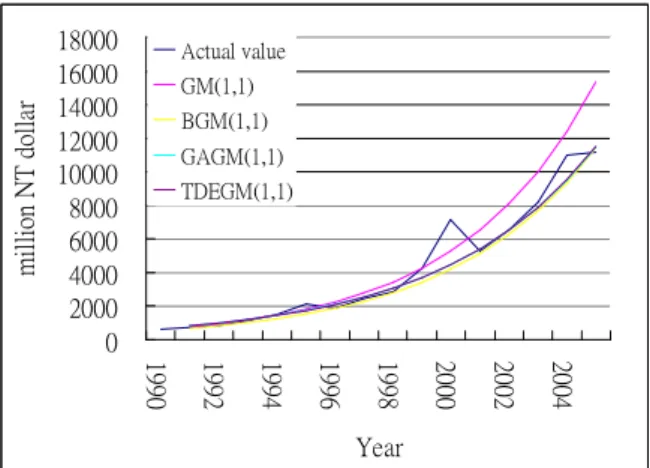
3.6. Forecasting error analysis

The predicted results obtained by the GM(1,1) model, BGM(1,1) model, GAGM(1,1), and TDEGM(1,1) model are shown in Table 1 and Figure 1. The mean absolute percentage error (MAPE) of the GM(1,1) model, the BGM, the GAGM and the TDEGM(1,1) model from 2002 to 2005 are 24.155%, 6.939%, 5.099% and 5.075%, respectively. According to the results shown above, our improved grey model TDEGM(1,1) seems to obtain the lowest post-forecasting errors of the grey models.

4. Conclusions

When the number of observations is not large, the original GM(1,1) model is powerful forecasting model. In this study, a means of accurately predicting the output value of the IC industry has been proposed by the TDEGM(1,1). The TDEGM(1,1) has a significant improvement in forecasting error. Our proposed TDEGM(1,1) is an appropriate forecasting method to yield more accurate results than the original GM(1,1) model , BGM(1,1) and GAGM(1,1).

5. References

[1] J.L. Deng “Control problems of grey systems”,

Systems and Control Letters5., pp. 288-294,

1982.

[2] C.H. Wang and L.C. Hsu “Using genetic algorithms grey theory to forecasting high technology industrial output”, Technological

Forecasting & Social Change., Vol. 195 , pp.

256-263, 2008.

[3] Ho WH, Chou JH, Guo CY (2010). Parameter identification of chaotic systems using improved differential evolution algorithm. Nonl. Dynam. 61(1): 29-41. 0 2000 4000 6000 8000 10000 12000 14000 16000 18000 19 90 1992 1994 1996 1998 2000 2002 2004 Year m il li on N T d ol la r Actual value GM(1,1) BGM(1,1) GAGM(1,1) TDEGM(1,1)

Table 1.

Forecasted values and MAPE

Year Actual

value GM(1,1) BGM(1,1) GAGM(1,1) TDEGM(1,1)

million NT

dollar

Model

value Error(%) Model

value Error(%) Model value Error(%) Model value Error(%) 1990 640 1991 724 770.957 6.486 695.205 3.977 820.494 13.328 814.789 12.540 1992 813 954.543 17.410 849.125 4.443 990.684 21.855 984.483 21.093 1993 1145 1181.846 3.218 1037.123 9.422 1196.177 4.470 1189.519 3.888 1994 1509 1463.276 3.030 1266.745 16.054 1444.294 4.288 1437.256 4.754 1995 2122 1811.722 14.622 1547.206 27.087 1743.877 17.819 1736.590 18.163 1996 1883 2243.142 19.126 1889.762 0.359 2105.601 11.822 2098.264 11.432 1997 2413 2777.295 15.097 2308.161 4.345 2542.355 5.361 2535.264 5.067 1998 2834 3438.645 21.335 2819.194 0.522 3069.703 8.317 3063.276 8.090 1999 4235 4257.481 0.531 3443.371 18.693 3706.436 12.481 3701.255 12.603 2000 7144 5271.303 26.214 4205.743 41.129 4475.243 37.357 4472.105 37.401 2001 5269 6526.544 23.867 5136.906 2.507 5403.521 2.553 5403.497 2.553 MAPE(%) (1991-2001) 13.721 11.685 12.695 12.508 2002 6529 8080.693 23.766 6274.231 3.902 6524.346 0.071 6528.868 0.002 2003 8188 10004.926 22.190 7663.364 6.407 7877.659 3.790 7888.616 3.656 2004 10990 12387.372 12.715 9360.053 14.831 9511.682 13.451 9531.556 13.271 2005 11141 15337.144 37.664 11432.395 2.616 11484.643 3.084 11516.665 3.372 MAPE(%) (2002-2005) 24.084 6.939 5.099 5.075

國科會補助計畫衍生研發成果推廣資料表

日期:2011/09/04

國科會補助計畫

計畫名稱: 不確定TS模糊模型控制系統的強健穩定及二次有限時間最佳靜態輸出回授控 制器設計研究 計畫主持人: 陳信宏 計畫編號: 99-2221-E-151-009- 學門領域: 智慧型控制

無研發成果推廣資料

99 年度專題研究計畫研究成果彙整表

計畫主持人：陳信宏 計畫編號： 99-2221-E-151-009-計畫名稱：不確定 TS 模糊模型控制系統的強健穩定及二次有限時間最佳靜態輸出回授控制器設計研究 量化 成果項目 實際已達成 數（被接受 或已發表） 預期總達成 數(含實際已 達成數) 本計畫實 際貢獻百 分比 單位 備 註 （ 質 化 說 明：如 數 個 計 畫 共 同 成 果、成 果 列 為 該 期 刊 之 封 面 故 事 ... 等） 期刊論文 0 0 100% 研究報告/技術報告 1 1 100% 研討會論文 0 1 100% 篇 論文著作 專書 0 0 100% 申請中件數 0 0 100% 專利 已獲得件數 0 0 100% 件 件數 0 0 100% 件 技術移轉 權利金 0 0 100% 千元 碩士生 2 2 100% 博士生 0 0 100% 博士後研究員 0 0 100% 國內 參與計畫人力 （本國籍） 專任助理 0 0 100% 人次 期刊論文 1 1 100% 研究報告/技術報告 0 0 100% 研討會論文 0 0 100% 篇 論文著作 專書 0 0 100% 章/本 申請中件數 0 0 100% 專利 已獲得件數 0 0 100% 件 件數 0 0 100% 件 技術移轉 權利金 0 0 100% 千元 碩士生 0 0 100% 博士生 0 0 100% 博士後研究員 0 0 100% 國外 參與計畫人力 （外國籍） 專任助理 0 0 100% 人次

其他成果

(

無法以量化表達之成 果如辦理學術活動、獲 得獎項、重要國際合 作、研究成果國際影響 力及其他協助產業技 術發展之具體效益事 項等，請以文字敘述填 列。) 無 成果項目 量化 名稱或內容性質簡述 測驗工具(含質性與量性) 0 課程/模組 0 電腦及網路系統或工具 0 教材 0 舉辦之活動/競賽 0 研討會/工作坊 0 電子報、網站 0 科 教 處 計 畫 加 填 項 目 計畫成果推廣之參與（閱聽）人數 0

國科會補助專題研究計畫成果報告自評表

請就研究內容與原計畫相符程度、達成預期目標情況、研究成果之學術或應用價

值（簡要敘述成果所代表之意義、價值、影響或進一步發展之可能性）

、是否適

合在學術期刊發表或申請專利、主要發現或其他有關價值等，作一綜合評估。

1. 請就研究內容與原計畫相符程度、達成預期目標情況作一綜合評估

■達成目標

□未達成目標（請說明，以 100 字為限）

□實驗失敗

□因故實驗中斷

□其他原因

說明：

2. 研究成果在學術期刊發表或申請專利等情形：

論文：■已發表 □未發表之文稿 □撰寫中 □無

專利：□已獲得 □申請中 ■無

技轉：□已技轉 □洽談中 ■無

其他：（以 100 字為限）

3. 請依學術成就、技術創新、社會影響等方面，評估研究成果之學術或應用價

值（簡要敘述成果所代表之意義、價值、影響或進一步發展之可能性）（以

500 字為限）

發展一新的結合正交函數計算法、田口基因演算法、矩陣測度和線性矩陣不等式技巧等有 效方法，針對非線性動態控制系統的二次有限時間最佳靜態輸出回授平行分配補償控制問 題，來設計最佳靜態輸出迴授平行分配補償控制器，並將此成果發表於國內外之期刊與會 議論文，提昇學術研究水準。