低功率MPEG-4 HE-AAC編碼器之設計

國

立

交

通

大

學

多媒體工程研究所

碩

士

論

文

低功率 MPEG-4 HE-AAC 編碼器之設計

Design of Low Power MPEG-4 HE-AAC Encoder

研 究 生：胡正倫

指導教授：劉啟民 教授

李文傑 博士

低功率 MPEG-4 HE-AAC 編碼器之設計

Design of Low Power MPEG-4 HE-AAC Encoder

研 究 生：胡正倫 Student：Cheng-Lun Hu

指導教授：劉啟民

Advisor：Dr. Chi-Min Liu

李文傑 Dr. Wen-Chieh Lee

國 立 交 通 大 學

多 媒 體 工 程 研 究 所

碩 士 論 文

A Thesis

Submitted to Institute of MultimediaEngineering College of Computer Science

National Chiao Tung University in partial Fulfillment of the Requirements

for the Degree of Master

in

Computer Science June 2007

低功率 MPEG-4 HE-AAC 編碼器之設計

中文論文摘要

器。MPEG-4 HE-AAC 編碼器包含 AAC 編碼器、SBR 編碼器和正交鏡像濾波 器組(QMF Banks)。藉由 analysis QMF bank 將輸入訊號分頻成 64 個子頻帶。低 頻訊號在經過synthesis QMF bank 還原後，交由 AAC 編碼器壓縮。而 64 個子

頻帶送往SBR 編碼器取出 SBR 參數，以供解碼器端還原高頻訊號。由於現有

的MPEG-4 HE-AAC 採用複數結構的 analysis/synthesis QMF banks，因此 QMF banks 和 SBR 編碼器都是使用複數運算。 本篇論文提出實數結構的QMF banks，無論在 QMF banks 或在 SBR 編碼 器取出SBR 參數的過程都是使用實數運算，因此計算複雜度為傳統方式的二分 之一。由於複數和實數結構的QMF banks 具有不同的物理特性，因此分析出的 64 個子頻帶也有不同的特性，造成經由實數結構 MPEG-4 HE-AAC 編碼器壓縮 出的訊號，於複數結構MPEG-4 HE-AAC 解碼器還原回的訊號會有失真。因此， 本篇論文亦提出音調性校正(Tonality Adjustment)、實化(Realification)和三種技 術，以確保降低HE-AAC 編碼器的複雜度亦維持壓縮品質。本論文亦會將低功

率技術延伸到MPEG-4 HE-AAC version 2 之上並證明其可行性。

本篇論文提出的低功率 MPEG-4 HE-AAC 編碼器架設在 NCTU HE-AAC

Encoder 之上。亦會藉由主觀及客觀測試證明低功率 HE-AAC 編碼器可維持高 品質的壓縮訊號。

Design of Low Power MPEG-4 HE-AAC Encoder

Student: Cheng-Lun Hu Advisor: Dr. Chi-Min Liu

Dr. Wen-Chieh Lee

Institute of Multimedia Engineering National ChiaoTung University

ABSTRACT

Spectral Band Replication (SBR) has been combined with MPEG-4 AAC as bandwidth extension tool. The resulting scheme is referred to as the MPEG-4 High Efficient (HE) AAC or aacPlus. With the SBR module taking care of the high frequency contents, the conventional AAC encoder can compress the low frequency part using most of the available bits. The SBR parameters are all calculated by SBR encoder in complex domain in the architecture of complex QMF. If the components in SBR encoder can be implemented in real domain, the computational complexity of HE-AAC will be reduced by half. This paper proposes the Low Power MPEG-4 HE-AAC encoder to reduce the computational complexity. The objective experiments are conducted to demonstrate the quality of Low Power HE-AAC encoder on critical music tracks. Finally, the paper will extend the Low Power technique to Parametric Stereo (PS) Encoder with HE-AAC.

致謝

Contents

Contents ...ii

Figure List... iii

Table List...v

Chapter 1 Introduction ...1

Chapter 2 Basic Component ...3

2.1 SBR Codec Overview ...3

2.2 QMF Banks in HE-AAC Encoder ...6

2.2.1 Complex QMF Banks ...7

2.2.2 Real QMF Banks...10

Chapter 3 Low Power HE-AAC Encoder...14

3.1 Basic Low Power HE-AAC Encoder...14

3.1.1 Implementation ...14

3.1.2 Complexity...18

3.1.3 Artifacts...19

3.2 Tonality Adjustment based Low Power HE-AAC encoder ...20

3.2.1 Tonality Error of Subbands in Low Power HE-AAC encoder...20

3.2.1.1 Qualitative Analysis of Tonality Error ...20

3.2.1.2 Quantitative Analysis of Tonality Error ...24

3.2.2 Implementation ...26

3.2.3 Complexity...28

3.2.4 Artifacts...29

3.3 Complexification and Realification based Low Power HE-AAC encoder....29

3.3.1 Complexification based Low Power HE-AAC encoder ...29

3.3.1.1 Complexification...29

3.3.1.2 Complexity...32

3.3.2 Realification based Low Power HE-AAC encoder ...33

3.3.2.1 Realification...33

3.3.2.2 Complexity...35

Chapter 4 Quality Assessment ...36

4.1 Experiment Environment ...36

4.2 Objective Quality Measurement in MPEG Test Tracks...37

4.3 Objective Quality Measurement in Music Database ...38

Figure List

FIGURE 1: BLOCK DIAGRAM OF HE-AAC ENCODER WITH COMPLEX QMF ...2

FIGURE 2: BLOCK DIAGRAM OF HE-AAC ENCODER WITH REAL QMF ...2

FIGURE 3: BASIC PRINCIPLE OF SBR. ...3

FIGURE 4: BLOCK DIAGRAM OF HE-AAC ENCODER. ...4

FIGURE 5: BLOCK DIAGRAM OF HE-AAC DECODER. ...6

FIGURE 6: GENERAL FRAMEWORK OF QMF BANK ...7

FIGURE 7: EXPONENTIAL MODULATED ANALYSIS QMF BANKS ...7

FIGURE 8: THE SPECTRUM OF THE ORIGINAL SIGNAL...9

FIGURE 9: COMPLEX ANALYSIS AND SYNTHESIS QMF BANK...9

FIGURE 10: THE FOUR SUBBANDS ANALYZED BY COMPLEX ANALYSIS QMF BANK ...10

FIGURE 11: THE SUBBAND Y₀(z) AFTER THE DECIMATION AND THE EXPANSION...10

FIGURE 12: THE SUBBAND Xˆ₀(z) SYNTHESIZED BY THE SYNTHESIS FILTER F₀(z)..10

FIGURE 13: REAL ANALYSIS QMF BANK ...12

FIGURE 14: THE ORIGINAL SIGNAL AND THE FOUR REAL ANALYSIS FILTERS ...12

FIGURE 15: THE FOUR SUBBANDS ANALYZED BY REAL ANALYSIS QMF BANK...12

FIGURE 16: THE SUBBANDY₁(z)AFTER THE DECIMATION AND THE EXPANSION ...12

FIGURE 17: THE SUBBANDXˆ₁(z)SYNTHESIZED BY THE SYNTHESIS FILTERF₁(z) ...13

FIGURE 18: THE SUBBANDXˆ₁(z)SYNTHESIZED BY THE SYNTHESIS FILTERF₁(z)...13

FIGURE 19: THE SUBBANDXˆ₂(z)SYNTHESIZED BY THE SYNTHESIS FILTERF₁(z) ...13

FIGURE 20: PROTOTYPE FILTER ₀( jω) e P FOR QMF BANKS IN HE-AAC ENCODER ...15

FIGURE 21: 64-BAND COMPLEX ANALYSIS FILTER BANK IN HE-AAC ENCODER...16

FIGURE 22: 64-BAND REAL ANALYSIS FILTER BANK IN HE-AAC ENCODER...16

FIGURE 23: BLOCK DIAGRAM OF TONALITY ADJUSTMENT BASED LOW POWER HE-AAC ENCODER...16

FIGURE 24: CONVENTIONAL HE-AAC ENCODING...17

FIGURE 25: BASIC LOW POWER HE-AAC ENCODING WITHOUT ENERGY ADJUSTMENT .17 FIGURE 26: HE-AAC ENCODING...18

FIGURE 28: SPECTRUM OF ORIGINAL SIGNAL...19 FIGURE 29: SPECTRUM OF CONVENTIONAL AND BASIC LOW POWER HE-AAC

ENCODER...19 FIGURE 30: WHITE NOISE SIGNAL...22 FIGURE 31: WHITE NOISE SIGNAL IN FIGURE PROCESSED BY COMPLEX-VALUE (LEFT)

/ REAL-VALUE (RIGHT) QMF BANKS (A) DECOMPOSED SUBBAND K AND K-TH ANALYSIS FILTER. (B) DOWN-SAMPLED SUBBAND K...23 FIGURE 32: TONAL SIGNAL...24 FIGURE 33: SINGLE-TONE SIGNAL IN FIGURE PROCESSED BY COMPLEX-VALUE (LEFT)

/ REAL-VALUE (RIGHT) QMF BANKS (A) DECOMPOSED SUBBAND K AND K-TH ANALYSIS FILTER. (B) DOWN-SAMPLED SUBBAND K...24 FIGURE 34: CHART OF TONALITY ERROR TE( ji, ) FOR MPEG 12...26 FIGURE 35: BLOCK DIAGRAM OF TONALITY ADJUSTMENT BASED LOW POWER

HE-AAC ENCODER...27 FIGURE 36: THE SPECTRUM OF CONVENTIONAL AND BASIC LOW POWER HE-AAC

ENCODER...28 FIGURE 37: THE SPECTRUM OF CONVENTIONAL AND TONALITY ADJUSTMENT BASED

LOW POWER HE-AAC ENCODER...28 FIGURE 38: HE-AAC ENCODER WITH COMPLEX QMF...30 FIGURE 39: FLOW CHART OF THE PROCEDURE FOR TONE DETECTION AND ALIASING

ELIMINATION...30 FIGURE 40: THE SPECTRUM OF CONVENTIONAL AND TONALITY ADJUSTMENT BASED

LOW POWER HE-AAC ENCODER...32 FIGURE 41: THE SPECTRUM OF CONVENTIONAL AND COMPLEXIFICATION BASED LOW

POWER HE-AAC ENCODER: TYPE I ...32 FIGURE 42: REALIFICATION BASED LOW POWER HE-AAC ENCODER ...34 FIGURE 43: FLOW CHART OF THE PROCEDURE OF CALCULATING SBR PARAMETERS....34 FIGURE 44: PS ENCODING WITH HE-AAC USING COMPLEX QMF BANKS ...42 FIGURE 45: PS ENCODING WITH HE-AAC USING REAL QMF BANKS...43 FIGURE 46: LOW POWER HE-AAC ENCODING WITH PS TOOL...43

Table List

TABLE 1: COMPLEXITY OF CONVENTIONAL AND BASIC LOW POWER HE-AAC

ENCODER...18 TABLE 2: TONALITY ERROR TE( ji, ) FOR MPEG 12 ...25 TABLE 3: THE AVERAGE TONALITY ERROR TE( ji, ) AND THE STANDARD DEVIATION26 TABLE 4: COMPLEXITY OF CONVENTIONAL AND LOW POWER HE-AAC ENCODER...28 TABLE 5: COMPLEXITY OF CONVENTIONAL AND LOW POWER HE-AAC ENCODER...32 TABLE 6: COMPLEXITY OF COMPLEXIFICATION BASED LOW POWER HE-AAC

ENCODER IN TERMS OF THE PERCENTAGE OF COMPLEXIFICATED SUBBANDS ...33 TABLE 7: COMPLEXITY OF CONVENTIONAL AND LOW POWER HE-AAC ENCODER...35 TABLE 8: COMPLEXITY OF COMPLEXIFICATION AND REALIFICATION BASED LOW

POWER HE-AAC ENCODER IN TERMS OF THE PERCENTAGE OF

COMPLEXIFICATED SUBBANDS...35 TABLE 9: SPECIFICATION OF MPEG 44100 CATEGORY ...37 TABLE 10: THE ODG FOR MPEG TEST TRACKS UNDER DIFFERENT KIND OF HE-AAC

ENCODERS WITH 80KBPS AND 44.1KHZ SAMPLING RATE...38 TABLE 11: THE PSPLAB AUDIO DATABASE ...39 TABLE 12: THE ODG FOR MUSIC DATABASE UNDER DIFFERENT KIND OF HE-AAC

Chapter 1

Introduction

In the conventional MPEG-4 HE-AAC encoder[1]-[4] , not only analysis/synthesis QMF (Quadrature Mirror Filter) banks, but also SBR encoder is implemented in complex domain, which results in high computational complexity. If the components can be implemented in real domain, the computational complexity of HE-AAC encoder will be reduced about 50%. This thesis focuses on the reduction of complexity in HE-AAC encoder by substituting real QMF banks for complex QMF banks. The encoder based on the approach is referred to as low power HE-AAC encoder. Low power HE-AAC encoder keeps the quality of HE-AAC encoder perceptually similar to the conventional HE-AAC encoder with a complexity improvement around two times.

In the conventional HE-AAC encoder illustrated in Figure 1, the input PCM signal is divided into 64 subbands by complex-value analysis QMF bank. The signal, synthesized from the lower 32 bands by complex-value synthesis QMF bank, is fed to the AAC encoder for waveform coding, and the higher 32 bands are fed to SBR encoder to extract side information. The above-mentioned components are all implemented in complex domain. This thesis proposes low power HE-AAC encoder to reduce the complexity of conventional one by substituting real QMF for complex QMF illustrated in Figure 2.

The thesis is organized as follows. Chapter 2 provides an overview of SBR codec and real/complex QMF banks. Chapter 3 describes details of low power HE-AAC encoder and the proposed methods used to avoid artifacts. Chapter 4 conducts the objective experiments to demonstrate the quality of low power HE-AAC encoder on critical music tracks. Chapter 5 summarizes the contribution of low power MPEG-4 HE-AAC encoder.

Figure 1: Block diagram of HE-AAC encoder with complex QMF

Chapter 2

Basic Component

This chapter presents a brief overview of SBR codec and a closer look into exponential modulated and cosine modulated QMF banks in HE-AAC encoder.

2.1 SBR Codec Overview

SBR (Spectral Band Replication) is a bandwidth extension tool integrated in AAC general audio codec. The improvement of performance is achieved by replicating the high frequency spectrum from low frequency spectrum. The replication procedure in the decoder is guided by a few amount of side information extracted from the encoder. The data rate of side information can be less than that required in conventional AAC for coding the high frequency part. The basic principle of SBR is depicted in Figure 3.

(a) Original signal (b) Reconstructed LF

(c) Replicating LF to HF (d) Reconstructed signal Figure 3: Basic principle of SBR.

In HE-AAC codec, the low frequency part shown in (b) of Figure 3 is compressed and decompressed by a waveform codec (e.g. AAC codec). Additionally, the high frequency part in the decoder is reconstructed by the replication of the low frequency spectrum shown in (c) of Figure 3, and a proper spectrum shaping which

HE-AAC Encoder

In HE-AAC encoder, the required side information which presents a parametric of high frequency part is calculated by SBR encoder in order to reconstruct the original wide-band signal. The HE-AAC encoder can be divided into the modules illustrated in Figure 4.

First, the time domain signal is fed to the 64-band analysis QMF bank. And the 64 subbands are sent to SBR encoder. In parallel, the 32 low frequency subbands are reconstructed to the time domain signal by the 32-band synthesis QMF bank in order to sent it to AAC encoder.

All of the estimation in SBR encoder is performed on QMF domain. The envelope extractor gives the time-frequency grid information and the average energy scale for each grid. The tonality estimator estimates the tonality value of 64 subbands for compensating the tone signal in SBR decoder. The inverse filter decides the inverse filtering mode which controls the high frequency whitening process. The parameter extractor delivers the control parameter to control the high frequency adjustment process.

HE-AAC Decoder

In the decoder, the received bitstream is divided into the AAC bitstream and the SBR side information. The lower frequency band component is reconstructed by the replication of low frequency subbands from AAC decoder and filtered by a 32-band QMF analyzer to provide subband signal in the QMF domain for the SBR decoder. The SBR decoding process can be considered as replication and HF adjustment. The replication process generates high frequency component by patching consecutive QMF subbands from low frequency. The block diagram of the HE-AAC decoder is shown in Figure 5. A closer look into the high frequency adjustment process is presented in the next section.

The mechanism of high frequency adjustment is to ensure that the reconstructed results perceptually be as similar as possible through the proper spectrum shaping and additional tone/noise compensation. The whole HF adjustment process can be divided into three stages, HF generation, energy scaling and tone/noise compensation.

The HF generator generates high frequency signal by replicating the low band to high band and inverse filtered by a second order complex-value predictor. The output of HF generator is referred to as high frequency generation.

After the generation stage, the envelope adjuster applies proper energy scaling on HF generation. This stage is referred to as scaling stage and the output of envelope adjuster is referred to as HF coordination.

The last stage of HF adjustment is referred to as compensation stage, which the tone/noise compensator adds tonal or noise compensation to the HF subbands. The output of tone/noise compensator is referred to as HF reconstruction.

Figure 5: Block diagram of HE-AAC decoder.

2.2 QMF Banks in HE-AAC Encoder

In HE-AAC decoder, high frequency subbands are replicated from low frequency subbands. If the real analysis QMF banks produce aliasing terms in low frequency subbands, the aliasing terms in replicated subbands can not be eliminated.

Therefore, the decoder must apply complex analysis/synthesis QMF banks rather than real analysis/synthesis QMF banks to keep replicated subbands from aliasing terms. And the HE-AAC encoder also has to use complex analysis/synthesis QMF banks to get the accurate SBR parameters corresponding to the SBR decoder.

The difference between complex and real QMF banks is introduced in 2.2.1 and 2.2.2.

2.2.1 Complex QMF Banks

Figure 6: General framework of QMF bank

The general framework of QMF bank is illustrated in Figure 6 includes four stages, analysis filter bank Hk(z) , decimators, expanders and synthesis filter bankFk(z) [5].

Figure 7: Exponential modulated analysis QMF banks

In the first stage, the original signal X(z) is split into M subbandsXk(z)by

analysis filter bankHk(z). The complex analysis QMF bank is derived from a prototype filter P₀(z). By exponential modulation, we can get the complex analysis QMF bank shown as (1) to analyze the positive frequency spectrum of the input

signal. 1 0 , ) ( ) ( ( 0.5) 2 0 ≤ ≤ − = + M k zW P z Hk Mk and k M j k M e W π − = 2 (1)

The input signal X(z) would be split into subbandXk(z) by the exponential modulated QMF bank Hk(z) as (2) ) ( ) ( ) (z X z H z X_k = _k (2)

In the second stage, the subbandsXk(z) are decimated by M toDk(z)in order

to decrease the complexity in SBR encoder/decoder by reducing the sampling rate of subbands as (3).

∑

∑

In the third stage, Vk(z)are expanded by M to Yk(z) in order to reconstruct

the original signal as (4). And we can find aliasing terms Ak(z) in )Yk(z as (5).

) ( ) ( ) ( 1 ) ( ) ( 1 ) ( ) ( 1 ) ( ) ( 1 1 z A z H z X M zW H zW X M z H z X M z V z Y k k M l l M k l M k M k k + = + = =

∑

∑

In the last stage, the aliasing terms Ak(z) have to be eliminated by the exponential modulated synthesis QMF bank in order to reconstruct the original signal without aliasing terms as (6).

) ( ) ( ) ( ) ( 1 ) ( ) ( ) ( 1 ) ( ) ( ) ( 1 ) ( ) ( ) ( ' 1 1 ^ z A z F z H z X M z F zW H zW X M z F z H z X M z F z Y z X k k k M l k l M k l M k k k k k + = + = =

∑

∑

According to (6), we know the aliasing terms '( )

z

A_k can be eliminated as long

as )H_k(z)=F_k(z . Finally, the reconstructed signal ( ) ^

z

X is combined by the

reconstructed subbands X^ k(z).

To take an example of 4-channel complex QMF bank, the original signal shown in Figure 8 is separated into four subbands by the complex QMF as shown in Figure 9 and Figure 10 in which the individual subbands are listed. Furthermore, after the decimation and the expansion, there are one original and three image components in each subband as illustrated in Figure 11. Because of the absence of negative frequency, the original component does not overlap the images. Therefore in Figure 12, by the synthesis filter F₀(z), the original component can be preserved and images can be eliminated. Similarly, the other three subbands can be obtained by the appropriate synthesis filter. By summing up the four reconstructed subbands and taking the real parts of the resultant signal, the original signal can be reconstructed without the suffering of the aliasing terms.

Figure 8: The spectrum of the original signal

Figure 10: The four subbands analyzed by complex analysis QMF bank

Figure 11: The subband Y₀(z) after the decimation and the expansion

Figure 12: The subband Xˆ₀(z) synthesized by the synthesis filter F₀(z)

2.2.2 Real QMF Banks

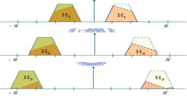
The real analysis and synthesis filter banks include both the positive and negative parts shown in Figure 13.

The framework of real QMF banks also includes four stages, analysis filter bankHk(z), decimators, expanders and synthesis filter bank Fk(z) like complex

QMF banks. But the real analysis QMF bank Hk(z) and real synthesis QMF bank )

(z

M k z V a z U a z H_k( )= _{k k}( )+ _k* _k( ) , 0≤ < (7) M k z V b z U b z F_k( )= _{k k}( )+ _k* _k( ) , 0≤ < (8) k M j k M e W π − = 2 , ( ) 0( 2( 0.5)) + = k M k k z c P zW U , ( )= * ₀( ₂−(k+0.5)) M k k z c P zW V (9) ) ( ) ( ) ( ( 0.5) 2 0 * * ) 5 . 0 ( 2 0 + + − + = k M k k k M k k k z a c P zW a c P zW H (10) ) ( ) ( ) ( ( 0.5) 2 0 * * ) 5 . 0 ( 2 0 + + − + = k M k k k M k k k z b c P zW b c P zW F (11)

To take an example of 4-channel real QMF banks, the original signal in Figure 8 is separated into four subbands by a real 4-channel analysis QMF bank shown in Figure 13. Figure 14 shows the four individual subbands.

After the decimation and the expansion, the original component of negative frequency is overlapped by the two image components produced by the original component of positive frequency shown in Figure 16, and the original component of positive frequency is overlapped by the two image components produced by the original component of negative frequency.

Therefore, by the synthesis filterF₁(z)shown in Figure 17, the synthesized

subbandXˆ₁(z)includes not only the original components but also the overlapping aliasing terms introduced from the four adjacent image bands.

By summing up the four synthesized subbands, the aliasing term will be cancelled mutually and the original signal without the aliasing terms can be reconstructed.

The aliasing term N1L of Figure 18 can be cancelled out by the aliasing term

N2R of Figure 19, and the aliasing term P1R of Figure 18 can be cancelled out by the

Figure 13: Real analysis QMF bank

Figure 14: The original signal and the four real analysis filters

Figure 15: The four subbands analyzed by real analysis QMF bank

Figure 17: The subbandXˆ₁(z)synthesized by the synthesis filterF₁(z)

Figure 18: The subbandXˆ₁(z)synthesized by the synthesis filterF₁(z)

Figure 19: The subbandXˆ₂(z)synthesized by the synthesis filterF₁(z)

Therefore, we can get the reconstructed signal in real QMF banks without aliasing terms like complex QMF banks.

However, the SBR encoder calculates the SBR parameters in the QMF domain and the subbands in real QMF domain have aliasing terms. Therefore, the SBR parameters under real QMF banks are not the same as those under complex QMF banks. In Chapter 3, the critical problem will be resolved by proposed mechanisms in low power HE-AAC encoder.

Chapter 3

Low Power HE-AAC Encoder

Through the sections from 3.1 to 3.3, three architectures are proposed to implement the low power HE-AAC encoder. In addition to specifying the low power HE-AAC encoding approaches, the performance is evaluated based upon the complexity and the quality.

In section 3.1, the basic low power HE-AAC encoder is introduced without additional mechanism to avoid artifacts. In section 3.2, Tonality Adjustment based low power HE-AAC is proposed to improve the encoding quality and keep the complexity as low as conventional HE-AAC by compensating the tonality measurement error. In section 3.3, Complexification based low power HE-AAC encoder is proposed to calculated the accurate tonality rather than just the compensated value in 3.2.

3.1 Basic Low Power HE-AAC Encoder

The complex and real-value QMF banks have been illustrated in Chapter 2. Now the real-value QMF banks are included in HE-AAC encoder.

In 3.1.1, the implement of basic low power HE-AAC encoder is specified based upon real-value QMF banks. In 3.1.2, the complexity is evaluated to prove the low power HE-AAC encoder is faster than conventional one. In 3.1.3, the artifacts spectrum of basic low power HE-AAC encoder is proposed due to the subbands’ tonality error caused by aliasing terms.

-1 -0.8 -0.6 -0.4 -0.2 0 0.2 0.4 0.6 0.8 -180 -160 -140 -120 -100 -80 -60 -40 -20 0 20

Normalized Frequency (×π rad/sample)

M ag ni tud e ( dB ) Magnitude Response in dB

Figure 20: Prototype Filter ₀( jω)

e

P for QMF Banks in HE-AAC Encoder

) (

0 ω

j e

P is a linear-phase FIR filter of length N=640 shown in Figure 20. In

conventional HE-AAC encoder, the exponential modulated analysis and synthesis QMF banks are implemented by the prototype filter ₀( jω)

e P as (12) and (13). ⎭ ⎬ ⎫ ⎩ ⎨ ⎧ _{+ − −} = ) 2 2 )( 1 2 ( 2 exp ) ( ) ( ₀ k n N M M i n p n h_k π (12) ⎭ ⎬ ⎫ ⎩ ⎨ ⎧ _{+ − +} = ) 2 2 )( 1 2 ( 2 exp ) ( ) ( ₀ k n N M M i n p n f_k π (13)

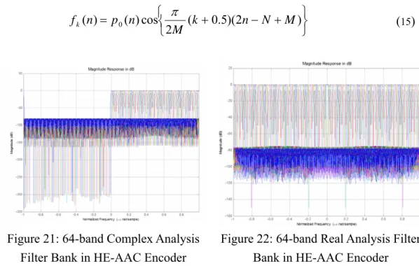
In low power HE-AAC encoder, the cosine modulated analysis and synthesis QMF banks are implemented by the prototype filter ₀( jω)

e P as (14) and (15). ⎭ ⎬ ⎫ ⎩ ⎨ ⎧ _{+ − −} = ( 0.5)(2 ) 2 cos ) ( ) ( ₀ k n N M M n p n h_k π (14)

⎭ ⎬ ⎫ ⎩ ⎨ ⎧ _{+ − +} = ( 0.5)(2 ) 2 cos ) ( ) ( ₀ k n N M M n p n f_k π (15)

Figure 21: 64-band Complex Analysis Filter Bank in HE-AAC Encoder

Figure 22: 64-band Real Analysis Filter Bank in HE-AAC Encoder

Then the real-value QMF banks are integrated in HE-AAC encoder to replace the complex-value QMF banks as Figure 23.

Figure 23: Block diagram of Tonality Adjustment based Low Power HE-AAC encoder.

Figure 24: Conventional HE-AAC Encoding

Figure 25: Basic low power HE-AAC encoding without Energy Adjustment Figure 24 and Figure 25 illustrate that there is energy difference about 3dB in HF bands encoded by conventional and basic low power HE-AAC encoder respectively. Therefore, the subbands transmitting to the SBR encoder have to be calibrated to the correct energy by 2, that is

2 ) ( ) ( ' V z z V k k = (16)

As illustrated in Figure 26 and Figure 27, the calibrated envelope based on real-value QMF banks is very close to the one based on complex-value QMF banks.

Figure 26: HE-AAC encoding

Figure 27: Low Power HE-AAC encoding with Energy Adjustment

3.1.2 Complexity

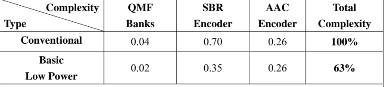
The conventional type of HE-AAC encoder means HE-AAC encoder with complex-value QMF banks. The total complexity is assumed as 100 percent. The complexity of QMF banks, SBR encoder and AAC encoder are 4, 70 and 26 percent according to the computational amount in Table 1.

Due to the half encoding complexity of QMF banks and SBR encoder, the total complexity of low power one can be derived to 63 percent compared with conventional one shown in Table 1.

Complexity Type QMF Banks SBR Encoder AAC Encoder Total Complexity Conventional _{0.04 0.70 0.26 100%} Basic Low Power 0.02 0.35 0.26 63%

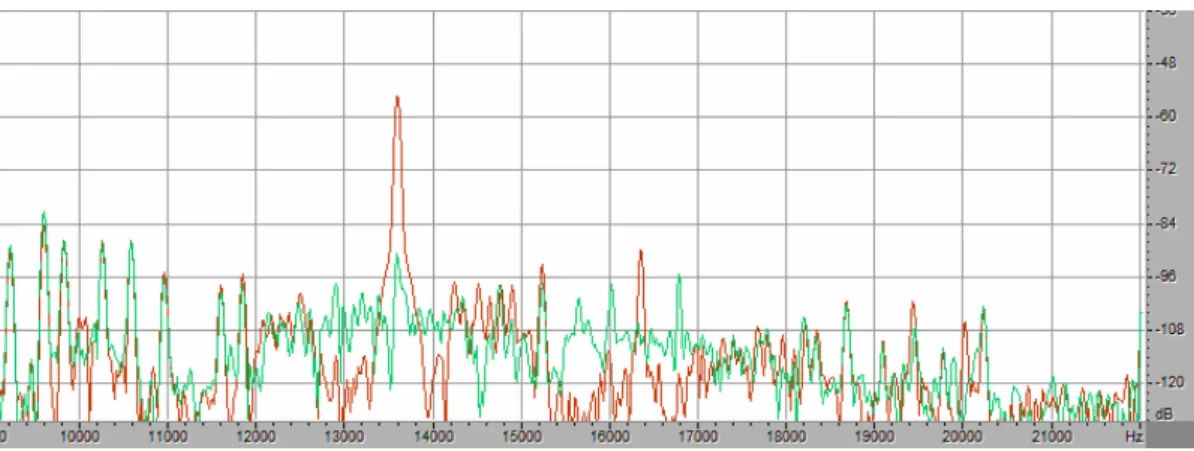
3.1.3 Artifacts

The two typical artifacts, noise overflow and tonal spike are discussed in [6] due to improper tonality measurement. The human hearing is very sensitive to such artifacts. While tonal energy is overestimated and the noise floor energy is underestimated, it will cause tonal spike.

In Figure 29, the reconstructed HF bands with real QMF banks has the noise overflow artifact in 13600 Hz and 16300 Hz because the HF subbands mixed by aliasing terms results in improper tonality measurement in SBR encoding process.

In 3.2, the tonality error of subbands is analyzed by qualitative and quantitative analysis in order to compensate the tonality error by advanced low power HE-AAC.

Figure 28: Spectrum of original signal

3.2 Tonality Adjustment based Low Power HE-AAC

encoder

In 3.2.1, the tonality measurement error can be demonstrated from qualitative and quantitative analysis. In 3.2.2, Tonality Adjustment based low power HE-AAC is proposed to compensate the tonality measurement error in order to improve the encoding quality by the result in 3.2.2. Finally, the performance is evaluated based upon the complexity and the quality.

3.2.1 Tonality Error of Subbands in Low Power HE-AAC encoder

3.2.1.1 Qualitative Analysis of Tonality Error

The section explains why the tonality of subband will be changed after substituting complex QMF banks for real QMF banks. In the beginning, some symbols are defined for the following demonstration.

] , [ ik

TC means the tonality of subband k and frame i calculated by the tonality

estimator in conventional HE-AAC encoder. The tonality error under complex-value QMF banks can be defined as (17).

63 0 , ] , [ ] , [ ] , [ ] , [ = − ≤k≤ t k E t k EN t k E t k TC (17) ] , [ tk

T_R means the tonality of subband k and frame i calculated by the tonality estimator in low power HE-AAC encoder. The tonality error under real-value QMF banks can be defined as (18).

63 0 , ] , [ ] , [ ] , [ ] , [ _' ' ' ≤ ≤ − = k t k E t k EN t k E t k TR (18) ] , [ tk

E means the energy of the k-th subband in t-th frame. and EN [ tk, ] means the noise energy of the k-th subband in i-th frame.

The tonality error can be defined as (19) in order to know the degree of tonality measurement error. 63 0 , ] , [ ] , [ ] , [ = − ≤ ≤ − k t T k t T k t k TR C R C (19)

The following examples illustrate that the tonality error is getting serious with the decrease of TR will be explained in this section. It illustrates the reason why

R

T is lower than T in noise-like signal and C TR is similar to T in tonal signal. C

The white noise signal shown in Figure 30 is decomposed by k-th analysis filter designed in section 3.1 to obtain the subband k in Figure 31 (a). Then the subband k is down-sampled in Figure 31 (b).

Because the tonality estimator calculates the tonality of down-sampled signal, the difference of the down-sampled subband spectrum between complex-value QMF banks in Figure 31 (b.1) and real-value QMF banks in Figure 31 (b.2), can be analyzed to explain why TR is lower than T in noise-like signal. C

In conventional HE-AAC encoder using complex-value QMF banks, there is no negative frequency signal produced by complex-value analysis filter in the spectrum. After down-sampling by M (M=64), the down-sampled subband in Figure 31 (b.1) is located only in positive or negative frequency of spectrum.

In low power HE-AAC encoder using real-value QMF banks, originally the positive and negative frequency components of subband in Figure 31 (a.1) don’t overlap with each other. However, the two components overlap at 0, -π and π after down-sampling by M (M=64) because the bandwidth of the prototype filter is more than

M

π

.

R

T is lower than T in noise-like signal C

In Figure 31 (b.1) and (b.2), obviously the subband under real-value QMF banks is recognized as a pure white noise signal by the tonality estimator. On the

Therefore, the tonality of subband under complex-value QMF banks is higher than which is processed under real-value QMF banks.

-1 -0.8 -0.6 -0.4 -0.2 0 0.2 0.4 0.6 0.8 -20 -10 0 10 20 30 40 50

Normalized Frequency (×π rad/sample)

M ag ni tud e ( dB ) Magnitude Response in dB

Figure 30: White noise signal

-1 -0.8 -0.6 -0.4 -0.2 0 0.2 0.4 0.6 0.8 -350 -300 -250 -200 -150 -100 -50 0 50

Normalized Frequency (×π rad/sample)

M agn itu de ( dB ) Magnitude Response in dB -1 -0.8 -0.6 -0.4 -0.2 0 0.2 0.4 0.6 0.8 -120 -100 -80 -60 -40 -20 0 20 40

Normalized Frequency (×π rad/sample)

M agn itu de ( dB ) Magnitude Response in dB (a.1) (a.2)

-1 -0.8 -0.6 -0.4 -0.2 0 0.2 0.4 0.6 0.8 -50 -40 -30 -20 -10 0 10 20 30

Normalized Frequency (×π rad/sample)

M a gni tu de ( dB ) Magnitude Response in dB -1 -0.8 -0.6 -0.4 -0.2 0 0.2 0.4 0.6 0.8 -20 -15 -10 -5 0 5 10 15 20 25 30

Normalized Frequency (×π rad/sample)

M a gni tu de ( dB ) Magnitude Response in dB (b.1) (b.2) Figure 31: White noise signal processed by complex-value (left) / real-value

(right) QMF banks (a) decomposed subband k and k-th analysis filter. (b)

down-sampled subband k

R

T is similar to T in tonal signal C

According to Figure 33 (b.1) and (b.2), obviously the signals in -0.5π and +0.5π under real-value QMF banks are recognized as tones. Under complex-value QMF banks, just the signal in -0.5π is recognized as a tone. But the noise energy under real-value QMF banks is also two times of which under complex-value QMF banks. Therefore, the tonality of subband under complex-value QMF banks is similar to which is processed under real-value QMF banks.

-80 -60 -40 -20 0 20 40 M agn itud e ( dB ) Magnitude Response in dB

Figure 32: Tonal signal -1 -0.8 -0.6 -0.4 -0.2 0 0.2 0.4 0.6 0.8 -350 -300 -250 -200 -150 -100 -50 0 50

Normalized Frequency (×π rad/sample)

Magni tude ( dB ) Magnitude Response in dB -1 -0.8 -0.6 -0.4 -0.2 0 0.2 0.4 0.6 0.8 -120 -100 -80 -60 -40 -20 0 20 40

Normalized Frequency (×π rad/sample)

Ma g n itu d e ( d B ) Magnitude Response in dB (a.1) (a.2) -1 -0.8 -0.6 -0.4 -0.2 0 0.2 0.4 0.6 0.8 -50 -40 -30 -20 -10 0 10 20 30 40

Normalized Frequency (×π rad/sample)

M agn itu de ( dB ) Magnitude Response in dB -1 -0.8 -0.6 -0.4 -0.2 0 0.2 0.4 0.6 0.8 -30 -20 -10 0 10 20 30 40

Normalized Frequency (×π rad/sample)

M agn itu de ( dB ) Magnitude Response in dB (b.1) (b.2) Figure 33: Single-tone signal processed by complex-value (left) / real-value

(right) QMF banks (a) decomposed subband k and k-th analysis filter. (b)

down-sampled subband k.

Therefore, the examples can illustrate that TR is lower than T in noise-like C

signal and TR is similar to T in tonal signal. Furthermore, The phenomenon can C

shown by quantitative analysis.

3.2.1.2 Quantitative Analysis of Tonality Error

By quantitative analysis, the tonality error between complex-value and real-value QMF banks encoder can be derived by MLD algorithm [6] in tonality estimator module of SBR encoder. And there is a trend that the tonality error is getting increasingly serious with the decrease of the tonality under real-value QMF banks.

The improper tonality measurement will result in serious artifacts in the reconstructed HF subbands. In SBR encoder, the tonality estimator applies linear prediction based MLD algorithm to calculate the tonality. In order to precisely measure the actual tonality, the poles of the linear prediction filter must match the number of tones contained in the subband, and thus the prediction order should equal to the number of tones.

In the case of missed detection, the underestimated tonal energy and the overestimated noise floor energy will result in the noise overflow in HF spectrum. Oppositely, the overestimated tonal energy and the underestimated noise floor energy will result in the tonal spike in HF spectrum.

) , ( ji

TE is the average tonality error under T_R[ tk, ] between i and j as (20).

{

}

j i

TE( , )= ( R−C[ , ])| ≤ R < ,0< < ,0≤ < (20)

Then, the average tonality error TE( ji, ) under twelve critical signal defined by MPEG can be derived as Table 2. For an example, (0,0.09) in es01 means the tonality error TE(0,0.09)=avg(TR₋C[k,t])=−0.37 in the case between

0 ] , [k i =

T_R and T_R[k,i]=0.09.

In general case, the average tonality error TE( ji, ) is getting increasingly serious with the decrease of TR shown in Figure 34 as qualitative analysis in

3.2.1.1. ) ,

( ji es01 es02 es03 sc01 sc02 sc03 si01 si02 si03 sm01 sm02 sm03 (0.90,0.99) 0.05 0.04 0.11 0.05 0.00 0.07 0.05 0.01 0.06 0.06 0.04 0.04 (0.80,0.89) 0.01 0.04 0.02 0.00 0.00 0.02 -0.02 0.01 -0.02 -0.01 -0.01 0.01 (0.70,0.79) -0.05 -0.01 -0.02 -0.07 -0.04 -0.04 -0.09 0.03 -0.10 -0.09 -0.09 -0.06 (0.60,0.69) -0.07 -0.02 -0.07 -0.10 -0.09 -0.08 -0.12 -0.01 -0.13 -0.13 -0.12 -0.10 (0.50,0.59) -0.10 -0.07 -0.06 -0.13 -0.13 -0.12 -0.15 -0.05 -0.17 -0.16 -0.15 -0.14 (0.40,0.49) -0.13 -0.09 -0.11 -0.16 -0.17 -0.16 -0.19 -0.09 -0.22 -0.19 -0.17 -0.17 (0.30,0.39) -0.17 -0.14 -0.15 -0.20 -0.21 -0.20 -0.23 -0.16 -0.28 -0.24 -0.18 -0.22 (0.20,0.29) -0.23 -0.20 -0.20 -0.23 -0.25 -0.25 -0.27 -0.21 -0.31 -0.29 -0.21 -0.26 (0.10,0.19) -0.29 -0.26 -0.26 -0.28 -0.30 -0.30 -0.32 -0.27 -0.34 -0.36 -0.27 -0.31

) ,

( ji Average Standard Deviation

(0.90,0.99) 0.0489 0.0421 (0.80,0.89) 0.0004 0.0531 (0.70,0.79) -0.0566 0.0732 (0.60,0.69) -0.0942 0.0950 (0.50,0.59) -0.1254 0.1210 (0.40,0.49) -0.1622 0.1411 (0.30,0.39) -0.2062 0.1549 (0.20,0.29) -0.2475 0.1690 (0.10,0.19) -0.3006 0.1748 (0.00,0.09) -0.3798 0.1720

Table 3: The average tonality error TE( ji, ) derived from Table 2 and the standard deviation -0.5 -0.4 -0.3 -0.2 -0.1 0 0.1 0.2 0.90~0.99 0.80~0.89 0.70~0.79 0.60~0.69 0.50~0.59 0.40~0.49 0.30~0.39 0.20~0.29 0.10~0.19 0~0.9 Real Tonality T on ality E rr or es01 es02 es03 sc01 sc02 sc03 si01 si02 si03 sm01 sm02 sm03

Figure 34: Chart of tonality error TE( ji, ) for MPEG 12

In 3.2.2, the influence of aliasing effect on low power HE-AAC encoding quality is introduced. And the tonality adjustment based approach is proposed to eliminate aliasing effect in low power HE-AAC encoder.

3.2.2 Implementation

The tonality adjustment based HE-AAC encoder compensates the tonality error to the 64 subbands T_R( tk, ) according to the compensation function CF(T_R(k,t)) designed by the quantitative analysis result in 3.2.1.2. And the compensated tonality

) , ( ' t k TR is defined as (21).

)) , ( ( ) , ( ) , ( ' t k T CF t k T t k T_R = _R + _R (21)

Compensation function CF(T_R(k,t)) is defined as (22) according to the result of

Table 3.

⎣

⎦

The tonality adjustment based HE-AAC encoder can be designed as Figure 35.

Figure 35: Block diagram of Tonality Adjustment based Low Power HE-AAC encoder.

Compared with the spectrum of basic low power HE-AAC encoder in Figure 36, the tone located in 16300 Hz of Figure 37 is compensated perfectly. And the tone located in 13600 Hz in Figure 37 is compensated better than the tone in Figure 36.

Figure 36: The spectrum of conventional and basic low power HE-AAC encoder

Figure 37: The spectrum of conventional and tonality adjustment based low power HE-AAC encoder

3.2.3 Complexity

Due to the half encoding complexity of QMF banks and SBR encoder and no additional complexity in the procedure of tonality adjustment, the total complexity of Tonality Adjustment based low power HE-AAC encoder can be derived to 63 percent compared with conventional one shown in Table 4.

Complexity Type QMF Banks SBR Encoder AAC Encoder Total Complexity Conventional _{0.04 0.70 0.26 100%} Tonality Adjustment Low Power 0.02 0.35 0.26 63%

3.2.4 Artifacts

Figure 37 clearly displays that the tonal spike artifact in 16300 Hz is eliminated due to the tonality compensation. But the noise overflow artifact in 13600 Hz still can not be eliminated completely. In 3.3, Complexification and Realification based low power HE-AAC encoder is proposed to avoid the aliasing effect for subbands’ tonality more efficiently.

3.3 Complexification and Realification based Low Power

HE-AAC encoder

3.3.1 Complexification based Low Power HE-AAC encoder

As mentioned above, both real and complex QMF have the aliasing-free property. Compared with complex-value QMF, real-value QMF banks have to eliminate the aliasing terms by the mutual cancellation due to the presence of negative frequency. Therefore, Complexification is proposed to avoid the quality degradation in HF subbands by means of eliminating the aliasing terms within subbands.

3.3.1.1 Complexification

Figure 38 illustrates the architecture of complexification based low power HE-AAC encoder integrated with the tonality adjustment introduced in 3.2. Figure 39 shows the procedure of tonality adjustment and complexification.

Figure 38: HE-AAC encoder with complex QMF

According to the statistics about tonality error in Table 3, the complexification should be opened while the subband has a high tonality error TE[ ik, ] in order to avoid the aliasing effect by eliminating aliasing terms within the subband. Besides, the subband which does not have a high tonality error would be adjusted the tonality according to the approach in 3.2.

The impulse responses of exponential/cosine modulated analysis/synthesis QMF banks hk(n)and )fk(n are introduced in 3.1. And the equation (12)-(15)

demonstrate the difference between the real QMF and complex QMF is on the imaginary part as (23) and (24).

)} 2 )( 5 . 0 ( 2 sin{ ) ( 0 k n N M M n p π + − − , (23) )} 2 )( 5 . 0 ( 2 sin{ ) ( 0 k n N M M n p π + − + . (24)

Complexification activates the computation of the imaginary part to remove the aliasing in high tonality error subbands.

Furthermore, the real-based correlation data for Levinson-Durbin algorithm[7] calculated by the tonality estimator can be used in the complex-based correlation data for complex-based tonality estimation. Hence, tonality estimator does not result in extra complexity because the related data can be reused to estimate the complex tonality TC[ ik, ].

Figure 41 illustrates the quality improvement of the subband and demonstrates that the tonality measurement error can be avoided by complexification mechanism better than Tonality Adjustment based low power HE-AAC encoder.

Figure 40: The spectrum of conventional and Tonality Adjustment based low power HE-AAC encoder

Figure 41: The spectrum of conventional and Complexification based low power HE-AAC encoder: Type I

3.3.1.2 Complexity

In Table 5, it shows that the percentage of complexificated subband can not be more than 41.5%. That means the amount of complexificated subbands can not be more than 26 for every frame.

The major reason for the huge total complexity in Complexification based encoder is that the procedure to complexificate subbands does not have efficient fast algorithm. Therefore, Realification based low power HE-AAC encoder is proposed in the next section 3.3.2. It has the same encoding quality like Complexification based one, but it has much lower encoding complexity.

Complexity Type QMF Banks SBR Encoder AAC Encoder Total Complexity Conventional _{0.04 0.70 0.26 100%} Complexification 0.027+0.53x 0.35+0.35x 0.26 (63.7+88x)%

Table 5: Complexity of conventional and low power HE-AAC encoder x: Percentage of complexificated subbands

x Total Complexity 0% 63.7% 10% 72.5% 20% 81.3% 30% 98.9% 41.5% 100% Table 6: Complexity of Complexification based low power HE-AAC encoder in

terms of the percentage of complexificated subbands

3.3.2 Realification based Low Power HE-AAC encoder

3.3.2.1 Realification

In Realification based HE-AAC encoder, it decomposes the PCM samples just by complex-value QMF banks. And it reconstructs the LF signal by the real part of subbands through real-value synthesis QMF bank.

According to the tonality T_R[ ik, ] calculated by the real part of subbands, the

tonality error can be derived from Table 3. Then the encoder will calculate the imaginary tonality by the imaginary part of subbands while subbands has high tonality error.

Therefore, the procedure of calculating SBR parameters under Realification based SBR encoder shown in Figure 42 is the same as that under Complexification based SBR encoder. And the encoding quality is completely the same as that of Complexification based one.

Figure 42: Realification based low power HE-AAC encoder

3.3.2.2 Complexity

In Table 7, it shows that the complexity of Complexification based encoder is more than that of Realification based one as long as the percentage of complexificated subband is more than 2.5%. And the encoding quality of Realification based HE-AAC encoder is as good as that of Complexification based one. Therefore, Realification based low power HE-AAC is better than Complexification based low power HE-AAC encoder in terms of complexity. And it can keep the encoding quality from degradation the same as Complexification based encoder. Complexity Type QMF Banks SBR Encoder AAC Encoder Total Complexity Conventional _{0.04 0.70 0.26 100%} Complexification 0.027+0.53x 0.35+0.35x 0.26 (63.7+88x)% Realification 0.04 0.35+0.35x 0.26 (65+35x)%

Table 7: Complexity of conventional and low power HE-AAC encoder x: Percentage of complexificated subbands

Type x

Total Complexity in Complexification based encoder

Total Complexity in Realification based encoder

0% 63.7% 65% 2.5% 65.9% 65.9% 20% 81.3% 72% 40% 98.9 79% 41.5% 100% 79.5% 60% 116.5% 86% 80% 134.1% 93% 100% 151.7% 100%

Table 8: Complexity of Complexification and Realification based low power HE-AAC encoder in terms of the percentage of complexificated subbands

Chapter 4

Quality Assessment

4.1 Experiment Environment

Computer Status

Platform Personal Computer

Operating System Windows XP

CPU AMD Turion™ 64 X2 Mobile Technology TL-56 1.8 GHz

Memory 2 GB DDR2

Headphone

Amplifier Zen Class A Headphone Amplifier

Headphone AKG K-501

Objective Quality Measurement Tool

For objective quality evaluation, the thesis mainly adopts the PEAQ system (perceptual evaluation of audio quality) [8] which is the recommendation system by ITU-R Task Group 10/4. The system includes a subtle perceptual model to measure the difference between two tracks. The objective difference grade (ODG) is the output variable from the objective measurement method. The ODG values should range from 0 to −4, where 0 corresponds to an imperceptible impairment and −4 to impairment judged as very annoying. The improvement up to 0.1 is usually perceptually audible. The PEAQ has been widely used to measure the compression technique due to the capability to detect perceptual difference sensible by human hearing systems.

4.2 Objective Quality Measurement in MPEG Test Tracks

Signal Description Track

Signal Mode Time Remark

1 es01 Vocal

(Suzan Vega) Stereo 10s (c)

2 es02 German speech Stereo 8s (c)

3 es03 English speech Stereo 7s (c)

4 sc01 Trumpet solo

and orchestra Stereo 10s (d)

5 sc02 Orchestral piece Stereo 12s (d)

6 sc03 Contemporary

pop music Stereo 11s (d)

7 si01 Harpsichord Stereo 7s (b)

8 si02 Castanets Stereo 7s (a)

9 si03 pitch pipe Stereo 27s (b)

10 sm01 Bagpipes Stereo 11s (b)

11 sm02 Glockenspiel Stereo 10s (a) (b)

12 sm03 Plucked strings Stereo 13s (a) (b) Description:

(a) Transients: pre-echo sensitive, smearing of noise in temporal domain. (b) Tonal/Harmonic structure: noise sensitive and roughness.

(c) Natural vocal (critical combination of tonal parts and attacks): distortion sensitive, smearing of attacks.

(d) Complex sound: stresses the Device Under Test.

Table 9: Specification of MPEG 44100 category

In the past few years, we have considered the design of AAC and HE-AAC encoders. The resultant AAC encoder is referred to as the NCTU HE-AAC [9]. The proposed Low Power architecture is also integrated in the NCTU HE-AAC. The objective experiments are conducted to demonstrate the quality of Low Power HE-AAC encoder on critical music tracks.For objective quality evaluation, the PEAQ system (perceptual evaluation of audio quality) which is the recommendation system by ITU-R Task Group 10/4 is adopted. The system includes a subtle perceptual model

is the output variable from the objective measurement method. The ODG values should range from 0 to −4, where 0 corresponds to an imperceptible impairment and −4 to impairment judged as very annoying. The improvement up to 0.1 is usually perceptually audible. The PEAQ has been widely used to measure the compression technique due to the capability to detect perceptual difference sensible by human hearing systems. The quality assessment of twelve test tracks recommended by MPEG are shown in Table 10.

80k (1) (2) (3) (4) es01 -0.68 -0.7 -0.69 -0.68 es02 -0.57 -0.58 -0.57 -0.56 es03 -0.8 -0.87 -0.8 -0.8 sc01 -0.98 -0.99 -0.99 -0.99 sc02 -1.21 -1.16 -1.21 -1.22 sc03 -1.13 -1.13 -1.14 -1.13 si01 -1.61 -1.6 -1.62 -1.59 si02 -1.02 -1.05 -1.08 -1.04 si03 -1.62 -1.65 -1.65 -1.62 sm01 -1.58 -1.82 -1.69 -1.63 sm02 -1.58 -1.63 -1.59 -1.57 sm03 -1.32 -1.3 -1.33 -1.32 AVG -1.175 -1.21 -1.19 -1.179

Table 10: The ODG for MPEG Test Tracks under different kind of HE-AAC encoders with 80kbps and 44.1kHz sampling rate.

(1): Conventional HE-AAC encoder (2): Basic low power HE-AAC encoder

(3): Tonality Adjustment based HE-AAC encoder

(4): Complexification\Realification based HE-AAC encoder

4.3 Objective Quality Measurement in Music Database

From previous section, the proposed methods are verified on MPEG test set. However, there are only twelve tracks in MPEG set, but the proposed methods need great quantity of test tracks to prove its possible risk and robustness. Table 11 shows the audio database. There are 15 categories and 320 test tracks in this audio database. Each category has its signal properties. With these large numbers of experiments, the

quality of proposed methods can be assessed. And Table 12 shows the quality assessment of music database under different kind of HE-AAC encoders with 80kbps and 44.1kHz sampling rate.

Bitstream Categories # of tracks Remark

1 ff123 101 Killer bitstream collection from ff123 2 Gpsycho 24 LAME quality test bitstream

3 HA64KTest 37 64 kbps test bitstream for multi-format in HA forum.

4 HA128KTestV2 12 128 kbps test bitstream for multi-format in HA forum.

5 horrible_song 16 Collections of critical songs among all bitstreams in PSPLab.

6 ingets1 5 Bitstream collection from the test of OGG Vorbis pre 1.0 listening test

7 MPEG 12 MPEG test bitstream set for 48000Hz. 8 MPEG44100 12 MPEG test bitstream set for 44100 Hz. 9 Phong 8 Test bistream collection from Phong

10 PSPLab 37 Collections of bitstream from early age of PSPLab. Some are good as killer.

11 Sjeng 3 Small bitstream collection by sjeng.

12 SQAM 16 Sound quality assessment material recordings for subjective tests

13 TestingSong14 14 Test bitstream collection from rshong, PSPLab. 14 TonalSignals 15 Artificial bitstream that contains sin wave etc. 15 VORBIS_TESTS_

Samples 8 Eight Vorbis testing samples from HA Table 11: The PSPLab audio database

80k (1) (2) (3) (4)

ff123 -1.305 -1.314 -1.306 -1.307

Gpsycho -1.205 -1.217 -1.210 -1.210

HA64KTest -1.149 -1.154 -1.158 -1.156

MPEG -1.716 -1.731 -1.718 -1.719 MPEG44100 -1.175 -1.214 -1.193 -1.179 Phong -1.131 -1.129 -1.146 -1.143 PSPLab -1.266 -1.296 -1.304 -1.304 Sjeng -0.853 -0.877 -0.812 -0.807 SQAM -1.011 -1.023 -0.998 -0.989 TestingSong14 -1.330 -1.342 -1.347 -1.333 TonalSignals -2.781 -2.875 -2.854 -2.789 VORBIS_TESTS_Samples -0.843 -0.855 -0.853 -0.845 AVG -1.277 -1.294 -1.285 -1.280

Table 12: The ODG for music database under different kind of HE-AAC encoders with 80kbps and 44.1kHz sampling rate.

(1): Conventional HE-AAC encoder (2): Basic low power HE-AAC encoder

(3): Tonality Adjustment based HE-AAC encoder

Chapter 5

Conclusion and Future Works

All the processing framework of MPEG-4 HE-AAC version-2 encoder [10][11] is based on complex-valued domain to avoid the aliasing interference from real QMF bands. Low power HE-AAC encoder [12] has reduced the computational complexity largely by adapting the real/complex QMF banks into SBR encoder with almost the same quality. This section considers the extension of the method on the PS (parametric stereo coding) encoder to design the low-power high-quality HE-AAC version-2 encoder.

The PS is a tool to compress high quality stereo audio at bit rates around 24 kbps. The PS module is used to reconstruct stereo signal from the monaural down-mixed signal according to the stereo parameters which are extracted by capturing the stereo image of the input binaural signal. The down-mix process and the stereo parameters including IID (inter-channel intensity difference), ICC (inter-channel coherence), IPD (inter-channel differences) and OPD (overall phase differences) are also based on complex QMF bands. Therefore, the computational requirement can be reduced if the complex QMF is replaced by real QMF. However, the two major issues from the introduced aliasing terms should be considered.

1. Inaccurate Parameter Estimation

Because the conventional PS decoder is based on complex-valued QMF, it assumes that all stereo parameters are extracted from the stereo complex-valued QMF in encoder part. In other word, the stereo parameters extracted from the stereo real-valued or complex/real-valued QMF will result in possible risk due to the interference of aliasing terms. For example, the aliasing terms may measure excessive or inadequate intensity levels, then cause the misestimates of IID and lead to severe artifacts such as energy overflow and noise overflow. Moreover, the huge aliasing terms in one channel may has the high correlation with the original tone component in the other channel. This leads to incorrect estimation of phase differences.

The aliasing terms will be brought into the down-mixed monaural signal. For the averaging down-mix approach, the aliasing terms can be still canceled mutually band by band due to the fixed 1/2 combination coefficient. Although the aliasing-free property can be maintained in the averaging approach, the aliasing terms will lead to the inaccurate SBR parameters for the monaural signal. Moreover, for the adaptive down-mix approach, for example the KLT (Karhunen-Loève Transform)-based method, the aliasing-free property is broken due to no-fixed combination coefficients. This means the aliasing tem will occur in the synthesized monaural signal and lead to annoying perceptual artifacts after the up-mixing process.

According to these two issues, this thesis proposes an adaptive mechanism to use real or complex QMF bands for noise-like and tonal bands to arrive the tradeoff of handling the sever aliasing suffering and reducing the time complexity. Also, the extraction method of parameters, including the stereo parameters and the optimal combination coefficient of the KLT down-mixing approach will be derived for those cases that the stereo bands are real/real and real/complex QMF bands.

The technology has been incorporated into the NCTU HE-AAC v2 encoder mentioned in AES115th-122nd convention. The objective experiments and the encoding speed evaluation are conducted to demonstrate the two dimensions of quality and speed of Low Power HE-AAC v2 encoder by comparing to the conventional HE-AAC v2 encoder.

Figure 45: PS encoding with HE-AAC using real QMF banks

Figure 46: Low Power HE-AAC encoding with PS tool

This thesis proposed the design of MPEG-4 Low Power HE-AAC encoder to reduce the computational complexity of HE-AAC encoder by four different approaches in Chapter 3. And the experiments have shown that the Low Power HE-AAC encoder keeps the quality of HE-AAC encoder perceptually similar to the conventional HE-AAC encoder. And the thesis extends the low power technique to PS encoder with HE-AAC to reduce the computational complexity.

References

[1] ISO/IEC, “Text of ISO/IEC 14496-3:2001/FPDAM 1, Bandwidth extensions,”

ISO/IEC JTC1/SC29/WG11/N5203, October 2002, Shanghai, China.

[2] M. Dietz, L. Liljeryd, K. Kjörling, O. Kunz, “Spectral Band Replication, a novel

approach in audio coding,” 112nd AES Convention, Munich, Germany, May 2002, Preprint 5553.

[3] M. Wolters, K. Kjörling, D. Homm, H. Purnhagen, “A closer look into MPEG-4

High Efficiency AAC,” 115th AES Convention, New York, USA, October 2003, Preprint 5871.

[4] H.W. Hsu, C.M. Liu, and W.C. Lee, “Audio Patch Method in MPEG-4 HE AAC

Decoder,” 117th AES Convention, San Francisco, USA, October 2004, Preprint 6221.

[5] P.P. Vaidyanathan, “Multirate Systems and Filter Banks,” Englewood Cliffs, NJ:

Prentice-Hall, 1993.

[6] H.W. Hsu, Y.C. Yang, C.M. Liu, and W.C. Lee, “Design for High Frequency

Adjustment Module in MPEG-4 HEAAC Encoder based on Linear Prediction Method,” AES 120th Convention, Paris, France, 2006 May 20 – 23

[7] N. Levinson, “The Wiener RMS (Root Mean Square) Error Criterion in Filter

Design and Prediction,” J. Math. Phys. 25, 261-278 (1947)

[8] ITU Radiocommunication Study Group 6, “Draft Revision to Recommendation

ITU-R BS.1387- Method for objective measurements of perceived audio quality.”

[9] NCTU-AAC website: http://psplab.csie.nctu.edu.tw/

[10] K.C. Lee, C.H. Yang, H.W. Hsu, W.C. Lee, C.M. Liu, and T.W. Chang, “Efficient

Design of Time-Frequency Stereo Parameter Sets for Parametric HE-AAC,” 119th AES Convention, New York, USA, October 7 – 10, 2005

[11] ITU Radiocommunication Study Group 6, “Draft Revision to Recommendation

ITU-R BS.1387- Method for objective measurements of perceived audio quality.”

[12] H.W. Hsu, C.L. Hu, C.M. Liu, W.C. Lee, “Design of Low Power MPEG-4