P E R G A M O N
computers &
mathematics
with applicationsComputers and Mathematics with Applications 40 (2000) 885-895
www.elsevier, nl/locate/camwa
T e r m i n a l - P a i r R e l i a b i l i t y
in A T M V i r t u a l P a t h N e t w o r k s
S T E E N J .Hsu,
Y u G . C H E N A N D M A R I A C . Y U A N G D e p a r t m e n t of C o m p u t e r Science and I n f o r m a t i o n E n g i n e e r i n g N a t i o n a l C h i a o T u n g University, Taiwan, R . O . C .(Received May 1998; revised and accepted March 1999)
A b s t r a c t - - T e r m i n a l - p a i r reliability (TR) in an asynchronous transfer mode (ATM) virtual path (VP) network corresponds to probabilistic quantification of robustness between two VP terminators, given the V P layout and the failure probabilities of physical links. Existing T R algorithms are shown to be unviable for ATM VP networks owing to either high complexities or failure dependency among VPs. The goal of the paper is to propose efficient algorithms for the computation of T R between
two VP terminators by means of variants of path-based and cut-based partition methods which have been effectively used for the computation of T R in traditional networks. The first variant, called the path-based virtual path reliability (PVPR) algorithm, partitions the search space based on a physical path embedding the shortest route of VPs from the source terminator to the destination terminator. The second variant, called the cut-based virtual path reliability (CVPR) algorithm, in lieu, performs
the partition on the basis of a physical cutset separating the source from the remaining terminators. In both algorithms, each subproblem is recursively processed by means of partition until the source and destination terminators are contracted or disconnected. Experimental results demonstrate that, compared to one promising T R algorithm (called EBRM), both the P V P R and C V P R algorithms improve the running time by five orders of magnitude. In particular, the C V P R outperforms EBRM more than P V P R does in terms of computation time. The two algorithms and their promising results consequently facilitate the real-time computation of the reliability or robustness of ATM VP networks.© 2000 Elsevier Science Ltd. All rights reserved.
K e y w o r d s - - A s y n c h r o n o u s transfer mode (ATM), Virtual path (VP), Terminal-pair reliability (TR), Path-based partition, Cut-based partition.
1. I N T R O D U C T I O N
Asynchronous transfer mode (ATM) [1-3] has been widely accepted to support the integration and economical t r a n s p o r t of multirate traffic in broadband integrated services digital networks (B-ISDNs) [2]. In particular, the virtual path (VP) concept [4,5] in ATM networks has been proposed to significantly reduce control costs by grouping a number of virtual channel (VC) connections into a single unit, i.e., a VP connection. In such an ATM V P network, a VC is embedded in a concatenation of one or more VPs, and a VP is embedded in a concatenation of one or more physicM links. Nodes switching and terminating VPs are called V P switches and V P terminators (or VC switches), respectively. Switches serving both functions are called V P / V C switches.
0898-1221/00/$ - see front matter (~) 2000 Elsevier Science Ltd. All rights reserved. Typeset by ~4A/tS-TEX PIh S0898-1221 (00)00204-2
The fundamental advantage of VPs is the allowance of a large group of VCs to be handled as a single unit, resulting in faster processing per connection, lower switching complexity, and superior utilization of network resources. An additional advantage is the assurance of network reliability despite link failures or network congestion by rerouting those impaired VCs in real time to alternative pre-established backup VPs [6,7]. Terminal-pair reliability (TR) in this case corresponds to probabilistic quantization of robustness of a given VP layout between any two VP terminators. As a result, the success of such real-time restoration of connections from network failures and congestion hinges on the efficiency of the TR computation. This paper aims for the design of efficient TR algorithms for ATM VP networks.
Existing TR algorithms [8-19], which have been mostly designed for traditional circuit-switch- ed-based networks, can be categorized into two classes. The first class regards link failures as independent events, whereas the second class considers failures as dependent events. In the first class [8,9,11,16-19], existing algorithms efficiently computed TR by means of the path- based [9,11] and the cut-based [8,16] partition methods. These algorithms effectively partition the search space and recursively process the generated subproblems until the source and the destination are contracted or disconnected. These algorithms are viable but inappropriate for ATM VP networks owing to failure dependency among VPs.
In the second class, the ~ model [12], requiring the specification of an exponential number of conditional probabilities of link failures, analyzed TR by chain rule expansion. The Page and Perry model [13] appliedthe pivotal decomposition theorem to factor out the dependent failures resulting in 0(2 n) of subproblems to be generated, where n is the number of links. Lam and Li [14] proposed an event-based reliability model (EBRM) to analyze TR by means of existing efficient TR algorithms of the first class with a procedure of transformation augmented. These algorithms, which incur high complexity rising exponentially with the number of links, render the TR computation for VP networks impracticable.
In this paper, we propose two efficient algorithms for the computation of TR between two VP terminators by means of variants of the path-based and cut-based partition methods. The first variant, called the path-based virtual path reliability (PVPR) algorithm, partitions the search space of the problem into a set of subproblems based on a physical path embedding the shortest route of VPs from the source terminator to the destination terminator. The second variant, called the cut-based virtual path reliability (CVPR) algorithm, instead performs the partition on the basis of a physical cutset separating the source from the remaining terminators. In both algorithms, each subproblem is recursively processed by means of partition until the source and destination terminators are contracted or disconnected.
By partitioning based on the physical links and effectively reducing the number of generated subproblems, the PVPR and CVPR algorithms, as will be shown, dramatically reduce the com- putational complexity. Experimental results demonstrate that, compared to EBRM, both the PVPR and CVPR algorithms improve the running time by five orders of magnitude. In partic- ular, the CVPR outperforms EBRM more than PVPR does in terms of computation time. The CVPR and PVPR algorithms and their promising results consequently facilitate the real-time computation of the reliability or robustness of ATM VP networks.
The rest of t h e paper is organized as follows. Section 2 presents a brief overview of the EBRM algorithm and discusses its application to ATM VP networks. The PVPR and CVPR algorithms are then formally proposed in Section 3. Experimental results are demonstrated in Section 4. Finally, Section 5 gives concluding remarks.
2. O V E R V I E W O F T H E E B R M A L G O R I T H M
The EBRM algorithm computes reliability subject to independent failure-causing events, each occurrence of which causes the simultaneous failures of several network links. Conceptually, the algorithm initially expresses the TR measurement as a function of the success/failure probabilities
of network links. This can be achieved by means of performing existing T R algorithms assuming independent network failures. Each term of the reliability function is then further expanded into a function of the occurrence probabilities of the failure-causing events. T h e algorithm is described in more detail via the following example.
Consider a network (G) with a source (s), a destination (t), and the failure-causing events, as shown in Figure 1. Based on an efficient T R algorithm [10], the T R measurement from s to t, denoted as Rel(G), can be first expressed as
Rel(G) = p i P 5 + P2P6 + p l p a p 6 + P2P4P5 - p l p 2 P s p 6 - P l P 3 P s P 6 - p l p 2 p 4 P 5 - p l p 2 p 3 p 6 - P 2 p 4 P 5 P 6 - P l P 2 p 3 P 5 P 6 + P l P 2 P 4 P 5 P 6 ,
(1)
where Pi (i = 1 to 6) represents the probability that link e~ is operational. Notice t h a t the complexity of deriving such Rel(G) in equation (1) increases exponentially with the number of network links. Since the failure-causing events are assumed to be independent, the probability t h a t a group of links are all operational is just the product of the nonoccurrence probabilities of the events involved. Consequently, Rel(G) can be further expressed as
Rel(G) = PaPbPe + P a P d p e - PaP~PdPe,
(2)
where p~, x = a, b, c, d, or e, corresponds to the probability of nonoccurrence of failure-causing event x. It is also worth noticing that, since the number of product terms in Rel(G) increases exponentially with the number of network links, the transformation from equation (1) to (2) requires exponential time.
(a) Network G.
Failure-Causing Events Pertinent Links
a e l , e 2
b ea,e4,e5
C e 3 , e 4
d e6
e el,e3,e4,e6
(b) Failure-causing events and pertinent links. Figure 1. An example for illustrating the EBRM algorithm.
By regarding VPs and physical links as network links and failure-causing events, respectively, the E B R M algorithm can be applied to the computation of T R in ATM VP networks. Unfortu- nately, as depicted in the previous example, both deriving a T R expression and transforming a VP-based T R expression to a link-based T R expression require time complexities which increase exponentially with the number of VPs [20]. Consequently, the E B R M algorithm is impractical for ATM networks which often possess a large number of VPs. To alleviate this problem, we propose two efficient T R algorithms, namely the P V P R and C V P R algorithms, by means of the path-based and the cut-based partition methods described as follows.
3. P V P R
A N D
C V P R
A L G O R I T H M S
Generally, the P V P R and C V P R algorithms employ the factoring theorem [13] to partition the search space by means of different physical partition bases. Given an ATM network (G) with a source terminator (s) and a destination terminator (t), the P V P R algorithm uses the physical path (referred to as the shortest s - t p a t h hereafter) embedding the shortest route of
VPs from s to t as the partition basis in an a t t e m p t to locally minimize the number of generated subproblems. In contrast, the C V P R algorithm employs the physical cutset (referred to as the
_ e x f V P 2 Source s ~ V P switch y
egl'l 7//'z lilt'- vP1
v e 3 ~ e 2
v P / v c switch x - I' e5 - Destination tVP4
VP 1 (embedded in {el, e2})
VP2
(embedded[ N N , ~ V P 3 (embedded in {e4, e3, e2})in {el, e3} ) ~ . ~
-- V p 4 - -
(embedded in { e5 }) (a) An ArM network with a VP layout. (b) Equivalent VP graph G.
Figure 2. An example of an ATM VP network.
s o u r c e c u t hereafter), separating s from the remaining terminators, as the partition basis to reduce the complexity of partitioning. In b o t h algorithms, each subproblem is recursively processed by means of partition until s and t are contracted or disconnected.
W i t h o u t loss of generality, we assume t h a t V P s in network G are unidirectional. T h e failures of physical links are assumed to be mutually independent. Figure 2a depicts an example of an A T M VP network, consisting of a V P / V C switch, a VP switch, and two VP terminators. Moreover, Figure 2b shows the equivalent VP graph which will be used throughout the rest of the section. Notice t h a t the equivalent VP graph is logically identical to the original ATM VP network. T h e t r a n s f o r m a t i o n between two graphs requires no c o m p u t a t i o n time and is only illustrated for easier illustration purpose.
3.1. P V P R A l g o r i t h m
Initially, let us define the length of a VP to be the number of physical links traversed by this VP. T h e s h o r t e s t s - t V P r o u t e is defined as the minimum-length route of V P s from s to t. Moreover, the s h o r t e s t s - t p a t h is defined as the set of the physical links comprising the shortest
s - t VP route. Now, by the factoring theorem, the T R measurement from s to t in G, i.e., Rel(G), can be represented given the shortest s - t p a t h {el, e 2 , . . . , et }, as
Rel(G) = ql × R e l ( G - el) + P l q 2 x R e l ( G * el - e2) + ...
+ P l . . . P t - l q l x R e l ( G * el * . . . * et_l - el) + p l . . . P t - l P t × R e l ( G * c l * - - - * et-1 * el), where p~ (q~) represents the success (failure) probability of link e~, and " . " ( " - " ) represents the contracting (deleting) operation of physical links. A VP e m a n a t i n g from s is contracted if all the physical links used by the V P are contracted, resulting in the contraction of the ending t e r m i n a t o r of the VP with s. Notice t h a t Rel(G * el * .-. * e t - t * el) is equal to one due to the contraction of s and t. Subproblems Rel(G * el * . . . * ei-1 - e~), i = 1 to l, are then recursively processed by means of partitioning based on the shortest s - t p a t h until s and t are disconnected. T h e detailed P V P R algorithm is further outlined in Figure 3.
An example of illustrating how the P V P R algorithm performs for the network given in Figure 2 is shown in Figure 4. Initially, the shortest s - t VP route {VP1} and the shortest s - t p a t h {el, e2} can be simply derived according to the existing shortest p a t h algorithms [21] and the definition given above. Rel(G) can thus be decomposed as Rel(G) = ql x Rel(G - el) + P l q 2 x
Rel(G * el - e2) + PIP2. Both subproblems ReI(G - el) and Rel(G • el - e2) are continuously processed by means of partition until s and t are disconnected. Finally, Rel(G) is expressed as Rel(G) = qlP4P3P2 + Plq2P3P5 + PIP2.
T h e P V P R algorithm successfully reduces the computational complexity by performing the partition on the basis of physical links which usually yield smaller space t h a n t h a t of VPs. Notice that, based on the P V P R algorithm, the numbers of subproblems generated by partitioning are locally minimized at the expense of executing the path-searching algorithm for finding the partition basis in each subproblem.
A l g o r i t h m Rel _PVPR(G)
I n p u t : ATM V P network G with source s, destination t, and the failure probabilities of the physical links;
O u t p u t : Terminal-pair reliability R between s and t; B e g i n
R := 0.0; factor : : 1.0; if s = t r e t u r n 1.0;
Determine the shortest
s-t
p a t h {el, e2, . . . ,el}
in G; i f {el,e2 . . . . ,e/} ~ q}for i : = 1 to l d o R : : R + factor ×
qi
x R e l _ P V P R ( G - ei);G::G *ei;
factor := factor
×Pi;
e n d f o r R := R + factor; e n d i f r e t u r n R; E n d Figure 3. T h e P V P R algorithm.Network G . / ~ VPI { el, e2 }
/" ~
VP3~e4,
e3, e2}VP2{el, e3}l
~ }\ ~
" ~ I Shortests-tVProute={VP1}
\
•
~, ~ / Shortest s - t p a t h = { e l , e2} Delete e l ~Shortest s--t VP r o u t e / / ~
~ 1
={VP3}
[~VV3{e4,
e3, e2} Shortest s-t path \ ~ ~ / ={e4, e3, e2} \ ~ 7e Q *
Contract el,~
~:~Contract
el and e2Detete e2 v
/ ~
G"*el-e2
G'el*e2
(~VP2{e3 } ~
s and t are contracted\ ~ A /
K ~ / Shortest s-t VP route={
VP2, VP4}
", v r41efll " Shortest s-tpath={e3, es}Delete e 3 ~ Contract
e3,~
Detete e5 Q ~:~Contract e3 and e5 G * e 1 "e2"e 3
s and t axe disconnected
G*el-e2*e3-e5
s and t are disconnected
G*el-e2*e3*e5
s and t are contracted Figure 4. T h e P V P R a l g o r i t h m - - a n example.
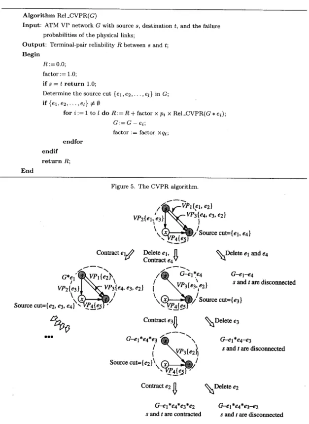
3.2.
C V P R A l g o r i t h mIn t h e C V P R algorithm, the partition is performed based on the s o u r c e c u t , defined as the set of physical links first encountered by the V P s e m a n a t i n g from s. Given the source cut {el, e 2 , . . . , el}, by the factoring theorem, Rel(G) can be represented as
Rel(G) = p l × R e I ( G * el) + q l p 2 x R e l ( G - el * e2) + . . .
+ q t . . . q t - l P t x Rel(G - e l . . . e t - 1 * e l ) + q l . . . q l - l q z x Rel(G - el . . . el-1 - ez), where pi (qi) represents the success (failure) probability of link ei and " . " ( " - " ) represents the contracting (deleting) operatio n of physical links. Similar to the P V P R algorithm, a V P e m a n a t i n g from s is contracted if all the physical links used by the V P are contracted. Notice t h a t Rel(G - et . . . el-1 - el) is equal to zero due to the disconnection between s and t.
A l g o r i t h m Rel _CVPR(G)
Input: ATM VP network G with source s, destination t, and the failure probabilities of the physical links;
O u t p u t : Terminal-pair reliability R between s and t; Begin
R:=O.O; factor :---- 1.0; if s = t r e t u r n 1.0;
Determine the source cut {el, e 2 , . . . , el} in G;
if {el,e2 . . .
et} 5 ~ 0
f o r i := 1 to l do R := R + factor x
Pi
× Rel_CVPR(G *ei);
G:=G-ei;
factor := factor
xqi;
endforendif r e t u r n R; End
Figure 5. The CVPR algorithm.
Contract e l / ~
VP2{el,le3 } ~ N ~ Ve31e4' e3' e2}
\ ~ /
\ ~ / S o u r c e cut=-{el, e41 Delete el, ~ ~ D e l e t e el and e4
Contract e4
G'~I'~PI{e2}~\
VP2 {~3 }fl~
~VP3]{e4, e3. e2}
N ¢
Source cut={e2, e3, e4} ~
/ ~ G-el*e4 G-el-e 4 ( - N N ~ 3 { e 3 : e 2 } s a n d t are d i s c o r m e c t e d \ \ ~ / / S o u r c e cut={ e3 } Contract e3~ Cr-el*e4*e~ ~ ~ ' \ ( N~.P3{e2~ I Source cut={ e2 } \ \ . ~ / / • ~ 4 t ~ " Contract e2
G-el*e4*e3*e 2
s a n d t are c o n t r a c t e d~
Delete e 3 G-el*e4-e 3 s and t a r e d i s c o n n e c t e d~
Delete e2 G--e I *e4*e3-e2 s a n d t are d i s c o n n e c t e dFigure 6. The CVPR algorithm--an example.
S u b p r o b l e m s R e l ( G - el . . . ei-1 *
ei),
i = 1 to l, are t h e n recursively processed b y m e a n s of p a r t i t i o n i n g based on t h e source cut until s a n d t are c o n t r a c t e d or disconnected. T h e detailed C V P R a l g o r i t h m is f u r t h e r outlined in F i g u r e 5.An e x a m p l e of illustrating how t h e C V P R a l g o r i t h m p e r f o r m s for t h e n e t w o r k given in F i g u r e 2 is s h o w n in F i g u r e 6. Initially, by definitions, t h e source cut is derived as {el, e4}. R e l ( G ) is t h e n d e c o m p o s e d as Rel(G) = Pl × R e l ( G • el) +
qlP4 x
R e l ( G - el * e4). B o t h s u b p r o b l e m s(I)[17]
÷
(6)[17] (2)[17] [7) [ 17] S ~ t (3) [17] (8)[17] (4)[17] s ~ t (9)[17] (5)[17] (10)[17] (11) NSFNET (12)[171 (13)[181 i(14)[17] (15)[9,13] (16)[171 (17)[17] ~ a (20)[19] L e g e n d : ( i ) [ j 1 : ( e x a m p l e index) [ B e n c h m a r k s o u r c e p a p e r ( s ) l F i g u r e 7. B e n c h m a r k s . C o m p u t a t i o n t i m e • 1o daysp 5 days iday ... P V P R / / × x C V P R / . - ~ .. /
+ - - - - - - + S & P - b a s e d E B R M / ] ~ " 1 hour * - - - - - ' D & G - b a s e d E B R M . / / / lmin ' '~ ' / " 1 4 ( / ~ " ~ - - ~ . . - 10n~ 0.1 ms J , L L ~ ~. • • • 1 2 3 4 5 6 7 8 9 10 11 12 13 14 15 16 17 18 (a) M e a n V P o u t - d e g r e e = 3.0 B e n c h m a r k C o m p u t a t i o n t i m e > 10 daysp ~ - - - ' - e - - - - P - - - - I ' - - ' - P - - q - - / ; ; ~ ~ ; ~- ; ;- " / / 5 days / / a t 1 day //
lhour / : . ~ . . . . 4 , . - . . . ~ . ¢ / # 1 . . 100 m s iotas / ~ _ . - ~ - " ~ x X C V P R 1 ~ 4 ~ - " - ' ~ ~ + - - - - - - + S & P - - b a s e d E B R M0.1 ms a" . . .
~
, ", ¢ D¢G-~as~t EBRM
1 2 3 4 5 6 7 8 9 10 11 12 13 14 15 16 17 18 Ca) M e a n V P o u t - d e g r e e = 5.0 B e n c h m a r k C o m p u t a t i o n t i m e > 10 days /o--- - ; ~. ~, ~ ~. ; ; ; ;- ~ ; ; ; ~. ~ ,7,
ida, /
/
1
lminlsech°ur / /
1oO 1o
¢ ' . . . . . .:CVPR
1 ms + - - - - - - + S & P - - b a s e d E B R M * - - - - - "--'* D & G - - b a s e d E B R M 0.1ms Jl . . . 1'0 . . . . 2 3 4 5 6 7 8 9 11 12 13 14 15 16 17 18 (c) M e a n V P o u t - d e g r e e = 10.0 B e n c h m a r k F i g u r e 8. C o m p u t a t i o n t i m e f o r t h e b e n c h m a r k s .Number of subpmblems (normalized by the results of CVPR) 1.1 13] ," X o.gK. . . , - g " g 0.8- "@'" ", ~ , - - 4 ' " 0.7 "~" 0.6 0.5 0.4 0.3 0.2 0.1 0 I I i 2 3 4 1.1 ' ~ X v * , o 11' • . , i I i ~ t J i i 5 6 7 8 9 10 11 12 (a) Mean VP out-degree = 3.0
x xCVPR • . . . • PVPR i i I ~ i 13 14 15 16 17 18 Benchmark 1 . 0 * 0.9 , 0.8 ~" 0.7 0.6 0.5 0.4 0.3 0.2 0.1 i 2 I i 3 4 ~,- i h i L J * i i 5 6 7 8 9 10 11 12 (b) Mean VP out-degree = 5.0 ,•- - -@-. -@... x x CVPR , . . . • PVPR 13 14 15 16 17 18 Benchmark 1.1 1.0 ~ ,., ,,, 0.9 ~ - . 0.8 " ,' "~ 0.7 k / 0.6 ¥ 0.5 0.4 0.3 0.2 0.1 0 , i i 2 3 4 ',IF" " ~ " ' 4 W " ~ ' ' " 41'" i i i i i i ~ i i 5 6 7 8 9 10 11 12 13 (c) Mean VP out-degree =10.0 4 k "~-- . @ . . X X CVPR • . . . • PVPR i i i L 14 15 16 17 18 Benchmark
Figure 9. Compamson of the number of subproblems between PVPR and CVPR.
R e l ( G • e l ) a n d R e l ( G - e l * e4) are c o n t i n u o u s l y p r o c e s s e d by m e a n s of p a r t i t i o n u n t i l s a n d t are c o n t r a c t e d (as in G - e l * e4 * e3 * e2) or d i s c o n n e c t e d . Finally, R e l ( G ) is e x p r e s s e d as R e l ( G ) -- P i P 2 + Plq2P3P5 + q l p 4 p 3 p 2 . C o m p a r e d t o t h e P V P R a l g o r i t h m , t h e C V P R a l g o r i t h m m a k e s no a t t e m p t t o locally m i n i m i z e t h e n u m b e r s of s u b p r o b l e m s , t h o u g h as will be shown, g r e a t l y r e d u c e s t h e c o m p u t a t i o n t i m e for t h e p a r t i t i o n i n g of each s u b p r o b l e m . 4. E X P E R I M E N T A L R E S U L T S To d e m o n s t r a t e t h e v i a b i l i t y of o u r a l g o r i t h m s , we i m p l e m e n t e d t h e E B R M , P V P R , a n d C V P R a l g o r i t h m s in t h e C l a n g u a g e a n d e x e c u t e d t h e s e a l g o r i t h m s in S u n S e r v e x S t a t i o n 5 u s i n g a c o l l e c t i o n o f physical n e t w o r k b e n c h m a r k s [9,13,17-19], as s h o w n in F i g u r e 7. F u r t h e r m o r e , for d e r i v i n g s y m b o l i c T R e x p r e s s i o n s in t h e E B R M a l g o r i t h m , we c a r r i e d o u t t w o v e r s i o n s of i m p l e m e n t a t i o n s : S & P - b a s e d [10] a n d D & G - b a s e d [11]. M o r e o v e r , V P l a y o u t s in t h e b e n c h m a r k s w e r e r a n d o m l y c o n s t r u c t e d f r o m s p a r s e t o d e n s e (by v a r y i n g t h e m e a n V P o u t - d e g r e e ) w i t h m e a n V P l e n g t h s n e a r 2.0 in b e n c h m a r k s 1-9, 3.0 in b e n c h m a r k s 10-15, a n d 4.5 in b e n c h m a r k s 16-18, a n d a s t a n d a r d d e v i a t i o n o f V P l e n g t h n e a r 1.0.
Computation time (normalized by the results of CVPR) 2.0 / 1"81 - ~ " - 4t 1.6 h - , ~ - 1.4! . . ~ , @" , t 1 ' • ' 1.2 " " "~ ' , ,
o14
O'OF i I I I I I l i i I 1 2 3 4 5 6 7 8 9 10 11 12 2.0 1.6 1.4"" , , 1.2 1.0 0.8 0.6 0.4 0.2 0(a) Mean VP out--degree=3.0
- .@-
j
t - . , t . . ~ , , , ", , -@" x x CVPR e . . . , PVPR I L I ~ I 13 14 15 16 17 18 Benchmark J1
x x CVPR J/
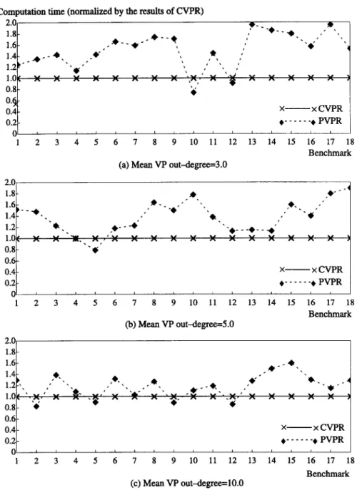
e . . . • PVPR i i i I @ - " @ - " "41' 1 2 3 4 5 6 7 8 9 10 11 12 13 (b) Mean VP out-degree=5.0 14 15 16 17 18 Benchmark 2.0 1.81 @, 1.6 1.4 @, • @" 1.0 "~, ~ , " ~ "a." , , , . . . . 4 , ' ' 4 k / 0.6[ 0.4 02 "0 I i I I I I I i i I I I I 1 2 3 4 5 6 7 8 9 10 11 12 13 14 (c) Mean VP out--degree=10.0 .4b "11 ~ " x x CVPR • . . . • PVPR 15 16 17 18 BenchmarkFigure 10. Comparison of the computation time between PVPR and CVPR.
Figure 8 depicts the c o m p u t a t i o n t i m e (on a logarithmic scale) of the S&P-based E B R M , D & G - b a s e d E B R M , P V P R , and C V P R algorithms for the benchmarks with different m e a n VP out-degrees. In the figure, we observe t h a t the P V P R and C V P R algorithms o u t p e r f o r m b o t h of the two versions of the E B R M algorithm for all benchmarks. Essentially, the superiority of the P V P R and C V P R algorithms has a pronounced increase with the complexity of the e m b e d d e d V P layout. It is worth noting t h a t c o m p u t a t i o n by P V P R and C V P R for realistic b e n c h m a r k s can be achieved in an order of a few minutes rather t h a n days required by b o t h E B R M algorithms. This justifies the practicability of the P V P R and C V P R algorithms for the efficient determination of the robustness of any given V P layout.
We further draw comparisons between the P V P R and C V P R algorithms in t e r m s of the n u m b e r of subproblems and the c o m p u t a t i o n t i m e in Figures 9 and 10, respectively. As shown in Figure 9, the n u m b e r of subproblems generated by P V P R is unsurprisingly lower t h a n t h a t generated by C V P R for all the benchmarks. As for the c o m p u t a t i o n time, C V P R o u t p e r f o r m s P V P R in most of t h e benchmarks, as shown in Figure 10.
5. C O N C L U S I O N S
This paper proposed the PVPR and CVPR algorithms for the efficient computation of TR in ATM VP networks by means of the variants of the path-based and cut-based partition methods, respectively. By partitioning based on the physical links and effectively reducing the number of generated subproblems, the two algorithms yield significantly low computational complexity compared to existing TR algorithms. Experimental results revealed that, compared to S&P-based and D&G-based EBRM algorithms, both the CVPR and PVPR algorithms exhibited superior performance for all the benchmarks. Moreover, the CVPR algorithm was shown to outperform the P V P R algorithm for most of the benchmarks in terms of computation time.
R E F E R E N C E S
1. C C I T T Recommendation 1.150, B-ISDN asynchronous transfer mode functional characteristics, Geneva, (1992).
2. C C I T T Recommendation 1.311, B-ISDN general network aspects, Geneva, (1992).
3. C C I T T Recommendation 1.363, B-ISDN ATM Adaptation Layer (AAL) specification, Geneva, (1993). 4. C C I T T Recommendation 1.361, B-ISDN ATM layer specification, Geneva, (1993).
5. J. Burgin and D. Dorman, Broadband ISDN resource management: The role of virtual paths, I E E E Commun.
Mag., 44-48, (September 1991).
6. H. Fujii and N. Yoshikai, Restoration message transfer mechanism and restoration characteristics of double- search self-healing ATM network, I E E E J. Select. Areas Commun. 12, 149-158, (January 1994).
7. R. Kawamura, K. Sato and I. Tokizawa, Self-healing ATM networks based on virtual path concept, I E E E J.
Select. Areas Commun. 12, 120-127, (January 1994).
8. Y.C. Chen and M.C. Yuang, A cut-based method for terminal-pair reliability, I E E E Trans. on Reliability 45 (3), (September 1996).
9. N. Deo and M. Medidi, Parallel algorithm for terminal-pair reliability, I E E E Trans. Reliability 41, 201-209, (June 1992).
10. A. Satyanarayana and A. Prabhakar, New topological formula and rapid algorithm for reliability analysis of complex networks, I E E E Trans. Reliability 27, 82-100, (June 1978).
11. W.P. Dotson and J.O. Gobien, A new analysis technique for probabilistic graphs, I E E E Trans. Circuits
Systems 26, 855-865, (October 1979).
12. S.N. Pan and J.D. Spragins, Dependent failure reliability models for tactical communications networks, In
Proc. Int. Conf. Commun., 1983, pp. 765-771.
13. L.B. Page and J.E. Perry, A model for system reliability with common-cause failures, I E E E Trans. Reliability 38, 406-410, (December 1989).
14. Y.F. Lam and V.O.K. Li, Reliability modeling and analysis of communication networks with dependent failures, I E E E Trans. Commun. 34, 82-84, (January 1986).
15. L.B. Page and J.E. Perry, Reliability of directed networks using the factoring theorem, I E E E Trans. Reliability 38, 556-562, (December 1989).
16. S. Rai, A. Kumar and E.V. Prasad, Computer terminal reliability of computer network, Reliability Engineer-
ing 16, 109-119, (1986).
17. S. Soh and S. Rai, CAREL: Computer aided reliability evaluator for distributed computing networks, I E E E
Trans. Parallel 0_4 Distributed Systems 2, 199-213, (April 1991).
18. D. Torrieri, An efficient algorithm for the calculation of node-pair reliability, In Proc. I E E E M I L C O M '91, November 1991, pp. 187-192.
19. D. Torrieri, Calculation of node-pair reliability in large networks with unreliable nodes, I E E E Trans. Relia-
bility 43, 375-377,382, (September 1994).
20. M.O. Ball, Computational complexity of network reliability analysis: An overview, I E E E Trans. Reliability 1=t35, 230-239, (August 1986).