家族發病時間資料之統計推論 - 文獻回顧

國 立 交 通 大 學

統計學研究所

碩 士 論 文

家族發病時間資料之統計推論

-文獻回顧

Statistical Inference

based on Familial Age-onset Data

- A Literature Review

研 究 生： 賴信宇

指導教授： 王維菁 博士

家族發病時間資料之統計推論-文獻回顧

Statistical Inference based on Familial Age-onset Data

- A Literature Review

研 究 生： 賴信宇

Student：Shin-Yu Lai

指導教授： 王維菁 博士

Advisor：Dr. Wei-Jing Wang

國 立 交 通 大 學 統 計 學 研 究 所

碩 士 論 文

A Thesis

Submitted to Institute of Statistics College of Science

National Chiao Tung University in partial Fulfillment of the Requirements

for the Degree of Master

in Statistics June 2010

Hsinchu, Taiwan, Republic of China

家族發病時間資料之統計推論

- 文獻回顧

學生： 賴信宇

指導教授： 王維菁 博士

國立交通大學

統計學研究所

摘

要

在本論文中，我們回顧有關分析家族發病時間的統計文獻。我們以統整的

架構，說明如何探討變數間的關聯性，與建立聯合分佈的方法。討論也包

含如何將解釋變數納入分析中的方法。在介紹完模式之理論意義與性質之

後，我們討論幾個文獻的實例，了解統計推論所牽涉到的問題與解決的方

法。

關鍵字：存活時間；發病時間；關聯模式

Statistical Inference based on Familial Age-onset Data

- A Literature Review

Student：Shin-Yu Lai Advisor：Dr. Weijing Wang

Institute of Statistics

National Chiao Tung University

Hsinchu, Taiwan

ABSTRACT

In the thesis, we review literature on statistical analysis of familial age-onset

data. A unified framework is provided to illustrate how statistical methods are

applied to investigate interesting scientific phenomenon. We discuss some

important association measures and several approaches to handling correlated

failure time variables. The extension to include the effect of covariates is also

introduced. Finally we discuss applications of these theoretical models to

biomedical data.

誌 謝

旻

賴信宇 謹誌于

國立交通大學 統計學研究所

西元 2010 年孟夏風城

Contents

Chapter 1

Introduction

...

1

1.1 Motivation and Background ... 1

1.2 Outline of the Thesis... 1

Chapter 2

Association Measures and Models

...

2

2.1 Association Measures ... 2

2.1.1 Pearson’s correlation... 2

2.1.2 Kendall’s tau ... 2

2.1.3 The odds ratio function ... 3

2.2 Model Construction... 4

2.2.1 Random effect approach ... 4

2.2.2 Conditional approach... 6

2.2.3 Copula modeling ... 8

Chapter 3

Mixed-effect Analysis for Familial Age-onset Data

...

12

3.1 Model for the Familial Study by Li and Thompson... 12

3.2 EM Algorithm for the Familial Study ... 14

3.3 Analysis for Breast Cancer Data... 16

3.4 Model for the Twin Study by Do et al. ... 16

3.5 Bayesian Inference for the Twin Study ... 19

3.6 Data Analysis for the Twin Study ... 21

Chapter 4

Copula Analysis for Familial Age-onset Data

...

23

4.1 Copula Model for the Familial Study by Andersen ... 23

4.2 Likelihood Analysis ... 24

4.3 Marginal Estimation ... 26

4.3.1 Likelihood-based approach ... 26

4.3.2 Martingale-based approach... 27

4.4 Association Estimation... 28

4.5 Data Analysis for Mortality in Twins ... 29

Chapter 5

Concluding Remarks

...

31

List of Tables

2.1 Two-by-two table at failure time

( , )t t1 2

………..3

3.1 Parameter estimates based on the model Cox-Gene and Cox-Gene-Envi

model………..………16

3.2 Result for time to menopause in twins for estimated regression coefficients

and estimated variance components.………..21

4.1 Result for mortality in twins for the gamma copula……….…..29

List of Figures

Chapter 1 Introduction

1.1 Motivation and Background

Age-at-onset is an important quantitative trait for many complex diseases. It is often chosen as the variable of interest in biomedical studies for assessing the relationship between the disease and environmental or genetic factors. Familial age-onset data are useful for detecting genetic and shared environmental effects. Specifically if such effects exist, we expect that the age-onset times of family members are correlated. Understanding the pattern of association may shed light on the disease etiology and is an important step useful for further scientific investigation.

An age-onset variable measures the time to onset of the disease and hence is a lifetime variable which can be analyzed under the context of survival analysis. In the thesis, we review some literature on familial age-onset data which are applied to different biomedical areas. For example, it has been recognized that both environmental and genetic risk factors play important roles in many human diseases such as breast cancer (Hsu, 1996)[11]_{, lung cancer (Li,}

1997)[12]_{, dementia, and heart disease. The purpose of the thesis is to provide a unified}

framework to illustrate how statistical methods are applied to investigate these scientific problems.

1.2 Outline of the Thesis

Let ( ,T T_{1 2},,T_k) be the age-onset variables for k members in a family. Note that T _i

and T for i_j  are often correlated. In Chapter 2, we focus on the simplified case with j k=2. Several association measures for ( ,T T and different approaches to constructing the _{1 2}) joint model are discussed. In Chapter 3, we illustrate how these ideas in Section 2.2.1 and 2.2.2 are applied to analyze familial age-onset data with mixed-effect. Copula analysis for familial age-onset data will discuss in Chapter 4. Chapter 5 contains concluding remarks.

Chapter 2 Association Measures and Models

In many biomedical applications, research interest focuses on the dependence relationship between two variables. Let T and ₁ T be two failure times of interest. Define ₂

the joint survival function as S t t( , )_{1 2} Pr

_

T₁ t T₁, ₂ t₂

_

and the corresponding density function as 2 1 2 1 2 1 2 ( , ) ( , ) S t t f t t t t  

  . In this chapter we review some commonly-seen association measures. Then we discuss different approaches to constructing models which describe the dependence structure.

2.1 Association Measures 2.1.1 Pearson’s correlation

Pearson’s correlation is perhaps the most popular measure of correlation which is defined as: 1 2 1 2 ( , ) ( ) ( ) Cov T T Var T Var T  

This measure reflects the degree of linear relationship between two variables. Recall that

1  1

   and its sign describes the direction of association and its value measures the degree of association. Since  is defined in terms of moments, it is not robust which implies

that it may not be very suitable for skew distributions.

2.1.2 Kendall’s tau

Let (T T_i1, _i2) and (T T_j1, _j2) (i j) be independent realizations from ( ,T T_{1 2}) . The ( , )i j pair is called “concordant” if (T_i1T_j1)(T_i2T_j2)0 and “discordant” if

1 1 2 2

(T_i T_j )(T_i T_j )0. The population version of Kendall’s tau is defined as the difference of concordance and discordance probabilities between pair ( , )i j . If T and ₁ T are continuous, ₂



1 1 2 2





1 1 2 2



Pr (T_i T_j )(T_i T_j ) 0 Pr (T_i T_j )(T_i T_j ) 0

        

It is easy to see that  1  1 and, if ( ,T T are independent, _{1 2})  0. Kendall’s tau is known as a rank invariant measure since its value does not change as long as the marginal ranks remain the same. Estimation of  has been discussed in Wang and Wells (2000)[18]_.

2.1.3 The odds ratio function

The above two measures,  and  , describe global association. For failure time

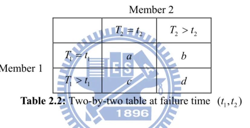
variables, one may be interested in more detailed information about the dependence structure. Consider the following two-by-two table:

2 2 T t T₂ t₂ 1 1 T  t a b 1 1 T  t c d

Table 2.2: Two-by-two table at failure time ( , )t t_{1 2}

If the failure times are discrete, the magnitude of association at time ( , )t t_{1 2} can be measured by the odds ratio:

1 1 2 2 1 1 2 2 1 1 2 2 1 1 2 2 Pr( , ) Pr( , ) Pr( , ) Pr( , ) T t T t T t T t ad bc T t T t T t T t          . (2.1a)

For continuous distributions, Oakes (1989)[15] _{proposed the following cross-ratio function:}











2 1 2 1 2 1 2 * 1 2 1 2 1 1 2 2 ( , ) ( , ) ( , ) ( , ) ( , ) S t t S t t t t t t S t t t S t t t          . (2.1b)

When ( ,T T are independent, _{1 2}) * 1 2

( , ) 1t t

  for all ( , )t t_{1 2} . Departure from 1 implies that association exists. This measure is useful for assessing how the level of association varies with time ( , )t t_{1 2} .

Member 2

2.2 Model Construction

We discuss different approaches to constructing the joint distribution of ( ,T T . _{1 2}) 2.2.1 Random effect approach

It is assumed that there exists some random effect denoted as  such that, given  , T 1

and T are independent. This implies that the dependence is fully explained by ₂  which is

assumed to be one-dimensional to ensure identifiability. Depending on the context,  may

represent traits which are common for the two variables. Due to conditional independence, it follows that

1 2 1 1 2 2

( , | ) ( | ) ( | )

S t t  S t  S t  .

It remains to determine how  affects T . Usually a common assumption is that the j

random effect acts multiplicatively on the hazard, so that _j( )t _0j( )t , where j 1, 2 and

0j( )t

 is the hazard function for the baseline group with  1 . Accordingly

0

( ) ( )

j t  j t

   and S t_j( | ) S_0j( )t . The conditional joint survival function is then

1 2 01 1 02 2

( , | ) ( ) ( )

S t t  S t S t .

Because  is not observable, to obtain the unconditional survival function, one needs to

‘integrate out’  . Assume that  has the density g( ) . It follows that

 





01 1 02 2 1 2 1 2 0 ( ) ( ) 0 1 2 ( , ) ( , | ) ( ) ( ) ( , | ) t t S t t S t t g d e g d E S t t           _{  }   





(2.2) which is the Laplace transform of g( ) evaluated at s 01( )t1  02( )t2 . Thus we can

denote

1 2

( , )

S t t  £_g

_

₀₁( )t₁  ₀₂( )t₂

_

, (2.3) where £_g denotes the Laplace transform, £ ( )g s e s g( )d

 _{ } 

Example: Gamma frailty

A convenient assumption adopted in a number of literatures is that  has a gamma

distribution. This distribution has the appropriate range (0, ) and is mathematically tractable. The density of a gamma distribution with parameters  and  is

1

( ) ( )

g  e 

  .

The mean and variance are E( )   and Var( )  2. It is often convenient to make the additional assumption E( ) 1  . To achieve this, we can set   1 / such that

( )

Var  . Note that the Laplace transform of the gamma density is

£ 1/ (1/ ) ( ) (1/ ) s s            .

Using this result, we obtain that

1 2 ( , ) S t t £_g

_

₀₁( )t₁  ₀₂( )t₂

_

1 01 1 02 2 1 1 ( )t ( )t              



01( )t1 02( ) 1t2



1          . _(2.4)

From the expression of the joint survival function, we can obtain





1 1( )1 ( , 0)1 01( ) 11 S t S t   t   , where ₀₁( )t₁ S t₁( )₁   . 1 It follows that





1/ 1 2 1 1 2 2 ( , ) ( ) ( ) 1 S t t  S t  S t    . _(2.5) The above model was first introduced by Clayton (1978)[5] _{who derived this family based on}

a different approach. A useful result for the family of Gamma frailty is

2      . (2.6) ■

In addition to the random effect, there often exist observed covariates which also account for the existence of heterogeneity and dependence (Docrocq and Casella, 1996)[7]_{. Let}

j

Z be

observed covariates for T . If the multiplicative effect on the hazard is still adopted, then we _j

have 0 ( | , ) ( | ) j tj Zj j tj Zj    . (2.7) Assume that _0j( |t_j Z_j) follows the Cox proportional hazards model with



'



0j( |tj Zj) 0( ) exptj jZj

    , _(2.8)

where _0j( )t is the hazard function for the baseline group with   and 1 Z  . Due to _j 0 conditional independence, the survival function follows that

1 2 1 2 1 1 1 2 2 2

( , | , , ) ( | , ) ( | , )

S t t Z Z  S t Z  S t Z  . Then the un-conditional survival function is given by

1 2 1 2 1 1 1 2 2 2 0

( , | , ) ( | , ) ( | , ) ( )

S t t Z Z 

_

S t Z  S t Z  g  d . _(2.9) With the gamma frailty, we have





1/ 1 2 1 2 1 1 1 2 2 2 ( , | , ) ( | ) ( | ) 1 S t t Z Z  S t Z  S t Z    , _(2.10) where ( | ) ₀ ( )exp( 'jZj) j j j j j S t Z S t  (j 1, 2). 2.2.2 Conditional approach

A conditional approach, from its literal definition, is to construct a joint model from two components: T T and ₁| ₂ T (or ₂ T T and ₂| ₁ T ). However such a straightforward derivation ₁

is order dependent. There exists a better way of model construction which turns out to be exchangeable in the two coordinates. Consider two conditional hazard functions:



1 1 1 1 1 2 2



1 1 2 2 ₀ Pr [ , ) | , ( | ) lim h T t t h T t T t t T t h         and



1 1 1 1 1 2 2



1 1 2 2 0 Pr [ , ) | , ( | ) lim h T t t h T t T t t T t h         . Notice that 1 1 2 2 2 2 1 1 1 2 1 1 2 2 2 2 1 1 ( | ) ( | ) ( , ) ( | ) ( | ) t T t t T t t t t T t t T t            (2.11)

which does not depend on the order of conditioning. The parameter ( , )t t_{1 2} measures the degree of association between T and ₁ T at bivariate time ₂ ( , )t t_{1 2} . Also notice that

* 1 2 1 2

( , )t t ( , )t t

  in (2.1).

Clayton (1978)[5] _{assumed that}

1 2

( , )t t c

 

which implies that the dependence level does not varies with time. The model proposed for all t and ₁ t ₂ 1 2 1 2 1 2 2 1 ( , ) ( , ) ( , ) ( , ) t t f t t S t t c

_

 f u t du

_

 f t v dv.

From theassumption, one obtains the following second-order partial differential equation:







 



2

1 2 1 2 1 2

1 2 1 2

log ( , ) log ( , ) log ( , )

( 1) 0 S t t S t t S t t c t t t t              .

Consequently, the solution of the differential equation is given by



( 1) ( 1)



1/( 1)

1 2 1 1 2 2

( , ) ( ) c ( ) c 1 c

S t t  S t   S t      . _(2.12) To include covariates, suppose that there exists covariates Z which is common to both

1 T and T so that ₂ ' 1 2 ( ,t t | )Z c Z( ) exp( Z)     , _(2.13)

where  is a parameter. Also there exist covariates Z and ₁ Z which are specific to ₂

marginal distributions of T and ₁ T as before. As a result, we have ₂

   



( ) 1 ( ) 1



1/ ( ) 1 1 2 1 2 1 1 1 2 2 2 ( , | , ) ( | ) ( | ) 1 c Z c Z c Z S t t Z Z S t Z S t Z          . _(2.14)

2.2.3 Copula modeling

Copula models have been frequently adopted in the literature due to their nice properties. We first give the formal definition.

Definition of the copula function

Copula, expressed as C is a n-dimensional function having uniform marginal distribution that satisfies the following three conditions:

1. C:[0,1]n [0,1];

2. C is a grounded and n-increasing function;

3. C has margins C that satisfies _i C_i(u)C(1,...,1,u,1,...,1)u, u [0,1]. ■

Based on the above definition, it is clear that a copula function is the joint probability distribution for uniform random variables. The following theorem expands the application of copula functions.

Theorem 2.1 (Sklar’s Theorem)

If F ( ) is an n-dimensional cdf (or survival function) with continuous

marginsF ,...,₁ F_n, we can find the following unique copula representation:





1 1 1

( ,..., _n) ( ),..., _n( _n)

F x x C F x F x .

■

That is for multivariate random variables X _j (j1,..., )n with the marginal function F  , _j( )

we can construct their joint model under the copula structure.

Now we consider the special case of only two failure times. The paper by Genest and MacKay (1986)[9] _{derived useful properties of the bivariate family. The bivariate copula}

function can be written as





1 2 1 1 2 2

( , ) Pr , (0 _j 1)

C u u  U u U u u 

where (U U₁, ₂) are uniform (0,1) variables marginally and 2

( , ) : [0,1] [0,1]

C   

characterizes the dependence structure. Note that if C u u( ,_{1 2})u u_{1 2} for all 0u_j  1 (j 1, 2), U and ₁ U are independent. ₂

Let ( ,T T_{1 2}) be a pair of continuous failure times. In applications of lifetime data analysis, the copula structure is usually imposed on the survival function such that

















1 2 1 1 2 2 1 1 1 1 2 2 2 2 1 1 1 2 2 2 1 1 2 2 ( , ) Pr , Pr ( ) ( ), ( ) ( ) Pr ( ), ( ) ( ), ( ) . S t t T t T t S T S t S T S t U S t U S t C S t S t          

where S T _j( )_j (j 1, 2) is distributed as Uniform(0,1), and



1 1



1 2 1 1 2 2

( , ) ( ), ( )

C u u S S u S u



was called as the “copula models” by Sklar (1959)[17]_{. Models in the copula family allow for}

separate investigation on the marginal behaviors and the dependence structure which is often the main interest. As mentioned earlier, when T and ₁ T₂ are independent,

1 2 1 1 2 2

( , ) ( ) ( )

S t t S t S t and C u u( ,_{1 2})u u_{1 2}. If T₁ T₂, S t t( , )_{1 2} S t₁( )₁ S t₂( )₂ such that

1 2 1 2

( , )

C u u u u which is the case of maximal dependence. The copula function C u u( ,_{1 2}) is usually parameterized as C u u_( ,_{1 2}), where the parameter  measures the association

between ( ,T T . Note that _{1 2})  is related to Kendall’s  , then

2 1 2 1 2 1 2 1 2 ( , ) ( ) 4 C u u( , ) C u u du du 1 u u         



. (2.16) Semi-parametric inference of the copula parameter without specifying the marginal distributions has received substantial attentions in the literature.

The Archimedean copula (AC) family, which is a sub-class of the copula family, is attractive due to its nice analytical properties. For an AC model, the bivariate copula function

1 2

( , )





1 1 2 1 2 ( , ) ( ) ( ) C u u_ _ _ u _ u   for u u ₁, ₂ [0,1], (2.17) where  _( ) : [0,1][0, ] is a univariate function which has two continuous derivatives

satisfying _(1)0, ( )t ( )t 0 t          and 2 2 ( ) ( )t t 0 t        

 . AC models have the nice feature that the bivariate relationship can be summarized by the univariate function

( )



  . Recall the cross-ratio function defined previously:

2 * 1 1 2 2 1 1 2 2 1 2 1 2 1 1 2 2 1 1 1 2 2 2 {Pr( , )}{ Pr( , ) / } ( , ) { Pr( , ) / }{ Pr( , ) / } T t T t T t T t t t t t T t T t t T t T t t                  .

From Oakes (1989), an AC model has the nice property that





* 1 2 1 2 ( , )t t S t t( , )   , ( )v v ( )v ( )v

     is a univariate function. A special property of the Clayton model

reflects in its local odds ratio which can be expressed as *( , )t t_{1 2}  and 

_

S t t( , )_{1 2}

_

does not depend on ( , )t t_{1 2} . In AC model, Kendall’s tau has the analytic expression:

1 0 ( ) 4 1 ( )d         



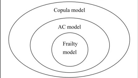
. If 1

is a Laplace transform of some distribution, Archimedean copula models reduce to proportional frailty models.

For the frailty model, the bivariate joint survival function can be expressed by integrating out the frailties with respect to the frailty density









1 1 2 ₀ 1 2 01 1 0 2 2 2 ( , ( , ) ( , | ) ( ) ex ) ) , ) p ( ( S t t S t t g d E t S t t t          _     _



(2.19) where  and ₀₁  are the cumulative hazard functions conditional on ₀₂  . Furthermore,

the marginal survival function for each of the two imaging techniques can be obtained by having the age-onset time for the other diagnostic technique equal to zero in equation (2.19)





1 0 ( )s L s( ) E exp( s ) exp( s ) ( )g d           

_

 . _(2.18)

and thus S t_j( )L



_0j( )t



. It follows that _0j( )t L1



S t_j( )







S t_j( )



   .

We can draw the relationship of sub-families for bivariate association model:

Figure 2.1: Relationship among copula models Frailty

model AC model Copula model

Chapter 3 Mixed-effect Analysis for Familial Age-onset Data

In this chapter, we illustrate the application of random effect approach in analysis of familial data. Since there also exist observed covariates, the method becomes a mixed-effect approach.

3.1 Model for the Familial Study by Li and Thompson

For many common complex diseases, major susceptible genes which account for familial aggregation of the disease have been identified. For example for breast cancer, P53 (Malkin et

al., 1990)[13]_{, BRCA1 (Miki et al., 1994)}[14] _{and BRCA2 (Wooster et al., 1994)}[19] _{are thought to}

cause inherited breast cancer. It has been observed that carriers with susceptible gene tend to have earlier onset ages of the disease than non-carriers.

Li and Thompson (1997)[12] _{modified the Cox model to analyze familial age-onset data.}

Let T be the onset age for the _ij jth individual in the thi family for j 1, ,k_i and

1, 2, ,

i  N . Observed covariates for an individual include measurable genotypic information denoted as g and other observed covariates denoted as _ij Z . It is important to _ij

note that ( ₁, , )

i

i ik

g  g are correlated which can be modeled by employing related biological

knowledge. In this paper, it is assumed that a single major Mendelian diallelic locus governs disease susceptibility. Assume that there are two alleles at this locus and denote them by A and

a, where A is the dominant disease allele with allele frequency. The genotypic covariate g _ij

is coded as a categorical variable with three levels (aa), (aA), (AA). Let the probability of

A=Pr( )A q which measures allele frequency in the population. The joint probability

1

Pr( , , )

i

i ik

g  g can be determined by Mendelian heredity law which has is the hierarchical

property that the parents’ information can determine the offspring’s probability.

or

ij ij

S I g_  Aa AA_{ . The first objective is to model}  T based on (_ij S Z_ij, _ij). Li and

Thompson (1997)[12] _{first considered the following Cox-Gene model:}

0

( | , ) ( ) exp( ' )

ij t Z Sij ij t Zij Sij

   

(3.1a) where ₀( )t is the hazard for the baseline group with g_ij aa and Z _ij 0,  measures

the effect of Z on the hazard and _ij  measures the effect of having genotype “A” on the

hazard. It is important to mention that the model in (3.1a) is a semi-parametric structure since the baseline hazard function is not specified. Compare with equation (2.8) in Section 2.2.1, (3.1a) add S into the covariate components, where _ij S_ij is the presence of the dominate

gene and it is observable.

To allow for the dependence among k family members, the approach of random effect _i

is also adopted. Assume that  denotes unobserved random effect within family i and it _i

affects the hazard of T in a multiplicative form. The following model is referred as the _ij

Cox-Gene-Envi model: 0 ( | , , ) ( ) exp( ' ) ij t Z Sij ij i t i Zij Sij       . (3.1b) Through the influence of  on _i T , _ij ( ₁, , )

i

i ik

T  T become correlated and the source of

association may be explained by shared environmental effects. It is further assumed that

1 1 ~ , iid i gamma           

  with the density

(1 1) 1 exp( ) ( ) (1 ) f            

and E( ) 1  and Var( )  . Note that large value of  reflects high heterogeneity in

families which corresponds to larger association among family members.

The paper also discusses how to model the distribution of Pr



G_i



which depends on the family structure and is calculated here under the assumptions of random mating and

Mendelian segregation which however is not our expertise. Nevertheless we summarize the basic principle. For any genotypic configuration ( ₁,..., )

i

i  gi gik

G , one can write













founder nonfounder Pr Pr Pr , ij ij i il ij m f il ij g g g g 

_

_

G (3.2) where Pr

 

g_il is the genotypic frequency and is a function of the allele frequency

Pr( )A q and Pr



,



ij ij

ij k f

g g g is the Mendelian transmission probability given by parents.

The decomposition of (3.2) depends on how members in a family are selected.

3.2 EM Algorithm for the Familial Study

Data in this example can be denoted as (Xij_,ij,g Zij_, ij, )i for j 1,...,ki and

1,...,

i N, where X_ij T_ijC_ij min( ,T C_{ij ij}) and C_ij is the censoring time. Recall that

or

ij ij

S I g_  Aa AA_ and Pr(G is the probability of the all members in the ith family _i) with the gene frequency of A is q. Consider the full model in (3.1b). If  is observed, the _i

contribution for ith family to likelihood function can be written as

1 , , 1 ( | ) ( | ) Pr( ) i ij ij ij ij ij ij i k Z S ij i Z S ij i i j f x   S x   



G G





, , 1 ( | ) exp ( | ) Pr( ) i ij ij ij ij ij i k Z S ij i Z S ij i i j x  x     

_

 G G

which is a function of (₀( ), , , )t   q . To include the randomness of  , the likelihood _i

component for ith family becomes





, , 1 0 ( | ) exp ( | ) ( ) Pr( ) i ij ij ij ij ij i i k i S Z ij i S Z ij i i i i j L x  x d                    







G G

which is a function of  (₀( ), , , , )t    q . The parameter  measures the effect of Z _ij

and  measures the unobserved family-specific effect. The full likelihood function can be written as





, , 1 0 1 ( | ) exp ( | ) ( ) Pr( ) i ij ij ij ij ij i i k N S Z ij i S Z ij i i i i i j x  x d                    









G G

which however is difficult to analyze directly.

The idea of EM algorithm is applied to simplify the likelihood analysis. Temporarily assuming that ( , )G  are also observed. The complete data log-likelihood l is given by _c









0 , , 1 1 1 1 1 1 ' ' 0 0 1 1 1 , , , , , , ,

log ( | ) ( | ) log ( ) log Pr( )

log ( ) exp( ) ( ) exp( )

i i ij ij ij ij i i i c c k k N N N N ij S Z ij i g Z ij i i i i j i j i i G k k N ij ij i ij ij i ij ij ij i j i j l l q X x x G x Z S x Z S                                      _{ }       















G









1 1 1 1 1 ' ' 0 0 1 1 1 1 1 1 log ( ) log Pr( ) log exp( )

( ) exp( ) log ( ) exp( )

log ( ) log Pr( ) i i i i i N N N i i i i G k N ij i ij i j k k N N i ij ij ij ij ij ij i j i j N N i i i i G G S x Z S x Z G                             _{ }            _{ }  





















 





 

 

1 2 0 3 4 l  l  , , l  l q

which nicely separates the parameters.

Since ( , )G  are not directly observed, the E-step involves replacing ( , )G  by E ( ,_ G  X, ) through Monte Carlo approximation. The evaluation of expectations for the E-step requires the conditional distribution of  , the joint conditional distribution of G, and the joint conditional distribution of ( , )G  , given the observed data ( , )X  . Specifically the

( , , ) ( ) ( ) ( , , ) ( , , ) ( ) ( ) P X P f f X P X P f d                  

 

G G G G G G . (3.3) It is still computationally difficult to evaluate the denominator of the above equation. The authors suggest to apply the Gibbs sampler for implementation. Let _ij _iexp(S_ij) where

I( , )

ij ij

S  g  Aa AA such that ˆ_ij E(_ij) . Then E( )l_c will be adopted as the target

likelihood. To compute E( )l_c we need E (_ S X_ij , ), E (_ S_ij_i X, ), E ( ),_ _i and

i

E (log )_  , the expectations are computed by Monte Carlo approximation to complete the E-step of our algorithm. Finally E



l q₄( )



is maximized over q, E



l₃( )



over , and





1 2 0

E_l ( ) l  , , ( )t _ over



  , , ₀( )t



.

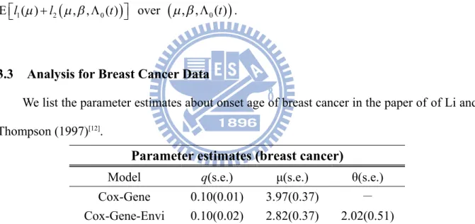
3.3 Analysis for Breast Cancer Data

We list the parameter estimates about onset age of breast cancer in the paper of of Li and Thompson (1997)[12]_.

Parameter estimates (breast cancer)

Model q(s.e.) μ(s.e.) θ(s.e.)

Cox-Gene 0.10(0.01) 3.97(0.37) － Cox-Gene-Envi 0.10(0.02) 2.82(0.37) 2.02(0.51)

Table 3.1: Parameter estimates based on the model Cox-Gene and Cox-Gene-Envi model The Cox-Gene model gives a significant estimate of genetic effect. The Cox-Gene-Envi model results in significant major gene effect and also strong intra-family correlation as measured by the variance of the Gamma frailty, indicating that familial aggregation of breast cancer may be due to both gene segregation and shared familial risk.

3.4 Model for the Twin Study by Do et al.

diseases. Monozygotic (MZ) twins are genetically identical while dizygotic (DZ) twins, on the average, have half their genes in common. Therefore the association between MZ twins should be stronger than that between DZ twins. Do et al. (2000)[6] _{compared the time to}

menopause for two types of twins. Denote (T T_i1, _i2) as the onset ages for the twin in the ith family for i1, 2,,N. Let Z be the observed covariates for twin j of the _ij ith family

which include the birth year and the age at menarche (both continuous), and binary variables including smoking (0 non-smokers), parity (0 fewer than 2 children) and education (0 no university education).

Modeling involves two aspects. One refers to modeling how Z affects _ij T and the _ij

other is related to the dependence structure between T and _i1 T given _i2 Z and _i1 Z . In _i2

Section 2.2.1, (2.7) and (2.8) have the form that covariates Z and the random effect _ij

component  affect _i T have a proportional hazard model. And the baseline hazard rate _ij

0( )t

 is possibly un-specified.

For the former issue, Do et al. adopted a parametric approach. Specifically the marginal distribution of T given _ij Z is modeled by a Weibull distribution with _ij

1 ( ) ij exp( ij ) ij Z f t te e t    , (3.4) where  is the shape parameter and  is the scale parameter depending on ij Z . An ij

additional random-effect component is imposed on the scale parameter  such that _ij

'

log_ij  Z_ij m_ij,

(3.5) where Z is observed covariates and _ij m denotes the unobserved covariate. The random _ij

effect m affects individual heterogeneity which cannot be explained by _ij Z and also _ij

2.2.1, the random effect component has a proportional effect on the marginal hazard functions. However in (3.4), the random effect has a proportional effect on the scale parameter  . _ij

The approach of Do et al. (2000)[6] _{was motivated by the covariance component analysis}

proposed by Eaves et al. (1978)[8] _{who proposed to decompose the total phenotypic covariance}

into genetic and environmental components. Here the sources of co-variation are classified as follows:

Additive genetic factors (A) are the effects of genes taken singly and added over multiple

loci;

Shared environmental effects (C) are the common environmental effects.

Different structures are imposed on m for the two types of twins. Accordingly Do et al. _ij

(2000)[6] _{proposed the following two sub-models of}

ij

m for MZ and DZ twins. Specifically

the sub-model for MZ twins is

' log_ij( )Z Z_ijm_i, (3.6a) where m_i1m_i2 m_i and 2 2 ~ N(0, ) i A C

m   . The sub-model for DZ twins is given by

'

log_ij( )Z Z_ij_i_ij,

(3.6b) where m_ij _i_ij, _i _ij,  is a random effect common for the twin pair such that _i

2 2 1 2 ~ (0, ) i N A C    ;

and  is a random effect for individual j such that _ij

2 1 2 ~ (0, ) ij N A   .

Notice that shared environmental effects contribute  to the variance of _C2 m for both types _ij

of twins. Genetic effects contribute  to the variance of _A2 m which however reveals _ij

2 A

 is common for a twin. On the other hand, DZ twins have half their genes in common

while, the other half genes, are different. Thus 1 2

2 is common for the twin pair and A 2 1 2 A

is left to model the variance of  which measures the unobserved effect due to half _ij

different genes. In the next section, we will illustrate how the parameters are estimated which utilize Bayesian techniques.

3.5 Bayesian Inference for the Twin Study

Consider the twin data in Section 3.4. Denote onset times as T

_

T₁,,T TK; K₁,,TN

_

where T_i (T T_i1, _i2) and the first K observations are for MZ twins and the last NK

ones are for DZ twins. Model (3.4) and (3.5) gives the form of ( )

ij

Z

f t . The likelihood

contribution for ith MZ twin is given by

1( 1| ) 2( 2| ) 1( ) i i i Z i i Z i i i i m f t m f t m  m dm



(i1,...,K), (3.7a) where based on (3.6a),

2 1 1 ( ) exp 2 2 MZ MZ x x      _ _   _{ },

and _MZ _A2_C2. Similarly the likelihood contribution for ith DZ twin is given by

1 2 2 1 1 1 2 2 2 3 1 3 2 1 2 ( | , ) ( | , ) ( ) ( ) ( ) i i i i i Z i i i Z i i i i i i i i i f t f t d d d                

  

_(3.7b)

where iK1,...,N and based on (3.6b),

2 2 1 ( ) exp 2 2 _{DZ DZ} x x      _ _   _{ }, 2 3 1 ( ) exp 2 2 _{E E} x x      _ _   _{ }, and 1 2 2 2 DZ A C    and 1 2 2 E A

  . Knowledge of genetics is applied to construct the

DZ twins. Note that 2

2( )

A MZ DZ

     and 2 2

C MZ A

    . The whole likelihood function

can be written as ( ) f T 1 1 2 2 1 1 ( | ) ( | ) ( ) i i i K Z i i Z i i i i i m f t m f t m  m dm  

_{ }

1 2 2 1 1 1 2 2 2 3 1 3 2 1 2 1 ( | , ) ( | , ) ( ) ( ) ( ) i i i i i N Z i i i Z i i i i i i i i i i K f t f t d d d                   

_{   }

.

Direct likelihood estimation is an impossible task. Fortunately the underlying Bayesian structure is useful for implementing modern simulation techniques for parameter estimation. Denote  as the vector of parameters and T be the observed data. Denote ( ) as the prior distribution of the parameter with some random effect. The likelihood function refers to

( | )

f_Z T  . The Posterior density is given by

( | ) ( ) ( | ) ( ) f f     Z   Z T T T . (3.8)

It is difficult to derive the distribution of ( T| ) analytically. However, the algorithm of Gibbs sampling allows one to obtain many random samples from ( T| ) without knowing its form which can be further utilized for parameter estimation. Now we apply the Gibbs sampling algorithm to the aforementioned example.

Denote  ( , , ,   _MZ,_DZ,_E) and (0) be the initial value. To obtain each component of ( )r

 , the estimated value in rth step, the following algorithm is suggested: - draw ( )r from ( 1) ( 1) ( 1) ( 1) ( 1) ( | , r , r , MZr , DZr , Er )             T - draw ( )r  from ( ) ( 1) ( 1) ( 1) ( 1) ( | , r , r , r , r , r ) MZ DZ E            T - draw ( )r from ( ) ( ) ( 1) ( 1) ( 1) ( | , r , r , MZr , DZr , Er )           T - draw ( )r MZ  from ( ) ( ) ( ) ( 1) ( 1) ( | , r , r , r , r , r ) MZ DZ E        T   - draw ( )r DZ  from ( ) ( ) ( ) ( ) ( 1) ( | , r , r , r , r , r ) DZ MZ E       T  

- draw ( )r E  from ( ) ( ) ( ) ( ) ( ) ( | , r , r , r , r , r ) E MZ DZ   T      .

The above successive procedure is repeated for r = 1,2,3, … until some convergence criterion is reached. Denote ( )L  (( )L ,( )L ,( )L ,( )_MZL ,( )_DZL ,_E( )L ) as the sample value obtained in the Lth step. Based on Casella and George (1992)[4]_{, as long as}

L is large enough, ( )L

 will be an effective random realization of  from ( T| ). We can generate

M independent Gibbs sequences of length L, which would yield an approximate iid sample from posterior density ( T| ). Based on the sample, we can estimate  by the sample mean. For example to estimate  , we can take the sample average of ( )L based on M observations.

Notice that ( , )  measures the effect of observed covariates while ( _A2, _C2) reflect genetic and environmental influences on the variation of the scale parameter. Generally speaking, larger variation corresponds to higher association. To be more specific, large variation in the population means that individuals in different families are unalike. These unobserved characteristics, on the other hand, are similar to twin members in each family which explains their association.

3.6 Data Analysis for the Twin Study

We list the partial result for time to menopause in twins for estimated regression coefficients and estimated variance components in the literature of Do et al. (2000)[6]_.

Gibbs sampling approach parameter estimates

Covariate Coefficient β Robust s.e.(β) 95% CI of β (a) Mean effects

Year of birth ﹣0.029 0.0035 (-0.036,-0.023)*

Smoking 0.138 0.0788 (-0.187, 0.293)

University education ﹣0.397 0.1400 (-0.676,-0.123)*

Menarche ﹣0.024 0.0204 (-0.063, 0.015)

(b) Variance components 2 A  _{0.730 0.3290 ( 0.129, 1.410)*} 2 C  _{0.011 0.2400 ( 0.456, 0.489)}

Table 3.2: Result for time to menopause in twins for estimated regression coefficients and estimated variance components

Chapter 4 Copula Analysis for Familial Age-onset Data

In the previous chapters, we have discussed how familial data are analyzed by mixed-effect models. In this chapter, we consider the application of copula models in analysis of familial age-onset data. Properties of copula models are introduced in Section 2.2.3 and here they are applied to study the mortality of twins. In genetic studies, association studies of twins provide useful information about the effect of heredity on the problem of interest. Anderson (2005)[3] _{analyzed the lifetime of Danish twins born in the period 1881–1930 which}

reveal information about how genetics affect human’s lifetime. The data were divided into six groups: MZ males, DZ males, UZ (unknown zygosity) males, MZ females, DZ females and UZ females, where the twins are of the same sex and both were alive at the age of 15. Subjects were followed until 1980, and their mortality has been registered.

4.1 Copula Model for the Familial Study by Andersen

Let ( , )T T be the lifetimes of twins. Let _{1 2} Z be the covariate for _j T . In the data, _j Z _j

represents the continuous variable ‘year of birth minus 1900’/100. The explanatory variable was chosen because people born later tend to live longer due to the advance of medicine and improvement of general health. The effect of Z on mortality is modeled through _j _j( )t

which is the marginal hazard function of T (_j j 1, 2). Specifically the Cox PH model is

assumed:

0

( | ) ( ) exp( )

j t Zj t jZj

   ,

where the baseline intensity ₀( )t is an unknown baseline hazard function of t and  is _j

the vectors of parameters. The cumulative baseline hazard function is given by

0( ) ₀ 0( ) t

t  s ds

 

_

.

Besides the interest in  which measures the marginal covariate effect on _j T , the _j

association between the two variables is also of interest. Larger association implies that mortality is more affected by genetics. Denote S t t( , )_{1 2} Pr(T₁t T₁, ₂ t₂) as the joint survival function of ( , )T T . Without covariates, when _{1 2} ( , )T T come from the C1 2  copula,

the joint survival function can be parameterized as S t t( , )_{1 2} C_



S t₁( ),₁ S t₂( )₂



, where

2

:[0,1] [0,1]

C  characterizes the dependence structure and  measures the degree of

association. In presence of covariates, the copula model can be written as





1, 2( , )1 2 1( |1 1), 2( |2 2)

Z Z

S t t C_ S t Z S t Z ,

where under the Cox model, ( | ) ₀ ( )exp( jZj)

j j j j j

S t Z S t   and S_0j( )t Pr(T_j t Z| _j). Note that  does not depend on the covariates implies that the degree of association is the same

for each covariate group. For an Archimedean copula model, we can write

Data in presence of right censoring consist of (X_i1,X_i2, _i1, _i2,Z_i1,Z_i2) for i 1, ,N, where X_ij min(T C_ij, _ij), _ij I X( _ij T_ij) and (C C_i1, _i2) denote the censoring variables for

1 2

(T T_i , _i ). Now we discuss how to estimate  and  (_j j 1, 2).

4.2 Likelihood Analysis

In absence of covariates, we can write









1 1 2 2 1 1 1 1 2 2 2 2 1 1 2 2 1 2 Pr( , ) Pr ( ) ( ), ( ) ( ) Pr( , ) , . T t T t S T S t S T S t U u U u C_ u u         

In presence of covariates, let Uij S Tj( ij|Zij), where S t Zj( | j)Pr(Tj t Z| j). If the form













1 2 1 , ( , )1 2 1( |1 1) 2( |2 2) . Z Z S t t _ _ S t Z _ S t Z

of S  is completely specified and there is no censoring, we can construct the likelihood _j( ) function of  ( ,  _{1 2}, ) as 1 2 1 ( ) ( , ) N i i i L c u u_  

_

, where





2 1 2 1 2 1 2 , ( , ) C u u c u u u u    

  and uij S tj( |ij Zij). Now we establish the likelihood in presence of censoring. Observed data can be written as (X_i1,X_i2, _i1, _i2,Z_i1,Z_i2), we can obtain: U_ij S X_j( _ij|Z_ij) for i 1, ,N and j 1, 2. Now we discuss when does U_ij

relate to U . As _ij   , _ij 1 Uij Uij; as   , we have ij 0 Xij Tij and Uij Uij since S  j( )

is a decreasing function. Accordingly, when ( _i1, _i2)(1,1), (u u _i1, _i2)(u u_i1, _i2) and we assign c

_

u ui₁,i₂

_

to the likelihood; when ( i1, i2)(1, 0), ui1  , ui1 ui2   and we ui2

assign C_(10)(u u _i1, _i2) to the likelihood; when ( _i1, _i2)(0,1), u_i1  , u_i1 u_i2   and we u_i2

assign C_(01)(u u _i1, _i2) to the likelihood; when ( _i1, _i2)(0, 0), u_i1  , u_i1 u_i2   and we u_i2

assign C u u_( _i1, _i2) to the likelihood, where (10) _{1 2 1 2}

1 ( , ) ( , ) C u u C u u u      and (01) 1 2 1 2 2 ( , ) ( , ) C u u C u u u    

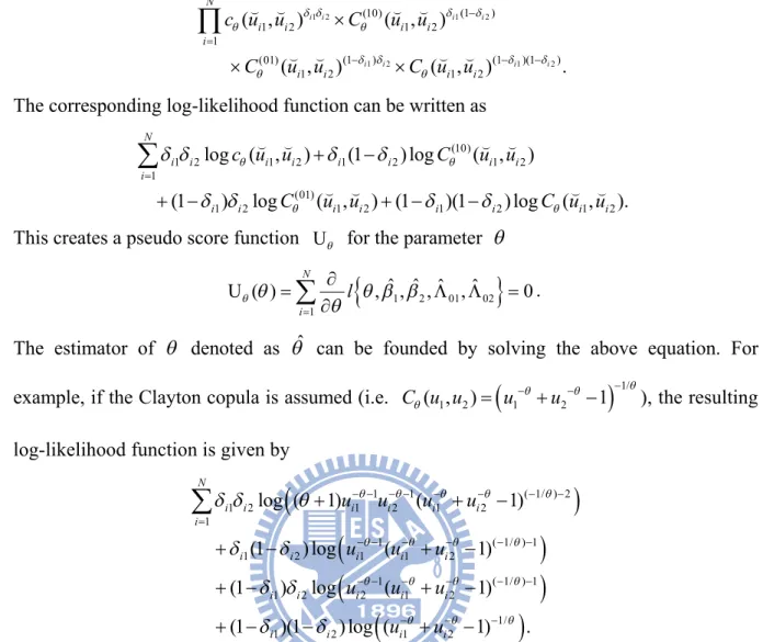
 . In summary, the likelihood function can be written as

1 2 (10) 1(1 2) (01) (1 1) 2 (1 1)(1 2) 1 2 1 2 1 2 1 2 1 ( , ) i i ( , ) i i ( , ) i i ( , ) i i N i i i i i i i i i c u u_   C_ u u   C_ u u   C u u_      



        , where u_{ij 0} ( )exp( jZj) j j S t  

 is a function of  . The corresponding log-likelihood function _j

can be written as (10) 1 2 1 2 1 2 1 2 1 (01) 1 2 1 2 1 2 1 2 log ( , ) (1 ) log ( , ) (1 ) log ( , ) (1 )(1 ) log ( , ). N i i i i i i i i i i i i i i i i i c u u C u u C u u C u u                    



       

Estimation of ( ,  _{1 2}, ) based on the above likelihood function involves the following issues. First u contains the nuisance function _ij S_0j( ) and hence can be not

directly observed. In additional joint estimation of  ( ,  _{1 2}, ) by solving the score equations simultaneous is not an easy task. Shih and Louis (1995)[16] _{proposed a two-stage}

approach. In the first stage, the marginal parameters are estimated. In the second stage, the association parameter  is estimated after plugging in the marginal estimates obtained in

the first stage. This approach was also adopted by Andersen (2005)[3] _{which will be discussed.}

4.3 Marginal Estimation

In this section, we introduce two approaches for marginal estimation.

4.3.1 Likelihood-based approach

The first stage involves estimating pseudo-observations of (U U₁, ₂) which contain the information of the nuisance functions S_0j( ) since under the Cox PH model,

exp( ) 0

( | ) ( ) jZj ( 1, 2)

j j j j j j

U S T Z S T   j . The marginal analysis involves estimating  _j

and S_0j( )t_j . Let t₍₁₎t₍₂₎t_(D) be observed ordered event times and Z_{( )k j} be the jth covariate associated with the individual whose failure time is t_{( )k} , k1, 2,,D. Define the risk set at time t as R( )t { : k T_{( )k} t} which is the set of all individuals who are still under study at a time just prior to t . The regression parameter  can be estimated by _j

maximizing the following partial likelihood

( ) 1 R ( ) exp( ) ( ) ( 1, 2). exp( ) k D j k j j k j lj l t Z L j Z         





Let l(_j)ln_L(_j)_ , then the maximum likelihood estimates can be obtained by

maximizing l(_j). The score equations are solved by taking partial derivatives of l(_j)