行政院國家科學委員會專題研究計畫 成果報告
寬頻合作式無線多輸出入通訊系統--子計畫三:合作式多
輸出入無線通訊之上行傳收器訊號處理技術研究(2/2)
研究成果報告(完整版)
計 畫 類 別 : 整合型
計 畫 編 號 : NSC 99-2219-E-009-010-
執 行 期 間 : 99 年 08 月 01 日至 100 年 07 月 31 日
執 行 單 位 : 國立交通大學電子工程學系及電子研究所
計 畫 主 持 人 : 林大衛
計畫參與人員: 碩士班研究生-兼任助理人員:柯俊言
碩士班研究生-兼任助理人員:張智凱
碩士班研究生-兼任助理人員:陳威宇
碩士班研究生-兼任助理人員:詹曉盈
碩士班研究生-兼任助理人員:余卓翰
碩士班研究生-兼任助理人員:李政憲
碩士班研究生-兼任助理人員:尤基峰
碩士班研究生-兼任助理人員:強丹
博士班研究生-兼任助理人員:王海薇
博士班研究生-兼任助理人員:王柏森
報 告 附 件 : 出席國際會議研究心得報告及發表論文
處 理 方 式 : 本計畫涉及專利或其他智慧財產權,2 年後可公開查詢
中 華 民 國 100 年 10 月 14 日
行政院國家科學委員會補助專題研究計畫成果報告
合作式多輸出入無線通訊之上行傳收器訊號處理技術研究
合作式多輸出入無線通訊之上行傳收器訊號處理技術研究
合作式多輸出入無線通訊之上行傳收器訊號處理技術研究
合作式多輸出入無線通訊之上行傳收器訊號處理技術研究(2/2)
Uplink Transceiver Signal Processing Technology for Cooperative MIMO Wireless
Communication (2/2)
計畫編號:NSC 99-2219-E-009-010
執行期限:99 年 8 月 1 日至 100 年 7 月 31 日
主持人:林大衛 交通大學電子工程學系 教授
計畫參與人員:王海薇、王柏森、柯俊言、張智凱、余卓翰、陳威宇、詹曉盈
李政憲、尤基峰、Chandan Jha 交通大學電子工程學系 研究生
摘要
摘要
摘要
摘要
本計畫為一整合型計畫之子計畫,研究無線通訊之傳輸訊號處理技術。研究內容分
為兩大部份:一為演算法研究,一為數位訊號處理器(DSP)軟體實現研究。其中的研究
子題含:雙向中繼傳輸技術研究、IEEE 802.16m 上行測距技術研究、IEEE 802.16m 多
輸出入傳收技術研究、IEEE 802.16m 初始下行同步技術之數位訊號處理器軟體實現、
以及 IEEE 802.16m 通道估計技術之數位訊號處理器軟體實現。以上前三子題屬演算法
研究,後二子題則係數位訊號處理器軟體實現之研究。
在中繼技術方面,我們探討了一種雙向中繼傳輸方法,等效於可以讓較弱的傳送端
分享較強之傳送端的傳輸功率。在 IEEE 802.16m 上行測距技術方面,我們研究了其相
關規格、演算法與效能。在 IEEE 802.16m 多輸出入傳收技術方面,我們亦研究了其相
關規格、演算法與效能。在 IEEE 802.16m 初始下行同步技術以及 IEEE 802.16m 通道
估計技術之數位訊號處理器軟體實現方面,則係根據我們過去之演算法研究成果,將
其以定點運算方式實現於數位訊號處理器上,並作程式之優化,以利其執行速度。
關鍵詞
關鍵詞
關鍵詞
關鍵詞:
:
:正交分頻多重進接、正交分頻多工、中繼、測距、多輸出入、同步、通道估
:
計
Abstract
This project is a subproject of an integrated project. Its does research in transmission
signal processing technologies for wireless communication. The research conducted in this
project can be divided broadly into two parts: algorithm research and digital signal
processor (DSP) software implementation research. The topics addressed include
bidirectional relaying techniques, IEEE 802.16 uplink ranging techniques, IEEE 802.16m
multi-input multi-output (MIMO) transmission techniques, DSP software implementation of
IEEE 802.16m initial downlink synchronization technique, and DSP software
implementation of IEEE 802.16m channel estimation technique. Of these topics, the first
three pertain to algorithm research and the last two pertain to DSP software implementation
research.
Concerning relaying techniques, we study a bidirectional relaying method which can,
effectively, let the weaker transmitter share the transmission power of the stronger
transmitter. In IEEE 802.16m uplink ranging techniques, we study the corresponding
specifications, algorithms, and performance. In IEEE 802.16m MIMO transmission
techniques, we also study the corresponding specifications, algorithms, and performance. In
DSP software implementation of IEEE 802.16m initial synchronization technique and IEEE
802.16 channel estimation technique, we base the work on our past algorithm research
results. The DSP implementation employs fixed-point computation and we also conduct
code optimization, both for the benefit of execution speed.
Keywords: Orthogonal Frequency-Division Multiple Access (OFDMA), Orthogonal
Frequency-Division Multiplexing (OFDM), Relay, Ranging, Multi-input Multi-output
(MIMO), Synchronization, Channel Estimation
目錄
目錄
目錄
目錄 Table of Contents
一、計畫與報告簡介... 1
二、雙向中繼技術研究... 3
三、IEEE 802.16m 上行測距技術研究 ... 8
四、IEEE 802.16m 多輸出入傳收技術研究 ... 13
五、IEEE 802.16m 初始下行同步技術之數位訊號處理器軟體實現研究 ... 21
六、IEEE 802.16m 通道估計技術之數位訊號處理器軟體實現研究 ... 37
七、參考文獻... 54
八、計畫成果自評... 55
一
一
一
一、
、
、計畫
、
計畫
計畫與報告
計畫
與報告
與報告
與報告簡介
簡介
簡介
簡介
無線通訊技術本就不斷發展,但自從國際電信聯盟射頻通訊標準部門(ITU-R)於幾
年前公布其制定第四代(4G)行動通訊標準 IMT-Advanced 的計畫後,更引發一波相關
的研發浪潮。許多公司與機構都意圖在此一標準中取得一席之地。但由於行動通訊系
統高度複雜,所以這些公司與機構係透過組成團隊的方式來參與 IMT-Advanced 標準
研發。此其中兩個主要的標準團隊就是 IEEE 802.16m 工作團(task group)和第三代行動
通訊夥伴計畫(3GPP)先進長程發展(LTE-Advanced)團體。以空氣介面系統而言,幾個
主要且被這些團隊所積極發展的技術包括:各型多輸出入(multi-input multi-output,
MIMO)傳輸技術、極微細胞(femtocell)系統技術、以及中繼(relay)系統技術。其中底層
的調變方式皆基於正交分頻多工(orthogonal frequency-division multiplexing, OFDM)型
式的技術,含正交分頻多重進接(orthogonal frequency-division multiple access, OFDMA)
和單載波分頻多重進接(single-carrier frequency-division multiple access, SC-FDMA)。
本計畫為一整合型計畫之子計畫,旨在研究無線通訊之傳輸訊號處理技術。其細部
研究內容的規劃,係本於一個思維,即:立足近期標準相關之技術,放眼未來可能之
發展。說明如下。先參 Fig. 1-1,其中所示係根據目前技術發展趨勢,所設想未來無線
傳輸系統之可能環境架構。圖中 BS、RS、與 MS 之間的雙箭頭連線表示無線通道。
實際上,視 BS、RS、與 MS 的相對位置,MS 也可以不經 RS 而直接連上 BS(這也就
是目前行動通訊系統的一般架構,是故此示意圖可說亦涵蓋目前的行動通訊系統架
構)。但一方面這樣的情況比圖中所示者單純,二方面若也顯示直接連接的情況,會使
示意圖太複雜。所以我們只顯示 MS 經 RS 連上 BS 的情況。此系統最複雜的運作情境,
是各 BS、各 RS、和各 MS 都可以有多支天線,而多個 BS 可以同時向多個 RS 傳送訊
號(即 downlink multiuser MIMO 加上 downlink coordinated multi-point [CoMP])或同時接
收從多個 RS 傳來的訊號(即 uplink multiuser MIMO 加上 uplink CoMP),且多個 RS 也
可以同時向多個 MS 同時傳送訊號或同時接收從多個 MS 傳來的訊號。若是 RS 具有
雙向傳收功能(即 bidirectional RS 或 two-way RS),則各 BS 和各 MS 又可以同時向各
RS 傳送訊號,而各 RS 也可以同時向各 BS 和各 MS 傳送訊號。然而以上最複雜的運
作情境,在目前只是一個長程的研究方向,預期還要不少年以後才會趨於實用。較短
期內可以實用化的運作情境,應該比此最複雜的情境要簡單。
Fig. 1-1. 傳輸環境架構示意圖,其中 BS = base station, RS = relay station, MS = mobile
station。
上述具有雙向傳收功能的中繼技術,是最近幾年的新發展,其中有許多可以研發的
課題。在本計畫中我們做了些探討。我們發現一項有趣的中繼訊號處理方式,可以讓
較弱的傳送端虛擬分享較強的傳送端的傳輸功率。這類技術可說還在初起階段,尚未
成為國際標準組織所討論的技術。
在標準相關技術方面,基於過去我們自己在 IEEE 802.16/WiMAX 方面的研究成
果,以及近幾年我國在 WiMAX 和後續 IEEE 802.16m/Advanced WiMAX 標準制定方
面的大力投入,本計畫以 IEEE 802.16m 為基礎進行研究。其研究內容可分兩大部份:
一是演算法研究,一是數位訊號處理器(DSP)軟體實現研究。在演算法方面,本計畫探
討了 IEEE 802.16m 的上行測距技術和多輸出入傳收技術,其中我們研究了 IEEE
802.16m 相關於測距和多輸出入傳收的規格,設計了相關演算法,並以計算機模擬語
數學分析研究其效能。在數位訊號處理器軟體實現研究方面,我們則進行了 IEEE
802.16m 初始下行同步技術和通道估計技術之數位訊號處理器軟體實現。這些實現係
根據我們之前的演算法研究成果,將其以定點運算方式實現於數位訊號處理器上,並
作程式之優化,以利其執行速度。
本計畫為一個二年期計畫的第二年,本報告旨在說明第二年計畫之成果。但在此我
們且用一小段的篇幅,概述兩年的整體研究方向與技術性成果。整體而言,本計畫較
側重上行傳收技術,但亦進行一些下行傳收技術的研究。第一年的研究與成果包括寬
頻無線通道模型之探討、峰均功率比(peak-to-average power ratio, PAPR)控制技術研
究、分散式中繼網路之功率分配技術研究、及載波間干擾(intercarrier interference, ICI)
抑制技術研究等。此外亦開始進行雙向中繼技術研究與上行測距技術研究。第二年(本
年)的研究與成果則如前述,包括雙向中繼技術研究、上行測距技術研究、多輸出入傳
收技術研究、初始下行同步技術之數位訊號處理器軟體實現研究、及通道估計技術之
數位訊號處理器軟體實現研究等。
以下我們分節討論本年度在各技術課題上的研究。第二節討論雙向中繼技術。第三
節討論 IEEE 802.16m 上行測距技術。第四節討論 IEEE 802.16m 多輸出入傳收技術。
第五節討論 IEEE 802.16m 初始下行同步技術之數位訊號處理器實現。第六節討論 IEEE
802.16m 通道估計技術之數位訊號處理器實現。為行文方便,第二節至第六節主要使
用英文。第七節為本報告之參考文獻。第八節為計畫成果自評。
二
二
二
二、
、
、雙向中繼技術
、
雙向中繼技術
雙向中繼技術研究
雙向中繼技術
研究
研究
研究
本節主要內容自下頁起,以學術論文初稿方式呈現。我們將在未來繼續進行相關研
究。
Virtual Sharing of Signal Power via
Fold-and-Forward Two-Way Relaying
Preliminary Draft
Abstract—We consider a two-way relay system where the two
terminal nodes may transmit signals to the relay simultaneously. The relay “folds” the received sum signal and broadcasts the result to both terminals for detection. We show that, with asymmetric channel conditions between the two terminal-relay links, the above operation can tip the error performance between the two directions of transmission in a way that can be viewed as effecting virtual sharing of the transmitter power of the better-conditioned terminal by the worse-better-conditioned. This property also has implication in transmission between terminals that are subject to unequal power constraints.
Index Terms—Amplify-and-forward, physical-layer network
coding, two-way relay.
I. INTRODUCTION
There is much recent interest in applying the concept of network coding to relay-assisted wireless communication. Such coding permits simultaneous reception or transmission of multiple signals at the relay, thereby significantly enhancing the bandwidth efficiency. Some overviews can be found in [1], [2]. One typical structure of such systems is illustrated in Fig. 1, where two terminal nodes T0 and T1 (which have no direct link between them) send signals to each other via the help of the relay node R.
Various network coding methods have been proposed for two-way relaying, some operating in the digital signal domain and requiring the relay to perform some sort of demodulation and some operating in the analog signal domain. Of the latter kind, the simplest merely asks the relay to amplify and broadcast the received sum signal [1]–[4]. Each terminal node can then retrieve the signal destined to it by subtracting a copy of its own transmitted signal from the received broadcast signal, an operation to some extent resembling decision-feedback equalization. While being referred to as a kind of physical network coding, this simple amplify-and-forward (AF) approach deviates from the original XOR network coding [1], [2], [5], [6] in one key aspect. That is, the XOR operation in the original network coding keeps the alphabet size binary whereas AF may double the peak signal amplitude (equivalent to doubling the alphabet size in some sense); the latter could mean 3 dB loss in power efficiency [2]. Note that it is the modulo addition nature of XOR that keeps the alphabet size in the original network coding from expansion. However, to generalize this modulo concept to nonbinary modulations
This work was supported by the Wireless Broadband Communications Technology and Application Project of the Institute for Information Industry which was subsidized by the Ministry of Economic Affairs of the Republic of China as well as by the National Science Council of R.O.C. under Grant NSC 99-2219-E-009-010. 0 0 1 1 R R y =h x+h x+n 1 h h2 0 x x1 ( ) R R x =f y 0 0R 0 y =h x +n y1=h x1R+n1
Fig. 1. System structure, where signal transmission between terminal nodes T1 and T2 is carried out in two phases.
and arbitrary channel conditions is highly nonstraightforward. Some studies in related veins are [7]–[10].
A recent work [11] proposes to have the relay forward the absolute value of its received signal after suitable level-shifting and scaling. It is shown that under fixed channels, this can improve the overall error performance. Since taking the absolute value of a signal can be viewed as a way of “folding” the range of possible signal values (which is also what a modulo operation does), we term the technique fold-and-forward (FF) to allow for later generalization. In this letter, we shed new lights on the analysis and design of this relaying technique. In one aspect, we show that, in two-way relaying, FF can tip the error performance in the two directions of transmission in a way that can be viewed as effecting virtual sharing of the transmitter power of the better conditioned terminal by the worse conditioned. This property can have interesting implications when the two terminals are subject to unequal power constraints or asymmetric channel conditions, such as that between a base station and a mobile station.
In what follows, Sec. II introduces the system model. Sec. III discusses the case where both terminals transmit binary signals. Sec. IV considers the case of higher-order modulations. And Sec. V is the conclusion.
II. SYSTEMMODEL
Consider the two-way relay system shown in Fig. 1, where xi (i = 0, 1) is the signal transmitted by Ti, hiis the channel coefficient between Ti and R, and ni is the additive receiver noise at Ti. In the multiple access (MA) phase the relay receives the signal
yR= h0x0+ h1x1+ nR (1)
where nR is the additive noise at the relay. We assume that both channel coefficients are known to all three nodes.
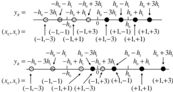
While the system can handle complex signals and complex channel coefficients, due to space limit we only treat the case of real xiand hihere. Hence let xibe an Mi-PAM signal with
0 1 h+h 0 1 h −h 0 1 h h − + 0 1 h h − − 0 R y = −g hF 1 g hF1 0 0 1 ( , )x x = ( 1, 1)− − ( 1, 1)− + ( 1, 1)+ − ( 1, 1)+ + R x = 0 1 ( , )x x =( 1, 1)( 1, 1)+ −− + ( 1, 1)( 1, 1)+ +− − 0 h 0 h −
Fig. 2. Noiseless received and transmitted relay signal constellations for (2,2)-PAM and the corresponding source signal pairs.
modulation as (M0, M1)-PAM. Without loss of generality,
assume h0≥ h1> 0. And define h = h1/h0. In the broadcast
(BC) phase, relay R broadcasts the folded signal xR= f (yR) to T0 and T1. The folding operation and the detection methods at the terminal nodes are described further later.
III. CASE WITH(2,2)-PAM
In the (2,2)-PAM case, we have x0, x1 ∈ {+1, −1}. In
absence of relay noise, the yR constellation consists of either 3 or 4 points, depending on whether h = 1 or h < 1. We concentrate on the latter condition as the former can be considered an asymptotic case of it. The four noiseless received signal points at the relay are given by±h0± h1. Let
the FF operation be given by (similar to [11])
f (yR) = gF(|yR| − h0) (2)
where gF is a scaling factor to satisfy any transmission power constraint of the relay and the subtraction of h0 is to make
xR approximately zero-mean. The exact relation between gF and the relay transmission power will be given later.
The noiseless constellations of yR and xR are illustrated in Fig. 2, together with the corresponding source signal pairs (x0, x1). The constellation for xRsatisfies the “exclusive law” [8], [9]; that is, given x0 (resp. x1), different values of x1
(resp. x0) are mapped to different constellation points. Hence
both terminals can determine the other party’s transmission unambiguously from the received BC signal of the relay, if there is no noise. The detection method (in noise) at terminal Ti (i = 0, 1) is given by ˆ x¯i= { sgn(yi), if xi> 0, −sgn(yi), otherwise, (3) where ˆx¯i is the detected signal at Ti, with ¯0 = 1 and ¯1 = 0, and sgn(·) is the signum function with sgn(0) , 1.
A. Error Performance
For simplicity, assume that n0, n1, and nRare white Gaus-sian (AWGN) with equal variance σ2
n. Because the received signal at either terminal contains two AWGN components, it turns out that the effective decision boundaries and er-ror regions for Ti can be conveniently depicted in a two-dimensional plot as shown in Fig. 3, where the four black dots indicate the noiseless received signal constellation at the relay. In the figure, region I (shaded) applies to the error of having ˆx¯i =−xi when x¯i= xi, and region II that of having ˆ
x¯i = xi when x¯i=−xi. (The decision boundary is the same for all four signal points.) In contrast, the effective decision boundaries under plain AF are as shown in Fig. 4, where gA is the relay amplification factor under AF. For either T0 or T1, the thick solid line (resp. dashed line) indicates the boundary
R y 0 F i g h h i n 0 h 0 h −
Fig. 3. Effective decision boundaries and error regions for (2,2)-PAM under FF for terminal Ti, i = 0, 1.
R y 2 0 A g h 0 n R y 2 1 A g h 1 n 2 0 A g h − 2 1 A g h − 0 h − 1 h − 0 h 1 h
Fig. 4. Effective decision boundaries for (2,2)-PAM under AF at terminals T0 (left) and T1 (right).
when the local transmitter emitted a +1 (resp. −1) in the MA phase. For clarity, signal points associated with the solid-line boundaries are indicated using solid dots, whereas those associated with the dashed-line boundaries are indicated using cross-hatched dots.
The qualitative difference in performance between FF and AF can be gleaned without going to detailed mathematics by comparing Figs. 3 and 4. For this, note that, in high signal-to-noise ratio (SNR), the error probability of each signal point is primarily determined by its distance to the nearest decision boundary. For the sake of argument, let gF = gA for now. Then, by comparing Fig. 3 with the left plot in Fig. 4, we see that the detection error probabilities at T0 (for signals transmitted from T1) under both forwarding schemes are similar. But they are different at T1 (compare Fig. 3 with the right plot in Fig. 4), with AF claiming advantage over FF because the former has a larger distance between each signal point and its associated decision boundary. However, if the relay is power-limited rather than gain-limited, then we can have gF > gA because FF has a smaller relay signal constellation than AF (see Fig. 2). Then the relative performance of FF with respect to AF improves. In particular, FF yields a better performance than AF at T0 by effecting a larger distance between each signal point and its corresponding decision boundary. At T1, the relative performance of FF also improves, but in many conditions (details omitted) still lags that of AF. Compared to AF, therefore, FF may be viewed in some sense as virtually robbing the detection performance of T0 signals (which are detected at T1) in favor of T1 signals (which are detected at T0). Thus the title of this letter.
Employing the formulation proposed in [12], we obtain the bit error rate (BER) under FF at Ti (for signals from T¯i) as
PiF =1 2(P I i + P II i ) (4) with PiI = 1 2π ∫ π−(ϕIi−ϕi) 0 e−2 sin2 θγi(h1)dθ − 1 2π ∫ π−(ϕI i+ϕi) 0 e−γi(2h0+h1)2 sin2 θ dθ (5)
and PiII = 1 2π ∫ π−(ϕi−ϕIIi ) 0 e−2 sin2 θγi(h1)dθ + 1 2π ∫ π−(ϕi+ϕIIi ) 0 e−γi(2h0−h1)2 sin2 θ dθ, (6)
where PiI and PiII stand for, respectively, probability of declaring x¯i = −xi when x¯i = xi and that of declaring x¯i = xi when x¯i=−xi, and γi(z) = z2(gFhi)2 [1 + (gFhi)2]σ2n , ϕi = arctan 1 gFhi , (7) ϕIi = arctanh0+ h1 gFhih0 , ϕIIi = arctanh0− h1 gFhih0 . (8)
From the geometry shown in Fig. 3, we can also see that, in high SNR, PiF ≈ Q ( h1(gFhi) √ 1 + (gFhi)2σn ) (9)
where Q(·) is the Gaussian Q function. In any case, PiF is upper-bounded by two times the Q function value above. On the other hand, the BER at Ti under AF is given by
PiA= Q ( h¯i(gAhi) √ 1 + (gAhi)2σn ) . (10)
Comparing (9) with (10), we see that at T0, it may only take a slightly greater gF than gA to make FF perform better than AF. At T1, some algebra will show that, depending on the relation among h0, h1, and gA, it may or may not be possible to make FF perform better than AF. As to the exact values of gA and gF, suppose the relay is subject to a transmission power constraint PR. Then the maximum allowed gains are given by, respectively,
gA=
√
PR/E[y2R], gF =
√
PR/E[(|yR| − h0)2]. (11)
With some algebra, it can be shown that
E[y2R] = h20+ h21+ σ2n, (12) E[(|yR| − h0)2] = h21+ σn2+ 2h0 [ (h0+ h1)Q ( h0+ h1 σn ) +(h0− h1)Q ( h0− h1 σn )] −h0σn √ 2 π [ e− (h0+h1)2 2σ2n + e− (h0−h1)2 2σ2n ] . (13)
As a numerical example, consider a case where h0 = 1,
h1 = 0.5, and PR = 1. Fig. 5 shows the BER performance. Theory and simulation results agree well. And the results show clearly that, in comparison to AF, FF significantly raises the detection performance of T1 signals (detected at T0) at the expense of the detection performance of T0 signals (detected at T1). Averaged over the two, FF performs slightly better than AF towards the higher-SNR end, in this example.
0 5 10 15 20 10−6 10−5 10−4 10−3 10−2 10−1 100 Nominal SNR (10 log10(1/σn2), dB) BER FF simul., T0 signal FF theory, T0 signal AF simul., T0 signal AF theory, T0 signal FF simul., T1 signal FF theory, T1 signal AF simul., T1 signal AF theory, T1 signal FF simul., average FF theory, average AF simul., average AF theory, average
Fig. 5. BER performance with (2,2)-PAM in AWGN at h0= 1, h1= 0.5,
and PR= 1. 0 31 h+ h 0 1 h−h 0 31 h h − + 0 1 h h − − R y = 0 1 ( , )x x = ( 1, 1)− − ( 1, 3)− + ( 1, 1)+ − 0 ( 1, 3)+ + h 0 h − 0 1 h+h 0 31 h− h 0 31 h h − − − +h0 h1 ( 1, 1)+ + ( 1, 3)+ − ( 1, 3)− − ( 1, 1)− + 0 31 h + h 0 1 h−h 0 31 h h − + 0 1 h h − − R y = 0 1 ( , )x x = ( 1, 1)− − ( 1, 3)− + ( 1, 1)+ −0 ( 1, 3)+ + h 0 h − 0 1 h+h 0 31 h − h 0 31 h h − − − +h0 h1 ( 1, 1)+ + ( 1, 3)+ − ( 1, 3)− − ( 1, 1)− +
Fig. 6. Two kinds of noiseless relay received signal constellation under (2,4)-PAM. Top: separable; bottom: interwoven.
IV. CASE WITHHIGHER-ORDERMODULATIONS
With higher-order modulations, we need to distinguish be-tween two conditions regarding the noiseless received signal constellation at the relay: separable and interwoven. To see what they are, note that, under (M0, M1)-PAM, this noiseless
constellation is a “product constellation” of M0M1 points.
(The points may not be all distinct.) The product constellation may be divided into M0 subconstellations, each associated
with a possible T0 signal value, or M1 subconstellations,
each associated with a possible T1 signal value. Each of the above M0 (resp. M1) subconstellations contains signal
values in the range Rk(0) = [kh0 − (M1 − 1)h1, kh0 +
(M1− 1)h1] (resp. R
(1)
k = [kh1− (M0− 1)h0, kh1+ (M0− 1)h0]), where k ∈ {±1, ±3, . . . , ±(M0 − 1)} (resp. k ∈
{±1, ±3, . . . , ±(M1− 1)}). The separable case refers to the
situation where either any two such R(0)k have at most one point in common or any two such R(1)k have at most one point in common. (Such common points, if any, are end points of some ranges.) Otherwise, the constellation is interwoven. Fig. 6 illustrates the two conditions for (2,4)-PAM with h < 1. For clarity, we distinguish the two M0 subconstellations in
each condition using solid dots and cross-hatched dots. To address the interwoven condition would take much space. Hence we only treat the separable case, which amounts to assuming that h ≤ 1/(M1− 1). In this case, we can fold
R y 0 F i g h h i n 0 h 0 h − 0 21 h− h 0 21 h h − + h0+2h1 0 21 h h − − 0 1 ( 2 ) F i g h h + h 0 1 ( 2 ) F i g h h − h
Fig. 7. Effective decision boundaries for (2,4)-PAM under FF at terminals T1 (thick dashed line) and T0 (all three thick solid and dashed lines).
satisfying the exclusive law so that colocated points are asso-ciated with uniquely distinguishable signals at the terminals [8], [9]. In fact, more than one workable folding method can be conceived. Space precludes a detailed discussion. However, for (2, M1)-PAM the method in (2) suffices. And the
noiseless transmitted signal constellation of the relay is given
by {kgFh1|k = ±1, ±3, . . . , ... ± (M1− 1)}. The detection
method at T1 can be the same as in (3) and that at T0 can be ˆ x1= { min(−3, max(3, ˆxa 1)), if x0> 0, min(−3, max(3, −ˆxa 1)), otherwise, (14) where ˆ xa1= 2· ⌈y1/(2gFh21)⌉ − 1, (15)
with⌈ ⌉ being the ceiling function.
To illustrate the resulting performance, consider (2,4)-PAM with the FF operation as given in (2). Then the effective decision boundaries under FF are as shown in Fig. 7. Hence, in high SNR, the symbol error rate (SER) at Ti (i = 0, 1) (for signals from T¯i) under FF is approximately given by
PiF = KiFQ ( h1(gFhi) √ 1 + (gFhi)2σn ) (16) where K0F = 1.5 and K1F = 0.5. In contrast, that under AF
is approximately given by PiA= KiAQ ( h¯i(gAhi) √ 1 + (gAhi)2σn ) (17) where KA
0 = 1.5 and K1A= 1. We omit detailed derivation as
well as the expressions for the exact SER due to their length. Nevertheless, we note that, for i = 1, the equality in (17) is exact because T0 signals are binary.
Fig. 8 shows the SER performance for the condition h0= 1,
h1= 0.33, and PR= 1. Again, theory and simulation results agree well. And, in comparison to AF, FF again improves significantly the detection performance of T1 signals (detected at T0) at the expense of the detection performance of T0 signals (detected at T1), as discussed.
V. CONCLUSION
We studied the FF technique for two-way relaying. We showed that, in asymmetric channel conditions, FF could tip the error performance in a way that appeared like letting the worse-conditioned terminal share the transmitter power of the better-conditioned terminal virtually. Similar can be said for the case where the two terminals are subject to unequal transmitter power constraints.
5 10 15 20 25 10−6 10−5 10−4 10−3 10−2 10−1 100 Nominal SNR (10 log10(1/σn2), dB) SER FF simul., T0 signal
FF theory, T0 signal FF approx., T0 signal AF simul., T0 signal AF theory, T0 signal FF simul., T1 signal FF theory, T1 signal FF approx., T1 signal AF simul., T1 signal AF approx., T1 signal
Fig. 8. SER performance with (2,4)-PAM in AWGN at h0= 1, h1= 0.33,
and PR= 1. Curves marked “theory” give exact theoretical values, although
their expressions under FF are omitted in this letter.
REFERENCES
[1] K. M. Josiam, Y.-H. Nam, and F. Khan, “Intelligent coding in relays,”
IEEE Veh. Tech. Mag., vol. 4, no. 1, pp. 27–33, Mar. 2009.
[2] F. Rosetto and M. Zorzi, “Mixing network coding and cooperation for reliable wireless communications,” IEEE Wirel. Commun., vol. 18, no. 1, pp. 15–21, Feb. 2011.
[3] S. Zhang, S. C. Liew, and P. P. Lam, “Hot topic: physical-layer network coding,” in Proc. 12th Annual Int. Conf. Mobile Comput. Network. ACM, 2006, pp. 358–365.
[4] P. Popovski and H. Yomo, “Physical network coding in two-way wireless relay channels,” in IEEE Int. Conf. Commun., 2007, pp. 707–712. [5] R. Ahlswede, N. Cai, S.-Y. R. Li, and R. W. Yeung, “Network
informa-tion flow,” IEEE Trans. Inf. Theory, vol. 46, no. 4, pp. 1204-1216, July 2000.
[6] S. Katti, H. Rahul, W. Hu, D. Katabi, M. M´edard, and J. Crowcroft, “XORs in the air: practical wireless network coding,” IEEE/ACM Trans.
Network., vol. 16, no. 3, pp. 497–501, June 2008.
[7] I.-J. Baik and S.-Y. Chung, “Network coding for two-way relay channels using lattices,” in IEEE Int. Conf. Commun., 2008, pp. 3898–3902. [8] T. Koike-Akino, P. Popovski, and V. Tarokh, “Optimized constellations
for two-way wireless relaying with physical network coding,” IEEE J.
Sel. Areas Commun., vol. 27, no. 5, pp. 773–787, June 2009.
[9] T. Uricar and J. Sykora, “Design criteria for hierarchical exclusive code with parameter-invariant decision regions for wireless 2-way relay channel,” EURASIP J. Wirel. Commun. Network., vol. 2010, pp. 1–13, Jan. 2010.
[10] W. Chen, L. Hanzo, and Z. Cao, “Network coded modulation for two-way relaying,” in Proc. IEEE Wirel. Commun. Netowrk. Conf., 2011, pp. 1765–1770.
[11] T. Cui, T. Ho, and J. Kliewer, “Memoryless relay strategies for two-way relay channels,” IEEE Trans. Commun., vol. 57, nos. 10, pp. 3132–3143, Oct. 2009.
[12] J. W. Craig, “A new simple and exact result for calculating the probabil-ity of error for two-dimensional signal constellations,” in IEEE Military
三
三
三
三、
、
、IEEE 802.16m 上行測距技術
、
上行測距技術
上行測距技術研究
上行測距技術
研究
研究
研究
本節主要內容自下頁起,以學術論文初稿方式呈現。這些結果預定將包括在一篇尚
未完成的碩士論文中。
Study in Initial Ranging for IEEE 802.16m
Preliminary Draft
Abstract—We consider the uplink ranging specifications in
IEEE 802.16m and we study the associated uplink ranging method. Simulations are conducted to evaluate the detection performance.
I. INTRODUCTION
Initial ranging is the procedure where a mobile station (MS) expresses desire to connect to a base station (BS). This procedure is variously named in different systems. Whereas it is termed initial ranging in IEEE 802.16m, such a procedure is termed random access in the 3GPP cellular communication systems.
During initial ranging, an MS transmits a ranging signal according to the format and the opportunity provided by the BS. However, due to motion and other reasons, it is likely that the signal arrives at the BS with a time offset, a frequency offset, or a power offset that is outside the allowed range of operation. Upon detection of a ranging signal, the BS may have to initiate a procedure for communicating with the ranging MS to adjust these parameters and to acquire further identity information regarding the MS.
The present study is concerned with the detection of initial ranging signals. In what follows, Sec. II introduces the ranging signal specifications of IEEE 802.16m. Sec. III presents the proposed ranging signal detection method which also obtains the timing of the detected signal. It will also present some simulation results. Sec. IV considers carrier frequency offset (CFO) estimation following detection of the ranging signals. And Sec. V is the conclusion.
II. RANGINGSIGNAL INIEEE 802.16M
The ranging channel in IEEE 802.16m can be classified into ranging channel for synchronized and non-synchronized MSs, where the former is for so-called “periodic ranging” and the latter is for initial access and handover. We consider the latter only.
According to IEEE 802.16m, a physical ranging channel for non-synchronized MSs consists of the ranging preamble (RP) with length of TRP depending on the ranging subcarrier spac-ing△fRP, and the ranging cyclic prefix (RCP) with length of TRCP in the time domain, where TRP,△fRP, and TRCP are some parameters. A ranging channel occupies a bandwidth of one subband. The ranging channel has two formats as described in Table I, where Tb, Tg, and △f are some other paramters, k1= (Nsym+ 1)/2 and k2= (Nsym− 4)/2, with Nsym being the number of OFDMA symbols in a so-called “advanced air interface” (AAI) subframe. In our work, for simplicity, we let Tb = 1024, Tg= 128,△f = 10.9375 kHz, and Nsym= 6, which are a proper set of values under IEEE 802.16m.
TABLE I
RANGINGCHANNELFORMATS ANDPARAMETERS Format No. TRCP TRP △fRP
0 k1× Tg+ k2× Tb 2× Tb △f/2
1 3.5× Tg+ 7× Tb 8× Tb △f/8
Fig. 1. Ranging channel allocation in AAI subframe [1, Fig. 570(a)].
Ranging channel for non-synchronized AMSs is allocated in one or three uplink (UL) AAI subframes for format 0 or format 1, respectively. Format 0 has a repeated structure as shown in Fig. 1. The transmission start time of the ranging channel is aligned with the UL AAI subframe start time at the AMS. The remaining time duration of the AAI subframes is reserved to prevent interference between the adjacent AAI subframes.
For initial ranging, each MS randomly chooses one of the ranging preamble codes from the available set of ranging preamble codes specified by the BS. These codes are Zadoff-Chu sequences. The pth ranging preamble code xp(k) is given by
xp(k) = exp(−j · π ·
rp· k(k + 1) + 2 · k · sp· NCS
NRP
), (1) where NRP, rp, sp, and NCS are some parameters. Based on the IEEE 802.16m specifications, we have NRP = 139. For a detailed definition of the other parameters, we refer to [1].
III. RANGINGSIGNALDETECTION ANDTIMING
ESTIMATION
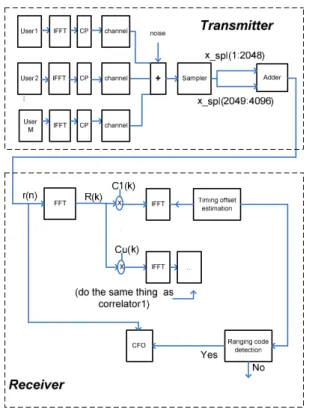
Fig. 2 shows the overall UL transmitter and receiver system. W assume that there may be more than one user transmitting ranging signals at the same time. The receiver at the BS will collect 4096 samples of the received signal located in the middle of a subframe as shown in Fig. 3. We add the first 2048 points to the latter 2048 points together to get r(n). This is because the ranging signal has a two-times repetition structure as shown in Fig. 1. After the timing offset estimation and ranging code detection blocks, the output contains the information of detected codes and estimated timing offsets. Details of these blocks are described below.
We assume that the BS allocates u possible ranging codes, where u = 8. So the BS has to correlate each of these codes with R(k) to determine if any of them is present and, for each
…
Fig. 2. Uplink transmitter and receiver system.
Fig. 3. Typical locations of received ranging signals in a subframe and the location of the 4096 samples taken by the BS receiver.
code that is present, its timing. This correlation is performed in the frequency domain for equivalent performance with a reduced complexity than time-domain correlation [2]. In this, we first perform 2048-point FFT on r(n) to get R(k). It is then multiplied point-wise with each of the u possible frequency-domain sequences Ci(k) (i = 1, 2, . . . , u) constructed from the usable ranging codes. Recall that a ranging code is a 139-sample sequence. Therefore, each 2048-point sequence Ci(k) contains 139 nonzero points that hold one Zadoff-Chu ranging code at the subcarriers specified by the BS for ranging use. The remaining 1909 subcarriers are all zero. Each of the 2048-point product is subject to a 2048-point IFFT. The results after IFFT, denoted Ui(m), consist of 2048 complex values each. In a noiseless and interference-free situation, each Ui(m) for which code i is present would be a bandpassed version of the wireless channel response. Otherwise, it would be null. In noise and interference (particularly that due to nonorthogonality between the ranging codes), the above conditions will not hold. But we can nonetheless use Ui(m) for code and timing detection. Specifically, the norm operation (i.e., taking the absolute value) is performed on each point of Ui(m). The norm values are used for code detection and timing offset estimation.
0 1 2 3 4 5 6 7 8 0 0.1 0.2 0.3 0.4 0.5 0.6 0.7 0.8 0.9 1 threshold value probability
Miss Detection Rate(correlator1) for Simulation and Theory in the AWGN channel theory
simulation
Fig. 4. Simulated miss detection probability in AWGN versus theory.
0 1 2 3 4 5 6 7 8 0 0.1 0.2 0.3 0.4 0.5 0.6 0.7 0.8 0.9 1 threshold value probability
False Alarm Analysis Compared to the Simulaton Results in the AWGN channel theory simulation
Fig. 5. Simulated false alarm probability in AWGN versus theory.
We detect the presence/absence of a code by comparing
|Ui(m)| to a threshold. The threshold has to be chosen
accord-ing to the desired performance in miss detection probability and false alarm probability. The setting of such a desired performance has to do with overall wireless system design and is outside the scope of the present study. Suffice it to say that a higher detection threshold results in a higher miss detection probability but a lower false alarm probability. The contrary holds for a lower detection threshold.
We conducted some analysis on the relation between the detection threshold and the two probabilities based on the assumption that the inter-ranging code interference is Gaus-sian. The detailed analysis is not reproduced here. Figs. 4 and 5 show some simulated results on miss detection probability and false alarm probability in additive white Gaussian noise (AWGN) and compare them with theory. We see that the theoretical results provide a rather conservative prediction of the detection performance due to the Gaussian assumption on interference, which is an inexact model of the actual situation. Nevertheless, the shapes of the theoretical and simulated performance curves are quite similar and they appear to be horizontal translations of each other.
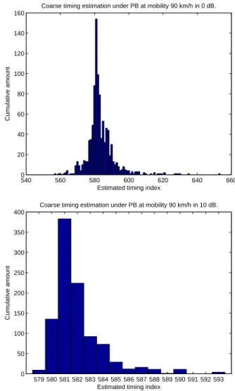
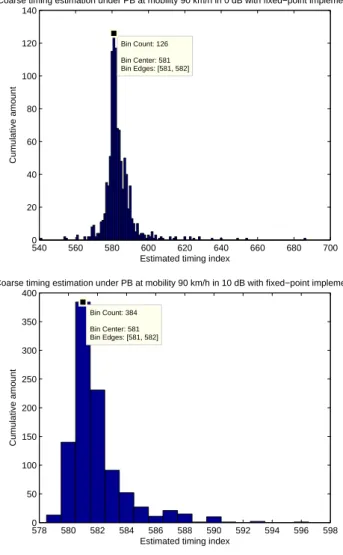
We now turn to look at the performance in timing es-timation of the ranging signals. Figs. 6 and 7 show some simulation results with different number of ranging signals from different users occupying the same ranging channel, with
−200 −15 −10 −5 0 5 10 15 20 0.2 0.4 0.6 0.8 1 1.2 1.4
Average Sample Offset RMSE in the AWGN channel
SNR(dB)
average sample offset RMSE
3 users 2 users 1 user
Fig. 6. Timing estimation accuracy in AWGN with different number of ranging signals occupying the same ranging channel.
−201 −15 −10 −5 0 5 10 15 20 1.1 1.2 1.3 1.4 1.5 1.6 1.7 1.8
Average Sample Offset RMSE in the SUI3 channel
SNR (dB)
average sample offset RMSE
1 user 2 users 3 users
Fig. 7. Timing estimation accuracy in SUI3 channel with different number of ranging signals occupying the same ranging channel.
all users’ wireless channels being AWGN or SUI3 [3]. (The SUI wireless channels were originally developed for fixed wireless access studies. But they have been used for mobile radio studies by imposing a greater Doppler spread on their channel multipaths.) The performance in different wireless channel conditions show similar general trends, although they are different in details. We see that, even with three ranging users in one ranging channel, the root-mean-square (RMS) timing error is still under two sample, which appears accurate enough for practical application.
Now consider a case where there may be one, two, or three users transmitting ranging signals in the same ranging channel, but the multipath wireless channels of the users are different. Fig. 8 shows some results, where TU stands for the 6-path typical urban channel [4, ch. 2]. In this case, the performance is worse than in the previous two cases. But the maximum RMS timing error (which occurs with three users transmitting ranging signals in the same ranging channel) is still under four samples down to approximately −15 dB of signal-to-noise ratio (SNR), which appears sufficiently good for application.
IV. CARRIERFREQUENCYOFFSETESTIMATION
After detection of the ranging signals and estimation of their timing, we proceed to estimate their CFOs. This is so that the BS may feed this information back to the MSs for
−200 −15 −10 −5 0 5 10 15 20 2 4 6 8 10 12 14 16 18
Average Sample Offset RMSE in the hybrid channel (SUI1, SUI3, TU)
SNR (dB)
average sample offset RMSE
1 user 2 users 3 users
Fig. 8. Timing estimation accuracy with different number of ranging signals occupying the same ranging channel. The ranging signals experience different multipath wireless channels.
1 i≠
∑
i Q≠∑
… … … … … … … …Fig. 9. Proposed multiple CFO estimation method.
carrier frequency adjustment. As there may be more than one ranging signals occupying the same ranging channel, we propose an iterative method for CFO estimation based on parallel interference cancellation. The method is illustrated in Fig. 9. It is motivated by [5].
Note that, in the UL, we expect the ranging signals are only subject to fractional CFO (where the CFO normalized to the subcarrier spacing is a fractional number). This is because before the MS attempts ranging, it has to have already executed an initial downlink (DL) synchronization procedure to acquire the ability to receive DL signals from the BS.
In Fig. 9, s(m)i (n) denotes the interference-cancelled version of the ith ranging signal after the mth iteration. In each iteration, the CFO of the ith ranging signal is estimated as
ˆ εi= 1 −2π∠ ∑ n yi(n)· yi∗(n + N ), i = 1, 2, ..., Q, (2) where Q is the number of ranging signals and yi(n) is the interference-cancelled received signal.
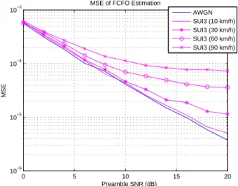
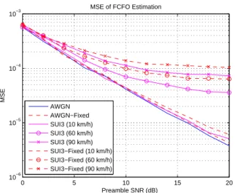
Fig. 10 shows some results of the estimation performance with all ranging signals in AWGN. The MSEs for all three ranging signals (users) decrease linearly with increasing SNR, which appears intuitively reasonable. Fig. 11 shows some results with the ranging signals experiencing different wireless channels. The performance becomes worse than that in AWGN (which may be intuitively expected) and channel-dependent
−20 −18 −16 −14 −12 −10 −8 −6 −4 −2 10−5
10−4 10−3 10−2
Three Users CFO MSE in the AWGN channel
SNR (dB)
Normalized MSE
User 1 User 2 User 3
Fig. 10. MSE of CFO estimation where the ranging signals from different users experience different wireless channels.
−20 −18 −16 −14 −12 −10 −8 −6 −4 −2
10−5 10−4 10−3 10−2
10−1 Three Users CFO MSE in the hybrid channel (SUI3, SUI1, Rayleigh)
SNR (dB)
Normalized MSE
User 1 User 2 User 3
Fig. 11. MSE of CFO estimation in AWGN, where normalization is with respect to subcarrier spacing.
(which may also be intuitively expected). In any case, the MSE can be smaller than 1% of the subcarrier spacing (i.e., its square root being smaller than 10% of the subcarrier spacing) even with a very low SNR.
Concerning the convergence speed of the iterative estima-tion method, simulaestima-tions show that it converges in several iterations. Fig. 12 shows one set of results for a very low SNR (−19 dB). In a higher SNR, the convergence can be even faster.
V. CONCLUSION
We have studied the ranging specifications of IEEE 802.16m. We proposed a ranging signal detection method which can also detect the timing of the received ranging signals. In addition, we proposed a method for estimating the carrier frequency offsets of the received ranging signals. The performance of these methods has been investigated with computer simulation. It was shown that we could still attain a reasonable level of performance even if multiple ranging signals were transmitted in the same ranging channel.
REFERENCES
[1] IEEE P802.16m/D12, Draft Amendment for IEEE Standard for Local
and Metropolitan Area Networks — Part 16: Air Interface for Fixed and Mobile Broadband Wireless Access Systems — Advanced Air Interface.
New York: IEEE, Feb. 2011.
0 5 10 15 20 0.008 0.01 0.012 0.014 0.016 0.018 0.02 0.022 0.024
Convergence Behavior of Users in the hybrid channel (SUI3, SUI1, Rayleigh) (−19dB)
Iteration Times
Normalized MSE
User 1 User 2 User 3
Fig. 12. Convergence behavior of iterative CFO estimation with multiple ranging signals occupying the same ranging channel with the signals experi-encing different wireless channels.
[2] Soon Seng Teo, “IEEE 802.16e OFDMA TDD ranging process and uplink transceiver integration on DSP platform with real-time operating system,” M.S. thesis, Industrial Technology R&D Master Program on Communication Engineering, National Chiao Tung University, Jan. 2008.
[3] V. Erceg et al., “Channel models for fixed wireless applications,” IEEE 802.16.3c-01/29c4, July 2001.
[4] G. L. St¨uber, Principles of Mobile Communication, 2nd ed. Kluwer Academic, 2001.
[5] J. G. Andrews, “Interference cancellation for cellular systems: a con-temporary overview,” IEEE Wireless Commun. Mag., vol. 12, no. 2, pp. 19–29, Apr. 2005.
四
四
四
四、
、
、IEEE 802.16m 多輸出入傳收
、
多輸出入傳收
多輸出入傳收技術
多輸出入傳收
技術
技術
技術研究
研究
研究
研究
Study on Precoding and Equalization for the Spatial
Multiplexing Mode of IEEE 802.16m
Preliminary Draft
Abstract—We focus on precoding and equalization for the
spatial multiplexing mode of IEEE 802.16m closed-loop MIMO. In IEEE 802.16m MIMO systems, the precoding matrix is computed at the receiver, and then fed back to the transmitter. To reduce the fed back datas, only preferred matrix index is fed back. The preferred matrix index is selected from a subset of precoder called codebook defined by IEEE 802.16m. We based on zero-forcing (ZF) and minimum mean square error (MMSE) equalizer to design the selection method to select the best precoder. We proposed MMSE-Based and MaxminSNR-Based method. MMSE-MaxminSNR-Based method finds the precoder has the minimum mean square error. MaxminSNR-Based method finds the precoder that maximizes the minimum SNR of the two antennas. This method has to calculate each precoders antenna SNR. Then, we select the appropriate one to transmit back. We will compare with SVD-based and optimal precoder.
I. INTRODUCTION
Orthogonal frequency division multiple access (OFDMA) has emerged as one of the prime multiple access schemes for broadband wireless networks. Some major examples are IEEE 802.16 Mobile WiMAX, IEEE 802.20 and 3GPP LTE. As a special case of multicarrier multiple access schemes, OFDMA exclusively assigns each subchannel to only one user, eliminat-ing intra-cell interference. In frequency selective channels, an intrinsic advantage of OFDMA is its capability to exploit the so-called multiuser diversity provided by multipath channels. Other advantages of OFDMA include finer granularity and better link budget [12]. OFDMA can be easily generated using an inverse fast Fourier transform (IFFT) and received using a fast Fourier transform (FFT).
The IEEE 802.16 standard committee has developed a group of standards for wireless metropolitan area networks (MANs). OFDMA is used in the 2 to 11 GHz systems. The IEEE Standard 802.16-2004 was for broadband wireless access systems that provide a variety of wireless access services to fixed outdoor and indoor users. The 802.16e was designed to support terminal mobility with a speed up to 120 km/h [15]. The last two standards have now been combined in IEEE 802.16-2009.
In response to International Telecommunication Union Ra-diocommunication Section (ITU-R)’s plan for the fourth-generation mobile communication standard IMT-Advanced, the IEEE 802.16 standards group has set up the 802.16m (i.e., Advanced WiMAX) task group. The new frame structure developed by IEEE 802.16m can be compatible with IEEE 802.16e, reduce communication latency, support relay, and coexist with other radio access techniques (in particular, LTE). In the IEEE 802.16m working group, the high-level system description and evaluation methodology are captured in [9].
MIMO technologies again play an essential role in achieving the ambitious target set, which requires the 802.16m system to deliver twice the performance gain over a baseline 802.16e system in various measures, including sector throughput, av-erage user throughput, and peak data rate, as well as cell-edge performance. Several new MIMO ingredients are proposed. Noticeable ones are transformed codebook for beamforming feedback, differential beamforming feedback, open-loop mul-tiuser MIMO, and collaborative multicell MIMO [13]. We study the MIMO architecture and signal processing technology for 802.16m. In particular, we consider the zero-forcing (ZF) equalizer and minimum mean-square error (MMSE) equalizer approach wherein we employ the technique proposed in [2]. We follow [2] to introduce the ZF and MMSE equalizer with channel feedback selection problem.
This paper focuses on the precoding and equalization for the spatial multiplexing mode of IEEE 802.16m closed-loop (CL) multi-input multi-output (MIMO) systems. A problem associated with precoding is that the channel state information must be known at the transmitter. This may be difficult since the bandwidth of the feedback channel is usually limited. Thus, a codebook-based limited feedback precoding scheme is generally used. The main idea is to quantize the precoding matrix and feedback the index of the optimum precoder. We propose two methods to select the best precoder from a finite set of precoding matrices and we will compare with two other methods.
II. INTRODUCTION TOIEEE 802.16M
We introduce the IEEE 802.16m basic frame structure and MIMO transmission mechanism. Much of the material is taken from [10].
A. Frame Structure
The AAI basic frame structure is illustrated in Fig. 1. Each 20 ms superframe is divided into four 5-ms radio frames. When using the same OFDMA parameters with channel bandwidth of 5, 10, or 20 MHz, each 5-ms radio frame further consists of eight subframes for G = 1/8 and 1/16. There are four types of subframes:
• Type-1 subframe consists of six OFDMA symbols.
• Type-2 subframe consists of seven OFDMA symbols.
• Type-3 subframe consists of five OFDMA symbols.
• Type-4 subframe consists of nine OFDMA symbols.
This type shall be applied only to UL subframe for the 8.75 MHz channel bandwidth when supporting the WirelessMAN-OFDMA frames.
Fig. 1. Basic frame structure for 5, 10 and 20 MHz channel bandwidths (Fig.466 in [10]).
The basic frame structure is applied to FDD and TDD duplexing schemes, including H-FDD MS operation. The number of switching points in each radio frame in TDD systems shall be two, where a switching point is defined as a change of directionality, i.e., from DL to UL or from UL to DL.
B. Downlink MIMO Architecture and Data Processing The architecture of downlink MIMO at the transmitter side is shown in Fig. 2. The MIMO encoder block maps L MIMO layers (L≥ 1) onto MtMIMO streams (Mt≥ L), which are fed to the precoder block. For the spatial multiplexing modes in SU-MIMO, “rank” is defined as the number of MIMO streams to be used for the user allocated to the Resource Unit (RU). For SU-MIMO, only one user is scheduled in one RU, and only one forward error correction (FEC) block exists at the input of the MIMO encoder (vertical MIMO encoding at trans-mit side). For MU-MIMO, multiple users can be scheduled in one RU, and multiple FEC blocks exist at the input of the MIMO encoder (horizontal MIMO encoding or combination of vertical and horizontal MIMO encoding at transmit side, which is called multi-layer encoding). The precoder block maps MIMO stream(s) to antennas by generating the antenna-specific data symbols according to the selected MIMO mode. The subcarrier mapper blocks map antenna-specific data to the OFDM symbol.
Fig. 2. DL MIMO architecture (Fig.537 in [10]).
C. MIMO Layer to MIMO Stream Mapping
MIMO layer to MIMO stream mapping is performed by the MIMO encoder. The MIMO encoder is a batch processor that operates on M input symbols at a time. The input to the MIMO encoder is represented by an M × 1 vector as
s = s1 s2 .. . sM (1)
where siis the ith input symbol within a batch. In MU-MIMO transmissions, the M symbols belong to different AMSs. Two consecutive symbols may belong to a single MIMO layer. One AMS shall have at most one MIMO layer. MIMO layer to MIMO stream mapping of the input symbols is done in the space dimension first. The output of the MIMO encoder is an
Mt× NF MIMO STC matrix as,
x = S(s), (2)
which serves as the input to the precoder, where Mt is the number of MIMO streams, NF is the number of subcarriers occupied, x is the output of the MIMO encoder, s is the input MIMO layer vector, and S() is a function that maps an input MIMO layer vector to an STC matrix which will be further defined specifically for various cases below. There are four MIMO encoder formats (MEF): SFBC, vertical en-coding (VE), multi-layer enen-coding (ME), and conjugate data repetition (CDR). For SU-MIMO transmissions, the STC rate is defined as R = M
NF
For MU-MIMO transmissions, the STC rate per user (R) is equal to 1 or 2.
1) SFBC Encoding: The input to the MIMO encoder is a
2× 1 vector s = [ s1 s2 ] , (3)
and the MIMO encoder generates the 2× 2 SFBC matrix
x = [ s1 −s∗2 s2 s∗1 ] . (4)
Where x is a 2 × 2 matrix The matrix x occupies two
consecutive subcarriers.
2) Vertical Encoding (VE): The input and the output of MIMO encoder are both the same M × 1 vector as
x = s = s1 s2 .. . sM (5)
where si, 1≤ i ≤ M, belong to the same MIMO layer. The encoder is an identity operation.
3) Multi-layer Encoding (ME): The input and the output of MIMO encoder are again the same M× 1 vector
x = s = s1 s2 .. . sM , (6)
Mode index Description MIMO encoding
format (MEF) MIMO precoding
Mode 0 OL SU-MIMO (Tx
diversity) SFBC Non-adaptive
Mode 1 OL SU-MIMO (SM) VE Non-adaptive
Mode 2 CL SU-MIMO (SM) VE Adaptive
Mode 3 OL MU-MIMO (SM) ME Non-adaptive
Mode 4 CL MU-MIMO (SM) ME Adaptive
Mode 5 OL SU-MIMO (Tx
diversity) CDR Non-adaptive
Fig. 3. Downlink MIMO modes (from [10, Table 844]).
but now si, 1 ≤ i ≤ M belong to different MIMO layers, where two consecutive symbols may belong to a single MIMO layer. Multi-layer encoding is only used for MU-MIMO mode. The encoder is an identity operation.
4) Conjugate Data Repetition (CDR) Encoding: The input to the MIMO encoder is a 1× 1 vector
s = s1, (7)
yielding
x = [s1 s∗1], (8)
The CDR matrix x occupies two consecutive subcarriers.
D. Downlink MIMO Modes [10]
There are six MIMO transmission modes for unicast DL MIMO transmission as listed in Fig. 3 and 4. The allowed values of the parameters for each DL MIMO mode are shown in Figure 4.
E. Feedback Mechanisms and Operation [10]
1) MIMO Feedback Mode Selection: An AMS may send an unsolicited event-driven report to indicate its preferred MIMO feedback mode to the ABS. Event-driven reports for MIMO feedback mode selection may be sent on the P-FBCH during any allowed transmission interval for the allocated P-FBCH. The MIMO feedback mode are shown in Fig.5.
III. SYSTEMMODEL
We consider a system as shown in Fig. 6.
Information bits for subcarrier k are first passed through the modulator and sent into the encoder. There are four different types of encoder, but we will not discuss them. After passing through the encoder, there are M streams. Let s be the symbol vector at the encoder output as
sk= [sk,1sk,2. . . sk,M]T. (9)
For convenience, we assume that the M data streams are equally-powered and independent to each other. That is, E[sks∗k] = IM which A∗denotes complex-conjugate of matrix
A. We denote the precoder by F. F is an Nt×M matrix. There are several precoder codebook sets. The signal after precoding can be expressed as xk= Fsk. (10) Number of transmit antennas STC rate per MIMO layer Number of MIMO streams Number of
subcarriers Number of MIMO layers Nt R Mt NF L MIMOmode 0 24 11 22 22 11 8 1 2 2 1 MIMOmode 1 and MIMOmode 2 2 1 1 1 1 2 2 2 1 1 4 1 1 1 1 4 2 2 1 1 4 3 3 1 1 4 4 4 1 1 8 1 1 1 1 8 2 2 1 1 8 3 3 1 1 8 4 4 1 1 8 5 5 1 1 8 6 6 1 1 8 7 7 1 1 8 8 8 1 1 MIMOmode 3 and MIMOmode 4 2 1 2 1 2 4 1 2 1 2 4 1 3 1 3 4 1 4 1 4 8 1 2 1 2 8 1 3 1 3 8 1 4 1 4
Fig. 4. DL MIMO parameters (from [10, Table 845]).
where xk is a length Nt vector and Nt is the number
of transmit antennas. We assume that Nt > M . Then we transform the signal vector to the time domain using IDFT and add CP. Let the number of the receive antenna be Nr. We consider a multipath channel, whose input-output relation in the frequency domain can be written as
yk= HFxk+ nk. (11)
where yk is the received symbol vector, H is the Nt× Nr
channel matrix and nk is the Nr × 1 noise vector. We
assume that the entries of H are independent and identically distributed (i.i.d.) and their distributions are complex normal with zero mean and unit variance, denoted by CN (0, 1). Similarly, the entries of nk are also i.i.d. and the distribution is CN (0, N0). After passing the signal over the channel, we
remove the CP and transform the result back to frequency domain. We consider two different kinds of equalizer, ZF and MMSE. Let G be the M × Nrequalizer matrix.
We set each symbol has the same precoder so the optimum equalizer for the MMSE equalizer is given by
G = (HFFHHH+ Rn)−1HF. (12) On the other hand, the ZF equalizer can be derived as
G = (HF)†. (13)
In either case, the signal vector at the equalizer output is given by
ˆ
MIMO Feedback Mode Description and Type of RU
Feedback Content Support MIMO Mode
Outside the OL region Mode Inside the OL Support MIMO region 0 OL SU MIMO SFBC/SM (Diversity: DLRU, NLRU) Sounding based CL SU and MU MIMO 1. STC rate
2. Wideband CQI MIMO mode 0 and MIMO mode 1 Flexible adaptation between the two modes STC rate=1:SFBC CQI 2<=STC rate<=4:SM CQI In DLRU: Mt=2 for SM
In NLRU: Mt>=2 for SM
For sounding based CL SU MU MIMO, STC rate =1:SFBC CQI
MIMO mode 0 and MIMO mode 1 Flexible adaptation between the two modes STC rate=1:SFBC CQI STC rate=2:SM CQI In DLRU only 1 OL SU MIMO SM (Diversity: NLRU)
1. Wideband CQI n.a MIMO mode 5 STC rate = 1/2 2 OL SU MIMO SM (localized: SLRU) 1. STC rate 2. Subband CQI 3. Subband selection MIMO Mode 1
1<=STC rate<=8 MIMO mode 5STCrate = 1/2
3 CL SU MIMO (localized: SLRU) 1. STC rate 2. Subband CQI 3. Subband PMI 4. Subband selection 5. Wideband correlation matrix MIMO mode 2 1<=STC rate<=8 n.a 4 CL SU MIMO(Diversity: NLRU) 1. Wideband CQI 2. Wideband PMI 3. Wideband correlation matrix MIMO mode 2 (Mt≦4) n.a 5 OL MU MIMO (localized: SLRU) 1. Subband CQI 2. Subband selection 3. MIMO stream indicator
MIMO mode 3 MIMOmode 3
6 CL MU MIMO (localized: SLRU) 1. Subband CQI 2. Subband PMI 3. Subband selection 4. Wideband correlation matrix
MIMO mode 4 n.a
7 CL MU MIMO (Diversity: NLRU) 1. Wideband CQI 2. Wideband PMI 3. Wideband correlation matrix MIMOmode 4 n.a
Fig. 5. MIMO feedback modes (from [10, Table 849]).
Fig. 6. System structure.
IV. PROPOSEDFEEDBACKSELECTIONSCHEMES
In this section, we derive two feedback selection schemes max minSNR-based search method and MMSE-based exhaus-tive search method that can greatly reduce the complexity.
A. MaxminSNR-Based Search Method
In this method, We maximize the minimum SNR at the receiver antennas under MMSE or ZF equalization. It can be thought as minimize the maximum symbol error rate (SER) at the receive antennas. The signal power per receive antenna can be expressed as
| gT
kHFix|2. (15)
The noise power is
σn2 | gkTgk| . (16)
The optimum precoding matrix F selected from the codebook
C maximizes the minimum SNR of at the receive antennas as F = arg max Fi min k|Fi SNRk = arg max Fi min k|Fi | gT kHFix|2 σ2 n | gkTgk| (17)
where k is the index of the receive antennas, i is the index of the precoder, and gk is the equalizer for kth receive antenna.
B. MMSE-Based Exhaustive Search Method
In this method, we minimize the mean square error (MSE) between ˆX and X under the ZF or the MMSE equalizer. We
compare all possible precoders to find the best one in the source that
min M SE = arg min Fi
∥ ˆX− X∥2. (18)
For ZF equalizer, therefore, min M SE = arg min
Fi
∥(HFi)†HFiX + (HFi)†n− X∥ 2
, (19) and for the MMSE equalizer,
min M SE = arg min Fi ∥(HFiFHi H H+ R−1 n )HFiHFiX + (HFiFHi HH+ R−1n )HFin− X∥2. (20) Then we will transmit the precoder index i back to the transmitter. The transmitter will use this precoder to allocate the power. In this method, the computation of complexity is high, because we have to evaluate all the precoders.
V. SIMULATIONRESULTS
In the simulation, we consider both additive white Gaussian noise (AWGN) channels.
A. System Parameter and Channel Model
Channel models for evaluation of IMT-Advanced candidate radio interface technologies [6]. We use the Suburban macro-cell model. The parameter are in Fig. 7. The root-mean-square (RMS) delay spread of Suburban macrocell channel is 75.7485 ns. Table I gives the primitive and derived parameters used in our simulation work. The results are averages over 10,000,000 channel realizations.
B. Two Transmit Antennas and Two Receive Antennas with Rank Two
For comparison, we consider a no feedback system with feedback system.
First, consider the case of AWGN channels. Fig. 8 shows the symbol-error-rate (SER) performance of the systems. There is no difference between theory, MMSE equalizer with feedback and MMSE equalizer without feedback.
TABLE I
OFDMA DOWNLINKPARAMETERS Parameters Values Bandwidth 10 MHz Central frequency 3.5 GHz Nused 865 Sampling factor n 28/25 G 1/8 NF F T 1024 Sampling frequency 11.2 MHz Subcarrier spacing 10.94 kHz Useful symbol time 91.43 µs CP time 11.43 µs OFDMA symbol time 102.86 µs Sampling time 44.65 ns
Cluster
# Delay [ns] Power [dB] AoD [ 。 。 。
。] AoA [。。。。] Ray power [dB] 1 0 5 10 -3.0 -5.2 -7.0 0 0 -13.0 2 25 -7.5 13 -71 -20.5 3 35 -10.5 -15 -84 -23.5 4 35 -3.2 -8 46 -16.2 5 45 50 55 -6.1 -8.3 -10.1 -12 -66 -16.1 6 65 -14.0 -17 -97 -27.0 7 65 -6.4 12 -66 -19.4 8 75 -3.1 -8 -46 -16.1 9 145 -4.6 -10 -56 -17.6 10 160 -80 -13 73 -21.0 11 195 -7.2 12 70 -20.2 12 200 -3.1 8 -46 -16.1 13 205 -9.5 14 -80 -22.5 14 770 -22.4 22 123 -35.4 Cluster ASBS= 2° Cluster ASMS= 10°
Fig. 7. Suburban macrocell channel model [9].
0 2 4 6 8 10 12 10−5 10−4 10−3 10−2 10−1 100 AWGN Channel SNR(dB) SER Theory
MMSE equalizer without feedback MMSE equalizer with feedback
Fig. 8. SER performance in AWGN.
Second, we consider the case of suburban macrocell channel with 2 transmit antennas and 2 receive antennas transmiting two streams. Figs. 9–12 show the performance of different feedback methods at velocities of 30 and 120 km/h. We can see that both MSE and SER have the same curve. This is because the MMSE equalizer is finding the minimum mean square error and it also can be seem worked in SER. The optimum precoder method leads all the methods because it use the sounding method to transmit back the best precoder. Also both ZF and MMSE equalizer can achieve diversity one. We also compare all the methods in ZF and MMSE equalizer. MMSE equalizer leads the ZF equalizer both in MSE and SER. This is because ZF equalizer has the noise enhancement problem. We can see that there is almost no gain with precoding and no precoding. 0 5 10 15 20 25 30 10−2 10−1 100 101 102 103
Different equalizer with different feedback V30
SNR (dB) Normalize MSE ZF,,No feedback ZF, Codewordsearch ZF, MMSE Calculate ZF, MaxminSNR ZF, Optimum Precoder MMSE, No feedback MMSE, Codewordsearch MMSE, MMSE Calculate MMSE, MaxminSNR MMSE, Optimum Precoder
Fig. 9. MSE for QPSK using ZF and MMSE equalizer with different feedback methods at 30 km/h in multipath Suburban channel.
0 5 10 15 20 25 30
10−3 10−2 10−1 100
Different equalizer with different feedback V30
SNR (dB) SER ZF, No feedback ZF, SVD−Based ZF, MMSE−Based ZF, MaxminSNR ZF, Optimum Precoder MMSE, No feedback MMSE, SVD−Based MMSE, MMSE−Based MMSE, MaxminSNR MMSE, Optimum Precoder
Fig. 10. SER for QPSK using ZF and MMSE equalizer with different feedback methods at 30 km/h in multipath Suburban channel.
![Fig. 5. 576 points power sum under SUI-5 at mobility 350 km/h in 0 dB [1].](https://thumb-ap.123doks.com/thumbv2/9libinfo/8421897.180575/28.892.74.412.84.358/fig-points-power-sum-sui-mobility-km-db.webp)