利用卡曼濾波器整合全球定位系統及慣性量測單元之精簡模型研究

國

立

交

通

大

學

機械工程學系

碩 士 論 文

利用卡曼濾波器整合全球定位系統及慣性量測單元之精簡

模型研究

Experimental Study on Kalman Filter in a Reduced-Order

Integrated GPS/IMU

研 究 生：黃昱傑

利用卡曼濾波器整合全球定位系統及慣性量測單元之精簡模型研究

Experimental Study on Kalman Filter in a Reduced-Order Integrated GPS/IMU 研 究 生：黃昱傑 Student：Yu-Chieh Huang 指導教授：成維華 教授 Advisor：Wei-Hua Chieng 國 立 交 通 大 學 機械工程學系 碩 士 論 文 A Thesis

Submitted to Department of Mechanical Engineering College of Engineering

National Chiao Tung University in partial Fulfillment of the Requirements

for the Degree of Master

in

Mechanical Engineering July 2010

Hsinchu, Taiwan, Republic of China

中華民國九十九年七月

利用卡曼濾波器整合全球定位系統及慣性量測單元之精簡模型研究 研究生：黃昱傑 指導教授：成維華 教授 國立交通大學機械工程學系

中文摘要

全球定位系統(GPS)及慣性量測單元(IMU)通常以卡曼濾波器整合，而 其往往不能發揮期效益因為沒有辦法正確的建立誤差模型。長久以來，工 程師試圖解析系統狀態以便找到最精確的系統估測方法，而大部分的案例 都需要解析其每一個步驟並建構一個非常複雜的系統。而複雜的系統另一 個缺點就是需要耗費大量的運算時間，不適合用在即時(Real-time)的應用。 本論文之主旨在於建立一動態精簡模型，利用實驗的結果分析其誤差模 型，並找出其最適合之變異係數及參數。從實驗結果得知，此精簡模型可 有效的提高位置及速度之精確度，並可以在全球定位系統接收不良或遺失 訊號時保持穩定運作，且大大減低系統成本並適合於即時系統的應用。

Experimental Study on Kalman Filter in a Reduced-Order Integrated GPS/IMU

Student：Yu-Chieh Huang Advisor：Dr. Wei-Hua Chieng

Department of Mechanical Engineering National Chiao Tung University

Abstract

An integrated GPS/IMU system is often integrated by a Kalman filter which cannot work properly without a good error model being made. For decades, engineers have tried to decompose the system states, so as to find accurate system estimations. However, most of the case it is not easy to identify detail processing or measuring errors of individual sub modules. Another drawback of complex systems is that the high cost of computation time, it makes them not suitable for real-time applications. The aim of this article is to develop a scheme in which we can off-line identify the lump error model of reduced-order dynamic model until a minimum variance has been found in any desired situation, and then simply applying these results to Kalman filter. From experimental result, it shows that the position and velocity errors could be significantly reduced and controlled. This simple model is robust for tolerating data lose, and highly reduce the cost for real-time application.

Acknowledgement

碩士兩年時光過的飛快，在這段時間內成維華老師無論是在學業知識 上或是在做人處事上，都給我非常多的指導跟指引，萬分感激老師對我的 栽培。還有感謝實驗室的學長們，呂向斌學長在最後寫論文的這段時間不 辭辛勞的給我意見及幫我編修論文，楊嘉豐學長從我一進實驗室就帶著我 做雷達相關的計劃，吳秉霖學長也從旁給我許多的幫忙與協助。還有感謝 實驗室的同學與學弟們，在我當實驗室總管的時候，大家的合作將實驗室 的大小事情順利完成，也完成老師及學長交付的任務。最後要感謝我的爸 媽、家人及女朋友蔡淑惠，在我讀書的這段時間給我支持與鼓勵，讓我能 夠支撐到最後，完成碩士學位。

Nomenclature

X , Y , Z : ECEF coordinate

c

X , Y_c, Z_c: ECEF coordinate of the center of local projection

j

X , Y : j-th ECEF coordinate converted from the reading from the GPS _j

ϕ

,

λ

, h : LLA coordinate

c

ϕ

,

λ

_c: LLA coordinate of the center of local projection

j

ϕ

,

λ

_j: j-th LLA coordinate read from the GPS

a , b : semi-major and semi-minor axes of the reference ellipsoid of earth x , y : local projection coordinate

λ

κ

,

κ

_φ : the mapping constants from LLA coordinate to local projection

1

,

o

x , x , _o,3 x , _o,2 y , _o,2 x , _o,4 y L , R , _o,4

θ

: parameters of the test track coordinate system

1

, ~

o

x , ~x , _o,3 ~x , _o,2 ~y , _o,2 ~x , _o,4 ~y L_o,4 ~, R~,

θ

~: parameters of the test track coordinate system

var(POS): Position-variance var(VEL): Velocity-variance var(OVA): Overall-variance

Contents

中文摘要 ... i  Abstract ... ii  Acknowledgement ... iii  Nomenclature ... iv  Contents ... v 

List of Figures ... vii 

Chapter 1 Introduction ... 1 

1.1  Motivation and Objectives ... 1 

1.2  Background and Literature review ... 2 

Chapter 2 Reference Frames and Transformations ... 3 

2.1 Earth Centered – Earth Fixed ... 3 

2.2 Local Geodetic and Body Frame ... 4 

2.3 ECEF-to-Tangent Plane Transformation ... 4 

2.4 Body-to-Tangent Plane Transformation ... 6 

2.5 Local Projection ... 8  Chapter 3 GPS/IMU ... 9  3.1 GPS ... 9  3.1.1 GPS Signals ... 9  3.1.2 Sources of Errors ... 10  3.1.3 Velocity Measurements ... 11 

3.2 Inertial Measurement Unit(IMU) ... 12 

3.3 GPS Module ... 12 

Chapter 4 Kalman Filter ... 13 

4.1 Conventional Kalman Filter Implementation ... 13 

4.2 Model reference Kalman Filter Estimation ... 14 

4.2.1 Effect of Covariances ... 17 

4.2.2 Adaptive Filtering with Fading Factor ... 18 

4.2.3. GPS/IMU Data Fusion ... 19 

Chapter 5 Experiment and Comparisons ... 21 

5.3.3  GPS/IMU data fusion and Yaw compensation ... 29 

5.3.4  GPS loss data count or the vehicle is moving faster ... 30 

5.3.5  Increasing MRKF accuracy in different situations ... 30 

Chapter 6 Conclusion ... 32  Appendix A. ... 34  Appendix B. ... 35  Appendix C. ... 36  References ... 38  Figures ... 40 

List of Figures

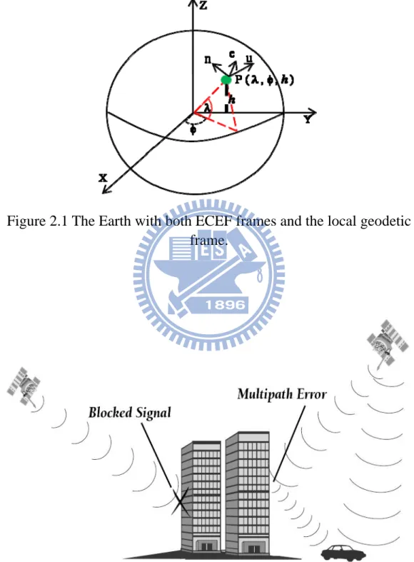
Figure 2-1 The Earth with both ECEF frames and the local geodetic frame 40

Figure 3-1 GPS signal multi-path and blocked by building……….. 40

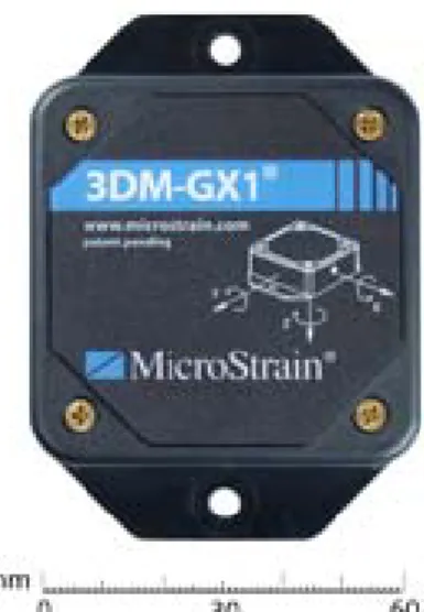
Figure 3-2 MicroStrain@ 3DM-GX1 IMU………... 41

Figure 3-3 GARMIN GPS-18-PC………. 41

Figure 4-1 Operation of the Kalman Filter……… 41

Figure 4-2 Conventional Kalman Filter………. 42

Figure 4-3 Model reference Kalman Filter……… 42

Figure 4-4 Linear/Circular Approximation weighting……..……… 43

Figure 4-5 GPS/IMU data fusion……….………. 43

Figure 5-1 ARTC high speed railway……… 44

Figure 5-2 An oval shape track………. 44

Figure 5-3 Test track coordinate system……… 45

Figure 5-4 Placement of spiral curve………. 45

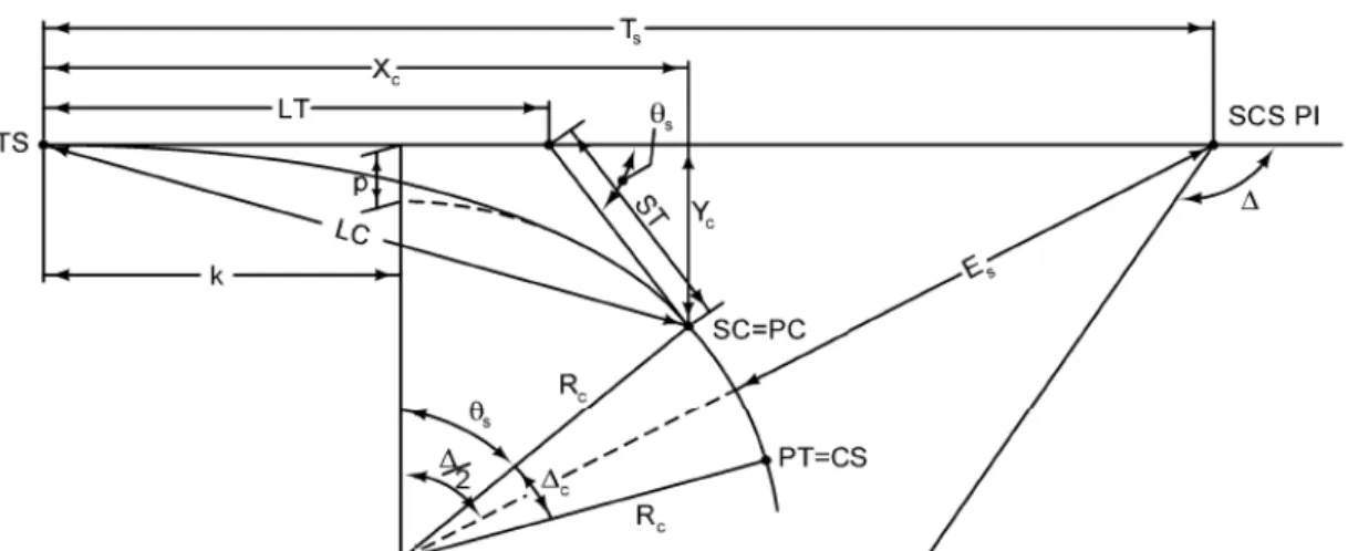
Figure 5-5 Components of a spiral curve………..… 45

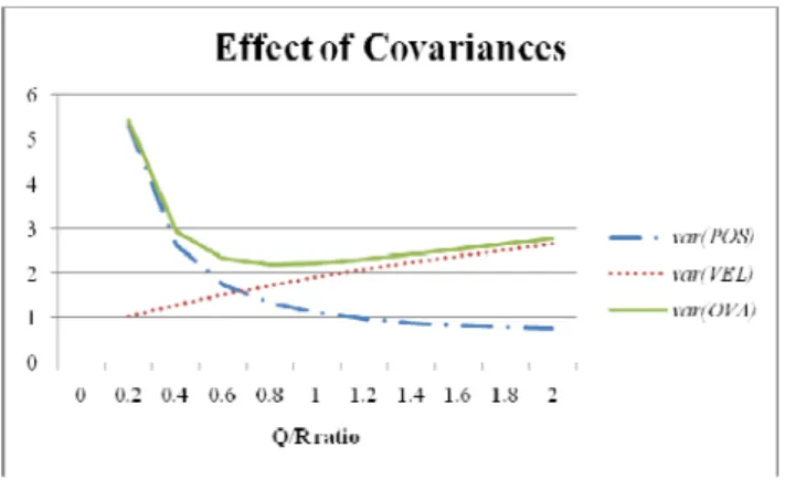
Figure 5-6 Effect of Covariances……….. 46

Figure 5-7 Effect of Fading factor………... 46

Figure 5-8 Effect of GPS/IMU data fusion……… 47

Figure 5-9 The trajectory of vehicle estimated by MRKF in different situations………... 48

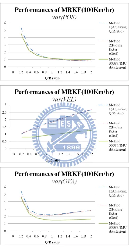
Figure 5-10 MRKF’s performance when the velocity is 100km/hr…………. 49

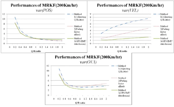
Figure 5-11 MRKF’s performance when the velocity is 200km/hr…………. 50

Figure 5-12 The trajectory of vehicle estimated by MRKF when the velocity is 200km/hr……… 50

Figure 5-13 MRKF’s performance when the velocity is 400km/hr…………. 51

Figure 5-14 The trajectory of vehicle estimated by MRKF when the velocity is 400km/hr……… 51

Chapter 1 Introduction

1.1 Motivation and Objectives

FMCW ( Frequency Modulated Continuous Wave ) radar systems are generally compact and relatively cheap to purchase and to exploit. They consume little power and, due to the fact that they are continuously operating, they can transmit a modest power, which makes them very interesting for military applications. Consequently, FMCW radar technology is of interest for civil and military airborne earth observation applications, especially in combination with high resolution SAR techniques. The novel combination of FMCW technology and Synthetic Aperture Radar (SAR) techniques leads to the development of a small, lightweight, and cost-effective high resolution imaging sensor.

Processing Synthetic Aperture Radar (SAR) images is a non trivial and computationally heavy task. To perform this process in real time is challenging and the final result is highly dependent on the reconstruction of the flight path. This reconstruction is performed with data from the navigation system and an autofocus algorithm. The performance of autofocus algorithms is strongly correlated with the quality of the flight-path reconstruction data produced by the navigation system.

The work here presented describes the Mini-SAR navigation system initial stages of development starting with the motivations to the sensors selection and finalizing with the analysis of the data.

1.2 Background and Literature review

The Global Positioning System(GPS) represents an inexpensive and global method of obtaining the position of a vehicle. Although the measurements are highly subjected to noise, the accuracy can be improved by applying the principle of differential GPS. However, the system gives a low bandwidth, especially when it comes to acceleration and speed, which can be calculated by differentiating the position measurements.

As a contrast, an Inertial Navigation System(INS) only measures the forces acting on an Inertial Measurement Unit(IMU), and can thus be used to calculate both speed and position estimates without differentiating. The INS does not rely on external signals and is therefore not susceptible to jamming not the problem of areas lacking satellite coverage.

There are several reasons why an integration of GPS and an INS is desirable. Generally, and INS gives several advantages that the GPS-system lacks, and vice versa. The INS results are available whenever the GPS measurements are unavailable and the INS measurements are obtained without significant time delay. On the other hand, the GPS corrects the integration error from a stand-alone INS system and allows on-line calibration of IMU errors. So the integration provides real time estimates, as opposed to differentiation.

Chapter 2 Reference Frames and Transformations

2.1 Earth Centered – Earth Fixed

In navigation, several reference frames can be used to present the data. Depending on what navigational system is used to obtain the measurements, different reference systems are usually required.

The Earth Centered, Earth Fixed (ECEF) frame has, as the name suggests, its center in the center of the Earth, and the frame is stationary relative to the surface. Of all the possible combinations of ECEF coordinate systems, two are of particular importance.

This is named the ECEF rectangular system but is usually just referred to as the ECEF system. Its x-axis points through the intersection of the prime median (0o longitude), and equator (0o latitude), its z-axis towards the true north pole, and the y-axis to complete the right hand rule through the intersection of 90 o longitude and equator.

The other representation is called ECEF geodetic frame. This system expresses position in latitude, longitude and height, [φ, λ, h] and is given in the spherical coordinates. The latitude is found by rotating around the z-axis until the x-axis crosses the projection from the position on to the x-y-plane. The longitude is then found by rotating around the y-axis until the x-axis coincides with the vector from the center of the Earth to the position. The height is the distance from the nearest point normal on the assumed altitude.

2.2 Local Geodetic and Body Frame

The local geodetic frame takes basis of making a fictional tangent plane at the origin, just like presenting the globe as a map. The x-axis points north, the y-axis towards east and the z-axis points down, normal onto the ellipsoid, therefore also widely known as the NED-frame (north-east-down). This frame coincides with the geographic frame for a stationary target. The difference between the two is that in the latter frame, the origin is a projection of the platform origin onto the Earth's geodetic. Another version of this frame is the east, north, up-frame (ENU).

The body frame is usually in the center of gravity of the body of the object in question. Its x-axis points towards the defined front of the object, the z-axis points down and the y-axis points right to complete the right hand rule. This frame and the NED-frame are widely used for control purposes.

The frame represents the vehicle states in 6 degrees of freedom (6 DOF) known as surge, sway and heave (u, v, w), and roll, pitch and yaw (φ, λ,

ψ

). Surge, sway and heave are the speed in x, y and z respectively, and roll, pitch and yaw are the vehicle's angular displacement from the NED-frame.

The transformation from ECEF-to-tangent plane coordinates, starts by subtracting the tangent plane origin, given in the ECEF-frame, from the ECEF coordinates, leaving the two planes with the same origin.

(

) (

T

)

T z y x z y x, , ₀, ₀, ₀ x= −

δ

(2.1)

The next step is performing a rotation around the ECEF z-axis until the y-axis is aligned with tangent-plane east, where the λ is the longitude.

( )

( )

( )

( )

⎥ ⎥ ⎥ ⎦ ⎤ ⎢ ⎢ ⎢ ⎣ ⎡ − = 1 0 0 0 0

λ

λ

λ

λ

cos sin sin cos R₁ (2.2)

By performing a new rotation, this time around the aligned y-axis until the new z-axis is aligned with the tangent-plane down where φ is the latitude.

( )

( )

( )

( )

⎥⎥ ⎥ ⎦ ⎤ ⎢ ⎢ ⎢ ⎣ ⎡ − − − = ⎥ ⎥ ⎥ ⎥ ⎥ ⎦ ⎤ ⎢ ⎢ ⎢ ⎢ ⎢ ⎣ ⎡ ⎟ ⎠ ⎞ ⎜ ⎝ ⎛ + ⎟ ⎠ ⎞ ⎜ ⎝ ⎛ + − ⎟ ⎠ ⎞ ⎜ ⎝ ⎛ + ⎟ ⎠ ⎞ ⎜ ⎝ ⎛ + =

φ

φ

φ

φ

π

φ

π

φ

π

φ

π

φ

sin cos cos sin cos sin sin cos R 0 0 1 0 0 2 0 2 0 1 0 2 0 2 2 (2.3)

By combining the two, the complete rotation matrix is obtained.

( ) ( )

( ) ( )

( )

( )

( )

( ) ( )

( ) ( )

( )

⎥⎥ ⎥ ⎦ ⎤ ⎢ ⎢ ⎢ ⎣ ⎡ − − − − − − =

φ

λ

φ

λ

φ

λ

λ

φ

λ

φ

λ

φ

sin sin cos cos cos cos sin cos sin sin cos sin Rt_E 0 (2.4)

2.4 Body-to-Tangent Plane Transformation

By using the Euler angles derived from the body frame and transforming via one axis at a time, and by choosing to start with the rotation around the z-axis the new coordinates

[

x′ y′ z′

]

Tis obtained.

( )

( )

( )

( )

⎥ ⎥ ⎥ ⎦ ⎤ ⎢ ⎢ ⎢ ⎣ ⎡ ⎥ ⎥ ⎥ ⎦ ⎤ ⎢ ⎢ ⎢ ⎣ ⎡ − = ⎥ ⎥ ⎥ ⎦ ⎤ ⎢ ⎢ ⎢ ⎣ ⎡ ′ ′ ′ z y x z y x 1 0 0 0 0

ψ

ψ

ψ

ψ

cos sin sin cos (2.5)

The two remaining axes are applied by the same method, and the body frame coordinates have obtained.

( )

( )

( )

( )

( )

( )

( )

( )

⎥⎥ ⎥ ⎦ ⎤ ⎢ ⎢ ⎢ ⎣ ⎡ ′′ ′′ ′′ ⎥ ⎥ ⎥ ⎦ ⎤ ⎢ ⎢ ⎢ ⎣ ⎡ − = ⎥ ⎥ ⎥ ⎦ ⎤ ⎢ ⎢ ⎢ ⎣ ⎡ ⎥ ⎥ ⎥ ⎦ ⎤ ⎢ ⎢ ⎢ ⎣ ⎡ ′ ′ ′ ⎥ ⎥ ⎥ ⎦ ⎤ ⎢ ⎢ ⎢ ⎣ ⎡ − = ⎥ ⎥ ⎥ ⎦ ⎤ ⎢ ⎢ ⎢ ⎣ ⎡ ′′ ′′ ′′ z y x w v u z y x z y x

θ

θ

θ

θ

θ

θ

θ

θ

cos sin sin cos cos sin sin cos 0 0 0 0 1 0 0 1 0 0 (2.6) (2.7)

And these can be combined by multiplication, yielding

( )

( )

( )

( )

( )

( )

( )

( )

( )

( )

( )

( )

⎥⎥ ⎥ ⎦ ⎤ ⎢ ⎢ ⎢ ⎣ ⎡ − ⎥ ⎥ ⎥ ⎦ ⎤ ⎢ ⎢ ⎢ ⎣ ⎡ − ⎥ ⎥ ⎥ ⎦ ⎤ ⎢ ⎢ ⎢ ⎣ ⎡ − =

θ

θ

θ

θ

θ

θ

θ

θ

ψ

ψ

ψ

ψ

cos sin sin cos cos sin sin cos cos sin sin cos R 0 0 0 0 1 0 0 1 0 0 1 0 0 0 0 b t

( ) ( )

( ) ( )

( )

( ) ( )

( ) ( ) ( )

( ) ( )

( ) ( ) ( )

( ) ( )

( ) ( )

( ) ( ) ( )

( ) ( )

( ) ( ) ( )

( ) ( )

⎥⎥ ⎥ ⎦ ⎤ ⎢ ⎢ ⎢ ⎣ ⎡ + − + + + − − = φ θ φ θ ψ θ ψ φ θ ψ θ ψ φ θ φ θ ψ θ ψ φ θ ψ θ ψ θ θ ψ θ ψ cos cos sin sin sin cos cos cos sin cos sin sin sin cos sin sin sin cos cos sin sin cos cos sin sin cos sin cos cos (2.8)

2.5 GPS Coordinate Systems

The use of a reference ellipsoid allows for the conversion of the ECEF (Earth-Centered, Earth-Fixed) coordinates to the more commonly used geodetic-mapping coordinates (LLA) of Latitude(

ϕ

; in degrees), Longitude (

λ

; in degrees), and Altitude ( h ；in meters). GPS commonly adopts the LLA coordinate system. The conversion between the two reference coordinate systems can be performed using closed formulas. The conversion from LLA to ECEF (in meters) is shown as below.

λ

ϕ

cos cos ) (N h X = + (2.9)

λ

ϕ

sin cos ) (N h Y = + (2.10)

ϕ

sin ) ( N h a b Z = 2₂ + (2.11)

where N is the radius of curvature (meters), defined as

ϕ

2 2 2 2 1 sin a b a a N − − = (2.12)

a and b are the semi-major and semi-minor axes of the reference

ellipsoid of earth, respectively. h denotes the height of the position above the reference ellipsoid. According to the WGS84 parameters, we have

6378137 =

2.5 Local Projection

According to the LLA coordinate system, a small region may be identified with a center for projection (

ϕ

c,

λ

c) onto a flat mapping

surface called the x-y plane as follows. ) c x=

κ

_λ(

λ

−

λ

(2.13) ) c y =

κ

_φ(

ϕ

−

ϕ

(2.14)

The y-axis local project is pointing to the north pole of the earth when the center of projection is on the north semi-hemisphere. The x-axis is determined through the right-hand law with the thumb pointed to the north pole.

κ

_λand

κ

_ϕare the mapping constants from LLA coordinate to local projection, which are defined

λ

κ

=

π

(N +h)cos

ϕ

/180 (meter/degree) (2.15) ϕ

κ

= ( 1₂ (a2h b2N)2cos2

ϕ

(a4N2 2a4Nh)sin2

ϕ

)/180 a π + + − (meter/degree) (2.16)

Chapter 3 GPS/IMU

3.1 GPS

The GPS is part of a satellite-based navigation system developed by

the U.S. Department of Defense under its NAVSTAR satellite program[4]. The fully operational GPS includes 28 or more active satellites approximately uniformly dispersed around six circular orbits with four or more satellites each. The orbits are inclined at an angle of 55o relative to the equator and are separated from each other by multiples of 60o right ascension. The orbits are nongeostationary and approximately circular, with radii of 26,560 km and orbital periods of one-half sidereal day (about 11.967hrs). Theoretically, three or more GPS satellites will always be visible from most points on the earth’s surface, and four or more GPS satellites can be used to determine an observer’s position anywhere on the earth’s surface 24hrs per day.

3.1.1 GPS Signals

Each GPS satellite transmits two spread spectrum, L-band carrier signals – an L1 signal with carrier frequency f1 = 1575.42 MHz and an L2

signal with carrier frequency f2 = 1227.6 MHz. These two frequencies are

integral multiples f1 = 1540 f0 and f2 = 1200 f0 of the base frequency f0 =

keying(BPSK), modulated by two pseudorandom noise(PRN) codes in phase quadrature, designated as the C/A-code and P-code. The L2 signal

from each satellite is BPSK modulated by only the P-code. Both frequencies are available for all users, but due to encryption of the P-code, only the C/A-code is usable by the public.

3.1.2 Sources of Errors

Civilian GPS receivers have potential position errors due to the result of the accumulated errors[5] due primarily to some of the following sources:

1. Ionosphere and troposphere delays:

The satellite signal slow as it passes through the atmosphere. The system uses a built-in model that calculate an average, but not an exact, amount of delay.

2. Signal multi-path:

When the GPS signal is reflected off object such as tall buildings or large rock surfaces before it reaches the receiver.

3. Receiver clock errors:

Since it’s not practical to have an atomic clock in your GPS receiver, the built-in clock can have very slight timing errors.

The more satellites the receiver can “see”, the better the accuracy. Anything can block signal reception, causing position errors or possibly no position reading at all, like figure 3.1.

6. Satellite geometry/shading:

Ideal satellite geometry exists when the satellites are located at wide angles relative to each other. Poor geometry results when the satellites are located in a line or in a tight grouping.

7. Intentional degradation of satellite signal:

The U.S. military’s intentional degradation of the signal is known as “Selective Availability”(SA) and is intended to prevent military adversaries from using the highly accurate GPS signals. SA accounts for the majority of the error in the range. SA was turned off May 2, 2000, and is currently not active. This means we can expect typical GPS accuracies in the range of 6-12 meters.

3.1.3 Velocity Measurements

The integration is performed in two different frames, depending on the measurement. For position, ECEF geodetic [φ, λ, h] is used, while for speed, the tangent-plane (NED) has been chosen. In order to transform the GPS data, the position, already given in ECEF geodetic coordinates, is differentiated. To transform the speed, yielding that:

(

) ( )

⎥ ⎥ ⎥ ⎦ ⎤ ⎢ ⎢ ⎢ ⎣ ⎡ ⎥ ⎥ ⎥ ⎦ ⎤ ⎢ ⎢ ⎢ ⎣ ⎡ − + + = ⎥ ⎥ ⎥ ⎦ ⎤ ⎢ ⎢ ⎢ ⎣ ⎡ h h R h R v v v D E N & & &

λ

φ

φ

λ φ 1 0 0 0 0 0 0 cos (3.1)

3.2 Inertial Measurement Unit(IMU)

The IMU chosen is the MicroStrain@ 3DM-GX1(Figure 3.2). It consists of three accelerometers, three gyros and three magnetometers, and giving acceleration in 6 degrees of freedom(6 DOF) and position in 3 DOF. This IMU performs an accelerometer bias stability of 0.01G, where the G is the Earth’s gravitational constant, and 0.7o/sec for the gyros. And the sensors have bandwidth of 100hz, and transmit data over an RS-232 serial line.

3.3 GPS Module

The GPS module chosen is GARMIN GPS-18-PC(Figure 3.3). This module operates at 8 – 30V, and transmits data through RS-232. It has position accuracy at 15m, or 3m with Wide Area Augmentation System(WAAS) enabled. And its update rate is 1Hz, so it can transmit 1 record per second.

Chapter 4 Kalman Filter

The Kalman Filter is an optimal, linear state estimator, able to estimate the full system state, depending on incomplete and noisy measurement series. The theory of the filter dates back to 1960, when Rudolf Kalman proposed the Filter to NASA for the Apollo Program. The Kalman filter is essentially a set of mathematical equations that implement a predictor-corrector type estimator that is optimal in the sense that it minimizes the estimated error covariance—when some presumed conditions are met. Since the time of its introduction, the Kalman Filter has been the subject of extensive research and application, particularly in the area of autonomous or assisted navigation. The filter comes in many different forms, but the one most relevant for this work is the discrete Kalman Filter, which also will be the one most thoroughly investigated.

4.1 Conventional Kalman Filter Implementation

The Kalman filter addresses the general problem of trying to estimate the state x∈Rn of a discrete-time controlled process that is governed by the linear stochastic difference equation. The basic operation of Kalman Filter is shown in Figure 4.1 and 4.2.

The a priori estimation:

1 1 − − − _{= +} k k k Axˆ w xˆ (4.1) The a posteriori estimation:

) v xˆ H z ( K xˆ xˆ_k = _k− + _k − _k− + _k (4.2) The random variables w and_k v represent the process and _k measurement noise, respectively. They are assumed to be independent of each other, white, and with normal probability distributions

) Q , ( ~ ) w ( N 0 p ) R , ( ~ ) v ( N 0 p

In practice, the process noise covariance Q and measurement noise covariance P matrices might change with each time step or measurement. The Kalman gain K is obtained from the updating scheme:

1 − − − ₊ = H (H H R) K_k P_k T P_k T (4.3) Where Q A ) KH I ( A − + = − − − T k k P P ₁ (4.4) Problem of the conventional Kalman Filter based position estimation is that the update frequency is determined by when the sensor input z _k frequency. If the sampling frequency of z is low, for example sampling _k frequency is 1Hz for the GPS sensor, the position error can be as large as 100 m for a vehicle running at speed of 100km/hr.

combine the GPS and IMU with different data rate. The basic operation of Model reference Kalman Filter is shown in Figure 4.3.

Discrete form:

k k

k (I B)Ax Bz

x = − ₋₁ + (4.5) Where B is diagonal matrix and the diagonal entries can only be Boolean (0 or 1).

The a priori estimation:

1 1 − − − _{= +} k k k Axˆ w xˆ The a posteriori estimation:

) v xˆ H (z K xˆ xˆ_k = _k− + _k− _k− + _k When z comes from GPS/IMU sensor, i.e. k

⎥ ⎥ ⎥ ⎥ ⎦ ⎤ ⎢ ⎢ ⎢ ⎢ ⎣ ⎡ = y x y x k & & z

The sampling rate of IMU is higher than that of the GPS in practice. Assuming that the sampling time of IMU is T, the system matrix of the plant may be written as follows.

⎥ ⎥ ⎥ ⎥ ⎦ ⎤ ⎢ ⎢ ⎢ ⎢ ⎣ ⎡ = 1 0 0 0 0 1 0 0 0 1 0 0 0 1 T T A

⎥ ⎥ ⎥ ⎥ ⎦ ⎤ ⎢ ⎢ ⎢ ⎢ ⎣ ⎡ = k k k k k y x y x & & x

The sensor matrix compares only the position differences as follows.

⎥ ⎦ ⎤ ⎢ ⎣ ⎡ = 0 0 1 0 0 0 0 1 H 2 2 2 2 2 0 0 x R R R _I R

σ

σ

σ

₌ ⎥ ⎦ ⎤ ⎢ ⎣ ⎡ = ; ⎥ ⎦ ⎤ ⎢ ⎣ ⎡ = ⎥ ⎥ ⎥ ⎥ ⎦ ⎤ ⎢ ⎢ ⎢ ⎢ ⎣ ⎡ = 2 2 2 2 2 2 2 0 0 0 0 0 0 0 0 0 0 0 0 0 0 x Q x Q Q I 0 Q

σ

σ

σ

;

Matrix B may be written into the following form.

⎥ ⎦ ⎤ ⎢ ⎣ ⎡ = I I B

δ

χ

0 0 where ⎩ ⎨ ⎧ = else GPS by updated is position if 0 1

χ

⎩ ⎨ ⎧ = else GPS/IMU by updated is velocity if 0 1

δ

The Kalman gain K is obtained from the updating scheme:

1 − − − ₊ = H (H H R) K_k P_k T P_k T

4.2.1 Effect of Covariances

The update scheme of Kalman gain is

1 − − − ₊ = H (H H R) K_k P_k T P_k T where Q A ) H K I ( A − + = − − − − T k k k P P _{1 1}

Assuming that the priori error covariance P_k−and Kalman gain take the following forms in the steady state.

⎥ ⎦ ⎤ ⎢ ⎣ ⎡ = × × × × − 2 2 22 2 2 12 2 2 12 2 2 11 I I I I p p p p P_k ⎥ ⎦ ⎤ ⎢ ⎣ ⎡ = × × 2 2 2 2 2 1 I I k k K_k We obtain that 0 4 4 8 4 4

η

2k₂4 −

η

Tk₂3−

η

k₂2 − Tk₂ + = (4.6) Where ₂ 2 Q R

σ

σ

η

= . k₂(velocity Kalman gain) is obtained from the fourth

order polynomial equation (4.6). k₁ (position Kalman gain) may be obtained from the following relation (Appendix C).

η

2 2

1 1 k

k = − (4.7) The Kalman gains are function of the ratio of the position covariance and velocity covariance,

η

, not the independent values. That is for the systems with the same ratio

η

, the Kalman gains are identical, which

may be considered as the water bed effect.

4.2.2 Adaptive Filtering with Fading Factor

The Kalman gain K is obtained from the updating scheme:

1 − − − ₊ = H (H H R) K_k P_k T P_k T Where Q ) B I ( A A ) B I ( − − + = − T T k k P P (4.8.1) or Q ) B I ( A ) H K I ( A ) B I ( − − − + = − − − − T T k k k P P _{1 1} (4.8.2)

Since the diagonal entry of matrix B is a function of sensor data status, the updating scheme of P_k− may then be simplified into

' Q A ) H K I ( A − + = − − − − T k k k P P _{1 1} (4.9) Where Q ) ( ' Q max d d

α

− = 1 (4.10) max

d denotes the maximum lost of GPS data endurable to the system. d

denotes the current loss of GPS data count. The equivalent covariance

'

Q of the process noise is monotonically decreasing with d. 10<

α

≤ denotes the weight corresponds to the loss GPS data rate, the equivalent

count is based on a given sampling time T . The situation when the loss data count d >d_max implies that the GPS is down or the vehicle is coming into a full stop thus the position cannot be further updated by the GPS. In such case, one must terminate the position estimation process and set x_k =HTz_k.

4.2.3. GPS/IMU Data Fusion

The GPS data is not only useful for updating the position but also the velocity component in zk . A simple forward difference method,

known as the linear approximation, may be used for the velocity approximation purpose as shown in Figure 4.4. Also the circular approximation based three known local coordinates may also be used to perform the précised estimation especially when the vehicle is moving on the circular track.

The other information may be obtained from the linear and circular approximation are the information of the yaw angle of the vehicle which may be simply written as follows.

) tan( x y GPS & & =

θ

Since the GPS data refreshing rate is lower than the IMU refreshing rate, 1 to 7 in our study, the IMU accelerometer may be used to update the velocity estimated by GPS. The IMU gyro yields the yaw angle

θ

_gyro of the vehicle can be used to determine the direction of the velocity. When

the new velocity is obtained, we will set

δ

in matrix B to be 1.

When the vehicle is running on the circular path, the insufficient sampling rate of GPS will cause the position component of zk be zero

for a long time, the position estimation of xˆ_k relies entirely on the

velocity component of zk. However, the direction of the velocity must

according to the IMU updates. Figure 4.5 shows that the process of GPS and IMU data fusion. In case of high speed turning, the IMU is not fast enough to perform the immediately update, the vehicle will then tend to outrun the circular path. Since The IMU gyro also yields the yaw angular rate

θ

&gyro of the vehicle, a yaw compensation scheme proposed

according to the yaw angular rate as follows may be useful to prevent the outrun situation.

Chapter 5 Experiment and Comparisons

5.1 Test Track Coordinate System

The benchmark is based on the raw DGPS data acquired from ATRC high speed test track, as shown in Figure 5.1, consists of three oval shape runways. The total length of the runway is around 3575 m including 2000 m straight way and 1575m circular way (radius of the middle runway is about 250m). The DGPS data is received on a car which runs in a nearly constant speed, say 100 km/hr, on the runway. The sampling time of DGPS is 1 second and the sampling time of the IMU is 140 ms. The geodetic reference (datum) used for GPS is the World Geodetic System 1984 (WGS84) including the latitude and longitude of the geographic coordinates. Equivalently, the rate of IMU data is 3.89m per data received and the rate of DGPS data is 28m per data received when the car speed is 100km/hr which is nearly the resolution of DPGS used in this work. Knowing the symmetry the oval shape test track, we are able to estimate the center coordinate of the test road by summing all the DGPS data and then dividing the total coordinate value by the number of data taken, i.e.

∑

= = = n j j c n ₁ 1

_λ

λ

λ

=24.06764624

∑

= = = n j j c n ₁ 1

_ϕ

ϕ

ϕ

=120.382617

based on eq.(2.9) and (2.10) as follows. c X = -2947234.9 c Y = 5026933.9 c Z = 2585262.1

Substituting the center point into the local project coefficient indicated in eq. (2.13) and (2.14), we have

λ

κ = 101698.51

ϕ

κ = 110760.24

According to eq. (2.13) and (2.14), we obtain that

j

x = 101698.51(

λ

j −

λ

c)

j

y =110760.24(

ϕ

j −

ϕ

c)

An oval shape track with known dimension consists of 4 segments which are 2 line segments, as shown in Figure 5.2,

Segment #1: x−x_o,1 + ytan

θ

=0 (5.1) Segment #2: (x−x_o,2)2 +(y− y_o,2)2 −R2 =0 (5.2) Segment #3: x−x_o,3 + ytan

θ

=0 (5.3) Segment #4: (x−x_o,4)2 +(y− y_o,4)2 −R2 =0 (5.4) where x_o and x_o are the linear offsets of the line segment #1 and #3

Since the line segments are constrained by the shape of the track, we have

θ

cos , , R x x_o3 = _o1 − 2 (5.5) The centers of the circular segments are also constrained by the shape of the track as follows.

θ

θ

) tan cos ( _{, ,} ,2 1 2 0 o yo R x x = − − (5.6) and

θ

θ

) tan cos ( _{, ,} ,4 1 4 0 o yo R x x = − − (5.7) Substituting eq. (5.5), (5.6) and (5.7) into eq.(2.9) to (2.12), there are totally five independent unknown parameters in eq. (2.9) to, (2.12), which may be integrated into a vector form as follows.

[

]

T o o o R y y x _{,1 ,2 ,4} U =

θ

One may write the four segment equations as follows. 0 1 1,j(U;xj,yj)= xj −xo, + yj tan

θ

= f (5.8) 0 2 2 2 2 2 1 2 = − − + y + y − y −R = R x x y x f _{j j j j o} ) _o tan ) ( _{j o} ) cos ( ( ) , ; U ( _{, , ,} ,

θ

θ

(5.9) 0 2 1 3 = − −

θ

)+ tan

θ

= cos ( ) , ; U ( _, ,j j j j o yj R x x y x f (5.10) 0 2 2 4 2 4 1 4 = − − + y + y − y −R = R x x y x f _{j j j j o} ) _o tan ) ( _{j o} ) cos ( ( ) , ; U ( _{, , ,} ,

θ

θ

(5.11)

In order to linearize the above equations, we let U U~ U = +Δ (5.12) where

[

]

T o o o R y y x _,1 ~ ~ ~ _,2 ~ _,4 ~ U~ =

θ

[

]

T o o o R y y x _{,1 ,2 ,4} U = Δ Δ Δ Δ Δ Δ

θ

0 = Δ ∇ + ≈ ≡ (U; , ) (U~) (U~) U ) U ( _{, , ,} , T j i j i j j j i j i f x y f f f

The above equation yields that

) U~ ( U ) U~ ( _, , i j T j i f f Δ = ∇ − (5.13) It is obtained that

[

1 2 0 0 0

]

1

θ

~ sec ) U~ ( , j T j y f = − ∇ − ⎥ ⎥ ⎥ ⎥ ⎥ ⎥ ⎦ ⎤ ⎢ ⎢ ⎢ ⎢ ⎢ ⎢ ⎣ ⎡ − + − − − − − − − = ∇ − 0 2 1 2 2 2 2 2 2 2 2 2 2 2 )) ~ ( ~ tan ) ~ (( ) ~ sec ) ~ ( ( ) ~ tan ~ sec ~ ~ sec )( ~ ( ) ~ ( ) U~ ( , , , , , , , o j o j o j o o j o j j y y x x x x R y x x x x f

θ

θ

θ

θ

θ

⎥⎦ ⎤ ⎢⎣ ⎡ − − − = ∇ − ₃ 1 2 2 2 0 0

θ

θ

θ

θ

_~ cos ~ tan ~ sec ~ ~ sec ) U~ ( , y R f T _j j ⎥ ⎥ ⎥ ⎥ ⎥ ⎥ ⎦ ⎤ ⎢ ⎢ ⎢ ⎢ ⎢ ⎢ ⎣ ⎡ − + − − − − − − − = ∇ − )) ~ ( ~ tan ) ~ (( ) ~ sec ) ~ ( ( ) ~ tan ~ sec ~ ~ sec )( ~ ( ) ~ ( ) U~ ( , , , , , , , 4 4 4 2 4 4 4 4 2 0 1 2 2 2 o j o j o j o o j o j j y y x x x x R y x x x x f

θ

θ

θ

θ

θ

where

θ

θ

~ tan ~ ) ~ cos ~ ~ ( ~ , , ,2 o1 o2 o y R x x = − − and

θ

θ

~ tan ~ ) ~ cos ~ ~ ( ~ , , ,4 o1 o4 o y R x x = − −

D U

CΔ = (5.14) MatrixCand vectorD may be assembled as follows.

⎥ ⎥ ⎥ ⎥ ⎦ ⎤ ⎢ ⎢ ⎢ ⎢ ⎣ ⎡ = 4 3 2 1 D D D D D ⎥ ⎥ ⎥ ⎦ ⎤ ⎢ ⎢ ⎢ ⎣ ⎡ = ) U~ ( ) U~ ( D , , , , e i s i q i q i i f f M ⎥ ⎥ ⎥ ⎥ ⎦ ⎤ ⎢ ⎢ ⎢ ⎢ ⎣ ⎡ = 4 3 2 1 C C C C C

[

T

]

q i T q i i f _is f _ie U) ~ ( ) U~ ( C , , , , −∇ ∇ − = _L

The least square solution yields that

D C ) C C ( U = T −1 T Δ (5.15) The iteration among procedures according to eq. (5.15) , eq. (5.12), and

U

U~ = ends when ΔU ≤

ε

and the Hessian condition is satisfied for the minimum, we obtainU≈ . According to the least square result of U~ U~ , the test track coordinate system, as shown in Figure 5.3, including

c

x , y , L , R , and _c

θ

may be obtained that

(

) (

)

2 4 2 2 4 2 , , , , ~ ~ ~ ~ o o o o x y y x L = − + − R R = ~

θ

θ

= ~

2 4 2 , , ~ ~ o o c x x x = + 2 4 2 , , ~ ~ o o c y y y = +

The nominal test track may be written into a formula as follows in terms of the parameter u . ) , , , , , ( g x y L R u y x c c

θ

= ⎥ ⎦ ⎤ ⎢ ⎣ ⎡

5.2 Spiral Curves and DGPS Inaccuarcy

The difference f_{i, j}(U~) between the DGPS data and the least square test track may be calculated. The residue of vector D may form a trajectory variance that

D DT

=

μ

The trajectory variance

μ

contains not only the DGPS inaccuracy but also the spiral curves. Spiral curves are generally used to provide a gradual change in curvature from a straight section of road to a curved section. They assist the driver by providing a natural path to follow. Spiral curves also improve the appearance of circular curves by reducing the break in alignment perceived by drivers[2]. Figure 5.4 shows the

map the local position (x , _j y ) onto the test track parameter _j u that _j minimize the offset from the test track, i.e.

) , , , , , ( g min ) , , , , , ( g x y L R u y x u R L y x y x c c j j u u u c c j j j

θ

θ

_⎥− ⎦ ⎤ ⎢ ⎣ ⎡ = − ⎥ ⎦ ⎤ ⎢ ⎣ ⎡ =

The trajectory error for local position may be written as ) , , , , , ( g x y L R u y x e _{c c} j j j ⎥−

θ

⎦ ⎤ ⎢ ⎣ ⎡ =

It may be possible to use the cumulative moving average to calculate the spiral curves as follows.

1 j 2 2 + =

∑

+ = − = / / j p k j p k k j e e , p is an even integer.

The maximum DGPS inaccuracy is then evaluated as follows. ) ( max ,n j j j GPS e e e = − =1

Since the particular type of the DGPS we used in this study is with 3 meter inaccuracy, we will choose p such that e_GPS = 3m.

5.3 Experiments and Analysis

In order to increase the accuracy, there are 3 methods we can adjust. Following the process below and input these values, there will be a best final result.

1. Adjusting the Q/R ratio.

3. GPS/IMU data fusion and Yaw compensation.

There are 3 output values that we can evaluate the results. The Position-variance is the error of position after our process. The Velocity-variance is the error of velocity after our process. The Overall-variance is equal to var

(

POS

)

2 +var

(

VEL

)

2 . And the values of these variances are the smaller the better.

5.3.1 Adjusting the Q/R ratio

In Kalman Filter, the purpose of the weights is that values with better estimated uncertainty are “trusted” more. The Q denotes process noise covariance(Velocity-covariance), and the R denotes measurement noise covariance(Position-covariance). In this Model reference Kalman Filter(MRKF), the smaller covariance means that we “trust” it more. The Q/R ratio is equal to ) ( covariance Position ) ( covariance Velocity R Q − −

. Figure 5.6 shows that

the Q/R ratio getting bigger will causes the var(POS) getting smaller but it also causes the var(VEL) getting bigger. In our process, the velocity of vehicle is about 3m per data and the accuracy of DGPS is about 3m, so the ratio between R and Q will be the best result at about 1:1.

shading of buildings. In order to keep MRKF working on the situation of GPS loss data count, we should input the adaptive Fading factor. Increasing Fading factor means the covariance Q of process noise is monotonically decreasing. In other words, because of the GPS loss data count, we trust the measurement process less and estimation process will be trusted more. Figure 5.7 shows that the bigger Fading factor will increase the Position accuracy but decrease the Velocity accuracy, and the best Fading factor is about 0.5.

5.3.3 GPS/IMU data fusion and Yaw compensation

The GPS data is not only updating the position but also the velocity component in z .When we use GPS data to update the velocity _k component in z , the velocity accuracy will be dramatically increased. In _k our application, the vehicle is not only moving on the straight line but also on the circular track. In order to know the direction of velocity, we have to use the IMU. The accelerometer of IMU may be used to update the velocity estimated by GPS and the gyro of IMU yields the yaw angle

gyro

θ

of the vehicle can be used to determine the direction of the velocity. As the time goes on, the gyro will yield some drifts and cause the error of yaw angular rate. In order to correct the effect of drift, we should add the yaw compensation. Figure 5.8 shows the GPS/IMU data fusion and the yaw compensation will increase the velocity accuracy but not causing the error of position, and the overall variance will be decreased to 1.5.

5.3.4 GPS loss data count or the vehicle is moving faster

The GPS data updating rate is 1Hz and the velocity of the vehicle is 100km/hr in this work. But the GPS sensor may loss data by some reasons, like bad weather or shading of buildings. If GPS loss data count happened and the updating rate down to 1/2 Hz, then our GPS position information received will be 200km per point. In other words, the vehicle moving faster is just like the lower GPS updating rate. Figure 5.9 shows the trajectories of vehicle reproduced by MRKF in different situations. We can find that the estimation error occur when the vehicle is moving in circular track. In order to increase the accuracy of MRKF when vehicle is moving faster, reducing the estimation error in circular track is very important.

5.3.5 Increasing MRKF accuracy in different situations

Since we know that reducing the estimation error in circular track is very important, there are 3 methods we can adjust to increase the MRKF accuracy. Figure 5.11 and 5.12 represents the velocity of vehicle is 200km/hr (or GPS data updating rate is 1/2Hz). Figure 5.13 and 5.14

estimated velocity is seriously distortion and the estimated trajectory is overshoot. In method 2, the purpose of Fading factor is making MRKF keeps working on the situation of GPS loss data count. The trajectory in circular track is more close to the real track and the velocity variance may dramatically be reduced. In method 3, we use IMU accelerometer to update the estimated velocity and IMU gyro to obtain the information of direction. The GPS/IMU data fusion can both reduce the error of estimated position and velocity, the estimated trajectory may be more closed to the real track, especially in the circular track. Figure 5.15 shows the performances of MRKF in different situations. The error of estimated velocity can be reduced in every step, but the estimated position accuracy can’t be obviously increased. After our adjusting process, we can obtain the best result of MRKF and the accuracy can be increased in any situation.

Chapter 6 Conclusion

In this work, we discussed an enhanced fusion algorithm, MRKF (Model Reference Kalman Filter), which is a loosely coupled GPS/IMU system integrated by a Kalman Filter to estimate the position, heading, and velocity of a car. A dynamic reference model was used as the process model in order to enhance the performance at high speeds and during turns, and it can combine the GPS and IMU with different data rate. The reduced-order Kalman Filter is a simple system and it’s feasible for real-time application on MCU or DSP. We analyzed the performance of the filter using about 100 Km/hr of experimental tests carried out in environments with good and bad GPS coverage. So, if any conclusion is to be made, the IMU is clearly not performing at such a level that any successful integration can be made, at least not for USV. The solution could work to some extent in a car or similar, where the external affect on the track is reduced(Spiral curves and driver behavior). The gyro of IMU is pretty useful, and can be used directly as a compass.

Through experiments and comparison of their performance, a conclusion can be drawn that the MRKF is much more robust than the conventional Kalman Filter in several situations including high speed and during turns, short GPS outrage and low-cost IMU. The error of position can be reduced to less than 1.2 m, the error of velocity can be reduced to

Finding the best Fading factor can dramatically reduce the error of velocity and doesn’t affect the position accuracy, and the estimated trajectory can be more close to the real track. GPS/IMU data fusion and Yaw compensation can increase the accuracy both in position and velocity, especially in the circular track. Through these three methods, we can increase the accuracy not only in position but also in velocity at different situations.

Therefore, it is expected that the MRKF is superior to the conventional Kalman Filter in the state estimation of GPS/IMU integration navigation. It based a good foundation for accurate and robust processing of SAR systems. Its low-cost is also fit to the requirement of Mini-SAR navigation system.

Appendix A.

2 2 2 ) (sin ) cos ) (( ) (

ϕ

λ

ϕ

ϕ

ϕ

d X N h d X X _⎟⎟ = + ⎠ ⎞ ⎜⎜ ⎝ ⎛ ₋ ∂ ∂ + 2 2 2 ) (sin ) sin ) (( ) (

ϕ

λ

ϕ

ϕ

ϕ

d Y N h d Y Y _⎟⎟ = + ⎠ ⎞ ⎜⎜ ⎝ ⎛ ₋ ∂ ∂ + 2 2 2 2 2 ) (cos ) ( ) (

ϕ

ϕ

ϕ

ϕ

a N h d b Z d Z Z _⎟⎟ = + ⎠ ⎞ ⎜⎜ ⎝ ⎛ ₋ ∂ ∂ +

ϕ

ϕ

ϕ

ϕ

ϕ

ϕ

ϕ

ϕ

ϕ

ϕ

ϕ

ϕ

ϕ

ϕ

ϕ

ϕ

ϕ

ϕ

ϕ

ϕ

2 2 2 2 4 2 4 2 4 2 4 2 4 2 2 2 2 4 2 4 2 4 4 2 4 2 2 2 2 2 2 2 4 4 2 4 2 2 2 2 2 2 4 4 4 2 2 2 2 2 2 2 2 4 4 4 2 2 2 2 2 2 2 4 4 4 2 2 2 2 2 2 2 2 2 4 4 2 2 2 2 2 2 2 2 4 4 2 2 2 2 2 2 2 2 4 4 2 2 2 2 2 2 2 2 1 2 2 2 1 2 1 2 2 2 2 2 2 2 2 2 2 2 2 2 cos ) ( sin ) ( cos ) ( cos ) ( ) ( cos ) ( cos ) ( ) ( cos ) ( ) ( ) ( cos ) ( cos ) ( sin ) ( cos ) ( sin ) ( cos ) ( sin ) ( cos ) ( sin ) ( Nh b a N b h a Nh a N a Nh a Nh b a N a N b h a Nh a N a a Nh a b a N a b h N a a Nh a a b N a a b h N h Nh N Nh a a b Nh N a a b N h Nh a a b Nh N a a b N h Nh N h Nh a b N a b h Nh N h Nh a b N a b h Nh N h Nh a b N a b h Nh N Z Y X d + + + − = − + − + + + = − + − + + = − + − + + = + + + − + + − + = + − + + − + + + + = + + + + + = + + + + + = + + + + + = ⎟⎟ ⎠ ⎞ ⎜⎜ ⎝ ⎛ ∂ ∂ + ⎟⎟ ⎠ ⎞ ⎜⎜ ⎝ ⎛ ∂ ∂ + ⎟⎟ ⎠ ⎞ ⎜⎜ ⎝ ⎛ ∂ ∂

Appendix B.

Latitude (

ϕ

) Clake 1866 Ellipsoid International (Hayford) Ellipsoid Snyder 1987 This paper 2010 90 111,699.4 111,700.0 111,694.0 111,694.0 85 111,690.7 111,691.4 111,685.4 111,685.5 80 111,665.0 111,665.8 111,659.9 111,660.2 75 111,622.9 111,624.0 111,618.4 111,618.9 70 111,565.9 111,567.4 111,562.0 111,562.8 65 111,495.7 111,497.7 111,492.6 111,493.7 60 111,414.5 111,417.1 111,412.3 111,413.7 55 111,324.8 111,327.9 111,323.5 111,325.2 50 111,229.3 111,233.1 111,229.1 111,230.9 45 111,130.9 111,135.4 111,131.8 111,133.7 40 111,032.7 111,037.8 111,034.6 111,036.5 35 110,937.6 110,943.3 110,940.6 110,942.2 30 110,848.5 110,854.8 110,852.4 110,853.9 25 110,768.0 110,774.9 110,772.9 110,774.0 20 110,698.7 110,706.0 110,704.3 110,705.0 15 110,642.5 110,650.2 110,648.7 110,649.2 10 110,601.1 110,609.1 110,607.8 110,608.0 5 110,575.7 110,583.9 110,582.7 110,582.8 0 110,567.2 110,575.5 110,574.3 110,574.3

Appendix C.

1 − − − ₊ = H (H H R) K_k P_k T P_k T ⎥ ⎦ ⎤ ⎢ ⎣ ⎡ + = × × 2 2 12 2 2 11 2 11 1 I I K p p p _R k

σ

2 11 11 1 R p p k

σ

+ = 2 11 12 2 R p p k

σ

+ = Where Q A ) KH I ( A − + = − − − T k k P P ₁ ⎥ ⎦ ⎤ ⎢ ⎣ ⎡ = × × × × 2 2 2 2 2 2 2 2 I 0 I I A T ⎥ ⎦ ⎤ ⎢ ⎣ ⎡ = × × × × − 2 2 22 2 2 12 2 2 12 2 2 11 I I I I p p p p P_k ⎥ ⎦ ⎤ ⎢ ⎣ ⎡ = × × 2 2 2 2 2 1 I I k k K_k

[

_2×2 0

]

= I H 2 2 2 x R I R=

σ

2 2 2 x Q T I HQH =

σ

⎥ ⎦ ⎤ ⎢ ⎣ ⎡ + + − + + + − + − − + + + − − = + ⎥ ⎦ ⎤ ⎢ ⎣ ⎡ + + ⎥ ⎦ ⎤ ⎢ ⎣ ⎡ − − − = + ⎥ ⎦ ⎤ ⎢ ⎣ ⎡ ⎥ ⎦ ⎤ ⎢ ⎣ ⎡ ⎥ ⎦ ⎤ ⎢ ⎣ ⎡ − − ⎥ ⎦ ⎤ ⎢ ⎣ ⎡ = + − = × × × × × × × × × × × × × × × × × × × × × × × × × × × × − − − 2 2 2 22 12 2 2 2 22 12 12 11 2 2 2 22 12 2 1 2 2 22 12 12 11 2 1 2 2 22 2 2 22 12 2 2 12 2 2 12 11 2 2 2 2 2 2 2 2 2 2 1 2 2 2 2 2 2 2 2 2 2 22 2 2 12 2 2 12 2 2 11 2 2 2 2 2 2 2 2 2 1 2 2 2 2 2 2 2 2 1 1 1 1 1 I ) ( I )) ( ) ( ( I ) ) (( I )) ( ) )( (( Q I I ) ( I I ) ( I I I I ) ( Q I I 0 I I I I I I I 0 I ) ( I 0 I I Q A ) KH I ( A Q T k k p p k Tp p Tp p k Tp p T k k Tp p T Tp p T k k p Tp p p Tp p k T T k k T p p p p k k T P P

σ

2 2 12 k p =

σ

Q ) ( ) ( T k k T k T k k p Q _Q 2 1 2 2 2 1 2 22 = 1+ + =

σ

σ

) ( ₂ 2 1 2 11 k k p =

σ

_Q 11 22 12 12 11 2 1 1−k −k T)(p +Tp )+T(p +Tp ))= p (( 0 1 _{1 2 12 12 22} 11 2 1 − + − − + + = − ) ( ) ( ) ( k k T p k k T Tp T p Tp 0 2 2 1 2 1 − + = − T k k T k k )( ) ( 0 2 ₂ 1 2 2 1 +k k T − Tk = k 2 8 ₂ 2 2 2 2 1 Tk T k T k k =− + +

(

)

2 2 2 2 2 2 2 2 8 2 2− k

η

+k T =k T + Tk 2 2 2 2 1 2 11 12 2 1 Q R R _k k k p p k

σ

σ

σ

+ = + =

References

[1] Lorga J. F. M., Rossum W. van, van Halsema E., Chu Q. P and Mulder J. A., “The Development of a SAR Dedicated Navigation

System: From Scratch to the First Test Flight.”, IEEE Position and

Location Symposium, Monterey Ca, USA, 2004.

[2] Spiral curves, Design Manual Chapter 2 Alignments, Iowa Department of Transportation Office of Design, 2010.

[3] J. A. Farrell and M. Barth., “The Global Positioning System & Inertial

Navigation.”, R. R. Donneley & Sons Company, 1999.

[4] M. S. Grewal, L. R. Weill, A. P. Andrews, “Global Positioning

Systems, Inertial Navigation, and Integration.”, A John Wiley &

Sons, Inc., 2001.

[5] GPS GUIDE for beginners, GARMIN Corporation, December, 2000. [6] G. Welch and G. Bishop, “An Introduction to the Kalman Filter”,

Department of Computer Science University of North Carolina at Chapel Hill, February 8, 2001.

[7] S. B. Kim, S. Y. Lee, J. H. Choi, K. H. Choi, B. T. Jang, “A Bimodal

Approach for GPS and IMU Integration for Land Vehicle Applications”, IEEE, Spatial & Information Technology Center,

ETRI Daejon, South Korea, 2003.

Multirate Filter”, School of Aeronautics and Astronautics, Purdue

University, IEEE, 1987.

[10] Xiufeng He, Yongqi Chen and H.B. Iz, “A Reduced-Order Model for

Integrated GPS/INS”, The Hong Kong Polytechnic University, IEEE,

1998.

[11] Haakon Ellingsen, “Development of a Low-Cost Integrated

Navigation System for USVs”, Norwegian University of Science and

Figures

Figure 2.1 The Earth with both ECEF frames and the local geodetic frame.

Figure 3.2 MicroStrain@ 3DM-GX1 IMU

Figure 3.3 GARMIN GPS-18-PC

Fig 4.2 Conventional Kalman Filter

Fig 4.3 Model reference Kalman Filter Noise w _k − k xˆ k xˆ z-1 Plant A Kalman K H k z Noise v _k − k xˆ z-1 Plant A Kalman K k x z-1 H Plant A B k z I-B k xˆ Noise vk Noise w _k

Fig 4.4 Linear/Circular Approximation weighting

Fig 4.5 GPS/IMU data fusion Local projection k k ϕ λ , z-1 Linear Approximation y x, y x &&, Circular Approximation

γ

y x &&,

1−γ

k z z-1 y x &&, gyro θ Square root 2-Norm operato 1 1 − − k k y x& , & gyro θ β & Accelerometer k a cos

θ

sin

θ

y& x& T

Figure 5.1 ARTC high speed railway

Figure 5.2 An oval shape track #1 #2 #3 #4 R y x Start

θ

North ) , (x_o,2 y_o,2 ) , (x_o,4 y_o,4 1 , o x O

Figure 5.3 Test track coordinate system

Figure 5.4 Placement of spiral curve

Figure 5.5 Components of a spiral curve 2R L y x Start

θ

North u ) , (x_c y_c

GPS updating rate / Velocity of vehicle

The trajectory of vehicle estimated by MRKF

1Hz / 100km/hr 1/2Hz / 200km/hr 1/3Hz / 300km/hr 1/4Hz / 400km/hr 1/5Hz / 500km/hr 1/6Hz / 600km/hr

Figure 5.11 MRKF’s performance when the velocity is 200km/hr

Adjusting process

The trajectory of vehicle estimated by MRKF when the velocity is 200km/hr

Method 1 Q/R ratio = 1 Method 2 Fading factor = 0.5 Method 3 GPS/IMU data fusion and Yaw

Figure 5.13 MRKF’s performance when the velocity is 400km/hr

Adjusting process

The trajectory of vehicle estimated by MRKF when the velocity is 400km/hr

Method 1 Q/R ratio = 1 Method 2 Fading factor = 0.5 Method 3 GPS/IMU data fusion and Yaw compensation

Figure 5.14 The trajectory of vehicle estimated by MRKF when the velocity is 400km/hr