利用自動化多立方體映射及王氏磚之紋理貼圖

國

立

交

通

大

學

資訊科學與工程研究所

碩

士

論

文

利用自動化多立方體映射及王氏磚之紋理貼圖

Texture Tiling Using Automatic Polycube-Maps and Wang Tiles

研 究 生：林震雨

指導教授：施仁忠 教授

張勤振 教授

利用自動化多立方體映射及王氏磚之紋理貼圖

Texture Tiling Using Automatic Polycube-Maps and Wang Tiles

研 究 生：林震雨 Student：Chen-Yu Lin

指導教授：施仁忠 Advisor：Zen-Chung Shih

張勤振 Chin-Chen Chang

國 立 交 通 大 學

資 訊 科 學 與 工 程 研 究 所

碩 士 論 文

Submitted to Institute of Computer Science and Engineering College of Computer Science

National Chiao Tung University in partial Fulfillment of the Requirements

for the Degree of Master

in

Computer Science

June 2006

Hsinchu, Taiwan, Republic of China

利用自動化多立方體映射及王氏磚之紋理貼圖

Texture Tiling Using Automatic Polycube-Maps and Wang Tiles

研究生: 林震雨

指導教授

施仁忠 教授

張勤振 教授

國立交通大學資訊科學系

摘 要

)

Texture Tiling Using Automatic Polycube-Maps and

Wang Tiles

Student: Chen-Yu Lin

Advisor: Dr. Zen-Chung Shih

Dr. Chin-Chen Chang

Institute of Computer and Information Science

National Chiao Tung University

ABSTRACT

In mapping textures onto 3D models, it is essential to eliminate the presence of

seams and avoid excessive distortions. In the past, cube maps provide a method for

seamless texture mapping. However, the shape of the 3D model should resemble

cubic shape. Polycube-maps whose shape of the polycube is similar to the given mesh

not only breaks this restriction but also decreases the distortion. However, it needs

user to involve and spend extra time. Therefore, we propose an approach that

combines polycube-maps and Wang tiles to generate texture mapping. The polycube

is constructed automatically and a tiling mechanism is used to fill the tiles on the

polycube. Finally, we accomplish seamless texture mapping between 3D model and

Acknowledgements

First, I would like to express my gratitude to my advisors, Prof. Zen-Chung Shih

and Prof. Chin-Chen Chang for their guidance and patience. In addition, I appreciate

all the members in Computer Graphics and Virtual Reality Laboratory for their help

in these days.

I dedicate the achievement of this work to my family and friends, and thanks for

their support. Special thanks go to my girl friend. Without her encouragement, I

Contents

CHAPTER 2 RELATED WORKS ...5

2.1 Tile-Based Texture ...5

2.2 Texture Mapping ...6

CHAPTER 3 POLYCUBE WITH TILED TEXTURE...10

3.1 Polycube Construction ...10

3.1.1 Triangle-Cube Intersection Algorithm... 11

3.1.2 Correction of Polycube Structure...15

3.2 Texture Tiling on Polycube ...18

3.2.1 Edge Coloring...18

3.2.2 Tile Construction...23

CHAPTER 4 GENERATION OF TEXTURE MAPPING...25

4.1 Transforming Polycubes to Polycells ...25

4.2 Rectangular Cells Construction ...27

4.3 Cells Mapping...32

4.3.1 Mapping Function of Cell Configurations...32

4.3.2 Texture Mapping on Model ...35

CHAPTER 5 IMPLEMENTATION AND RESULTS...37

List of Tables

TABLE 4.1MAPPING FUNCTIONS OF SIX CONFIGURATIONS...33 TABLE 5.1COMPARISON BETWEEN OUR RESULT AND FU AND LEUNG [9] ...40 TABLE 5.2INFORMATION DURING TEXTURE MAPPING BY USING DIFFERENT EXAMPLES42 TABLE 5.3INFORMATION DURING TEXTURE MAPPING BY USING DIXFFERENT SIZES OF

UNIT CUBES...45 TABLE 5.4INFORMATION DURING TEXTURE MAPPING BY USING DIFFERENT INPUT

TEXTURES...47 TABLE 5.5INFORMATION DURING TEXTURE MAPPING BY USING DIFFERENT INPUT

TEXTURES...53 TABLE 6.1DIFFERENCES BETWEEN TWO METHODS...55

List of Figures

FIGURE 1.1THE CONCEPT OF MULTI-CHART APPROACH [20] ...1

FIGURE 1.2(A)AN INPUT MODEL (B)A POLYCUBE OF THE MODEL...2

FIGURE 1.3 THE SYSTEM FLOWCHART...3

FIGURE 2.1FOUR SAMPLES ARE COMBINED TO CONSTRUCT A SET OF EIGHT TILES [4] ...6

FIGURE 2.22D ANALOGUE: FLOWCHART OF POLYCUBE-MAPS [20] ...7

FIGURE 2.32D ANALOGUE OF POLYCUBE-MAPS (A)POLYCUBE DEFINED BY A USER (B) DUAL SPACE OF THE POLYCUBE (C)PROJECTION FUNCTION OF THE NON-EMPTY CELLS [20] ...8

FIGURE 2.4(A)POLYCUBE THAT CONSISTS OF 10 CUBES (B)DUAL CELLS OF THE POLYCUBE [20]...8

FIGURE 2.5FLOWCHART OF FU AND LEUNG [9] WITH A BUNNY MODEL...9

FIGURE 3.1(A)3DMODEL (B)POLYCUBE OF THE 3DMODEL [20] ... 11

FIGURE 3.2FLOW CHART OF TRIANGLE-CUBE INTERSECTION ALGORITHM [6]...12

FIGURE 3.3(A)RHOMBIC DODECAHEDRON (B)THE RELATION BETWEEN RHOMBIC DODECAHEDRON AND THE UNIT CUBE...13

FIGURE 3.4(A)OCTAHEDRON (B)THE RELATION BETWEEN OCTAHEDRON AND THE UNIT CUBE...14

FIGURE 3.5THREE CROSS PRODUCTS OF THE CONDITIONAL CHECK...15

FIGURE 3.62D ANALOGUE: RELATION BETWEEN POLYCUBE AND 3D MODEL...16

FIGURE 3.72D ANALOGUE: RELATION BETWEEN CELLS MAPPING AND 3D MODEL...17

FIGURE 3.82D ANALOGUE: CORRECTION OF THE POLYCUBE STRUCTURE...17

FIGURE 3.9EDGE GROUPS OF THE UNIT CUBE...18

FIGURE 3.10A UNIT CUBE WITH A TILED SAMPLE...19

FIGURE 3.11THREE UNIT CUBES WITH A TILED SAMPLE...20

FIGURE 3.12EXPANSION OF THE UNIT CUBE FROM FIGURE 3.9 ...21

FIGURE 3.13FOUR STRUCTURES THAT WE NEED TO ROTATE A SAMPLE 180 DEGREES WHEN TILING ON THE TOP OR BOTTOM SURFACES.(A),(B),(C), AND (D) ARE THE PORTIONS OF THE POLYCUBE...21

FIGURE 3.14FOUR STRUCTURES THAT WE NEED TO ROTATE A SAMPLE 270 DEGREES COUNTERCLOCKWISE WHEN TILING ON THE TOP OR BOTTOM SURFACES...22

FIGURE 3.15FOUR STRUCTURES THAT WE NEED TO ROTATE A SAMPLE 90 DEGREES COUNTERCLOCKWISE WHEN TILING ON THE TOP OR BOTTOM SURFACES. ...22

FIGURE 3.16LAURANA MODEL WITH THE POLYCUBE...23

FIGURE 4.12D ANALOGUE: RELATION BETWEEN THE POLYCUBE AND THE POLYCELL..26

FIGURE 4.22D ANALOGUE: RELATION BETWEEN THE POLYCUBE AND THE POLYCELL..27

FIGURE 4.3SIX BASIC CONFIGURATIONS...28

FIGURE 4.42D ANALOGUE: AN INTERNAL CELL INTERSECTS THE MODEL BUT IS EMPTY29 FIGURE 4.52D ANALOGUE: COMBINATION OF INTERNAL AND EXTERNAL CELLS...30

FIGURE 4.62D ANALOGUE: TWO SURFACES OF THE INTERNAL CELL INTERSECTS THE MODEL...30

FIGURE 4.72D ANALOGUE: COMBINATION OF INTERNAL AND EXTERNAL CELLS...31

FIGURE 4.82D ANALOGUE: COMBINATION OF INTERNAL AND EXTERNAL CELLS...31

FIGURE 4.9MAPPING DIRECTIONS OF SIX BASIC CONFIGURATIONS...32

FIGURE 4.10RECTANGULAR MAPPING DIRECTIONS OF FOUR CONFIGURATIONS,(A),(B) AND (C) ARE TYPE 3,(D) AND (F) ARE TYPE 4A,(E) IS TYPE 4B,AND (G) IS TYPE 534 FIGURE 4.11A TRIANGLE IS SUBDIVIDED INTO FOUR SLICES BY A CELL...35

FIGURE 5.1(A) EXAMPLE 1: AN INPUT TEXTURE AND (B) A LARUANA MODEL...37

FIGURE 5.2(A) A POLYCUBE OF THE LARUANA MODEL,(B) RELATION BETWEEN THE POLYCUBE AND THE MODEL,(C) POLYCUBE WITH THE TILED TEXTURES AND (D) AN ENLARGED IMAGE...38

FIGURE 5.3(A)TEXTURES MAP ONTO THE MODEL,(B) AND (C) ARE ENLARGED IMAGES FORM THE PORTIONS OF (A)...39

FIGURE 5.4(A) A POLYCUBE OF THE LARUANA MODEL [20](B) A RESULT OF THE LARUANA MODEL IN FU AND LEUNG [9] ...40

FIGURE 5.5A MAPPING RESULT WITH THE TEXTURE EXAMPLE 2,(B) AND (C) ARE ENLARGED IMAGES...41

FIGURE 5.6(A) AN INPUT IN WANG TILES (B)A SYNTHESIZED TEXTURE FROM (A)[4] ..42

FIGURE 5.7A MAPPING RESULT WITH THE TEXTURE EXAMPLE 3 AND (B) AND (C) ARE ENLARGED IMAGES...43

FIGURE 5.8A MAPPING RESULT WITH THE TEXTURE EXAMPLE 2 AND (B) AND (C) ARE ENLARGED IMAGES...44

FIGURE 5.9(A)A TEAPOT MODEL (B)THE POLYCUBE OF TEAPOT WITH TILED TEXTURES ...45

FIGURE 5.10A MAPPING RESULT WITH THE TEXTURE EXAMPLE 2 AND (B) AND (C) ARE ENLARGED IMAGES...46

FIGURE 5.11EXAMPLE 4: AN INPUT TEXTURE...47

FIGURE 5.12A MAPPING RESULT WITH THE TEXTURE EXAMPLE 4 AND (B) AND (C) ARE ENLARGED IMAGES...48

FIGURE 5.13(A) A DABA MODEL AND (B) EXAMPLE 5: AN INPUT TEXTURE...49

FIGURE 5.14THE POLYCUBE OF THE DABA MODEL WITH TILED TEXTURES...49 FIGURE 5.15A MAPPING RESULT WITH THE EXAMPLE 5 AND (B) AND (C) ARE ENLARGED

IMAGES...50 FIGURE 5.16A MAPPING RESULT WITH THE EXAMPLE 2 AND (B) AND (C) ARE ENLARGED

IMAGES...51 FIGURE 5.17(A)EXAMPLE 6:A200X200 INPUT TEXTURE (B)A MAPPING RESULT WITH

Chapter 1

Introduction

1.1 Motivation

In mapping textures onto 3D models, enhancing the visual appearance of a 3D

model is important. Therefore, it is essential to eliminate the presence of seams and

avoid excessive distortions. The multi-chart or atlas approach [2] cuts the surface into

several disk-like patches. Each patch can be parameterized with low distortion, as

shown in Figure 1.1. However, this approach produces seams on the boundary of

patches.

Polycube-maps [20] extend the concept of the cube-map to avoid seams and

distortion, but it needs users to involve and spends extra time. Fu and Leung [9]

combines the methods of polycube-maps [20] with Wang tiles [4]. It maintains the

algorithm of polycube-maps [20] and reformulates the texture tiling mechanism of

Wang tiles [4] for 3D models. In this thesis, we propose a system to accomplish it

automatically. Our system can automatically construct a polycube which consists of

cubes. An example is shown in Figure 1.2. Finally, it achieves seamless texture

mapping between the 3D model and the polycube.

(a) (b)

Figure 1.2 (a) An input model (b) A polycube of the model

1.2 Overview

The flow chart of the proposed system is shown in Figure 1.3. First, a user inputs

a 3D model and a sample texture image. We process these two inputs separately. In

next step, the polycube generation, the system will find the polycube of the input

model. Then it will randomly select four diamond-shaped samples from the input

texture in the sample selection.

According to the above-listed outputs, we reformulate the mechanism of Wang

generation, the system converts the structure of a polycube to rectangular cells.

Finally, in cells mapping, we find texture mapping between the 3D model and the

polycube according to the mapping function of each rectangular cell.

Figure 1.3 the system flowchart

The major contribution for this thesis is that we avoid user intervention and

The rectangular cells solve the problem that some portions of a model can not search

for mapping region of the polycube. Furthermore, users can easily obtain a desired

texture mapping through a simple interface.

The rest of this thesis is organized as follows. In Chapter 2 we review related

work of polycube-maps [20] and Wang tiles [4]. Then we present how to construct a

polycube with tiled textures in Chapter 3. In Chapter 4, we introduce the rectangular

Chapter 2

Related Works

In this chapter, we discuss previous work related to our work. We focus on two

topics: tile based texture and texture mapping.

2.1 Tile-Based Texture

Texture synthesis is roughly divided into three parts: pixel based [8] [24] [12],

patch based [7] [21], and tile based. Tile based texture is our major previous work.

Wang tiles [23] [22], a tiling set consisting of a set of square tiles, was proposed

by Wang [4] at first. The edges of a tile are assigned different colors each of which

corresponds to one sample. All shared edges should have matched colors. Grunbaum

and Shepherd [10] provided how to tile a plane with a finite set of Wang tiles

aperiodically. They can create large non-repetitive textures. Culik [5] proved that

thirteen tiles are enough to tile aperiodically.

Stam [19] was the first to consider non-periodic Wang tiles for texture synthesis.

He applied it to the rendering of water surface and caustic. Cohen et al. [4] further

simple stochastic system which could non-periodically tile a large texture with a small

set of Wang tiles. Their advantage is that creating a large texture with filled tiles is

very efficient at runtime. An example is shown in Figure 2.1.

Figure 2.1 Four samples are combined to construct a set of eight tiles [4]

2.2 Texture Mapping

Texture mapping mostly followed the multi-chart approach. This approach

focuses on partitioning, parameterization, and packing. Cignonoi et al. [3] and Carr

and Hart [2] assigned a patch which consists of a single or pairs of triangles. However,

it has seams all over the mesh. Other approaches [11] [13] [14] [16] [18] considered

large patches and parameterized each patch. They still can not deal with this drawback.

In order to avoid this problem, several researchers [13] [17] [15] cut the surface where

the seam is less visible.

Cube maps [1] achieved a seamless texture mapping but it requires the 3D

model’s shape to be similar to cubic shape. Marco et al. [20] extended this concept to

arbitrary meshes and provided a new mechanism, called polycube-maps. The

flowchart of their algorithm is shown in Figure 2.2. Figure 2.2(a) is an input model.

as shown in Figure 2.2(d). Then he warps the polycube to approximate the model, as

shown in Figure 2.2(b). The vertices of the model are projected on the polycube, as

shown in Figure 2.3(c). Finally, the system warps the polycube inversely and

optimizes the projections, as shown in Figure 2.2(e) and 2.2(f).

Figure 2.2 2D analogue: flowchart of polycube-maps [20]

For texture mapping, the 2D analogue is shown in Figure 2.3. First, a user

roughly approximates the 3D model with a polycube. The system defines the dual

space of the polycube. Each cell of the dual space was centered in a corner of the

polycube, as shown in Figure 2.3(b). Finally, we may obtain the projection function of

the cells, as shown in Figure 2.3(c).

Figure 2.4 shows that the polycube is converted to the dual cells. The advantage

of this dual partition can decrease distortion because the projection function is varied

(a) (b) (c)

Figure 2.3 2D analogue of polycube-maps (a) Polycube defined by a user (b) Dual space of the polycube (c) Projection function of the non-empty cells [20]

(a) (b)

Figure 2.4 (a) Polycube that consists of 10 cubes (b) Dual cells of the polycube [20]

Fu and Leung [9] combined the methods of polycube-maps [20] with Wang tiles

[4] and accomplished a seamless texture mapping. The flowchart of their algorithm is

shown in Figure 2.5. First, the input is a surface model. In the second step, they

applied the approach of polycube-maps [20] to construct the polycube. because a

tiling approach is general for any quad-based geometry. In the third step, they

establish the mapping relation between the polycube and the model. They further

applied a tiling assignment to map tiles onto the slices of the model. Finally, there are

Figure 2.5 Flowchart of Fu and Leung [9] with a Bunny model

In this thesis, we propose a novel technique for texture mapping based on the

Wang tiles and polycube-maps. Unlike polycube-maps [20], we avoid user

Chapter 3

Polycube with Tiled Texture

In this chapter, we discuss how to tile a texture onto a polycube seamlessly. We

first discuss the construction of a polycube. Then we describe the seamless texture

tiling process.

3.1 Polycube Construction

In polycube-maps [20], a user needs to define the shape of a polycube which is

roughly similar to a 3D model. An example is shown in Figure 3.1. The structure of

the polycube is usually very simpler so that it can avoid complicated projection.

However, the user needs to warp the surface of the polycube such that the polycube is

close to the 3D model before projecting the vertices.

We use a simple method to construct the polycube automatically. Our system

establishes a bounding box of the input model at first. A user can adjust a suitable

parameter to set the size of the unit cube. According to this size, the system uniformly

(a) (b)

Figure 3.1 (a) 3D Model (b) Polycube of the 3D Model [20]

3.1.1 Triangle-Cube Intersection Algorithm

In order to construct a polycube, we need to search the unit cubes which intersect

the 3D model. We use the triangle-cube intersection algorithm [6] which examines the

intersection between 3D triangles and axis-aligned cubes to constructs a polycube of

the 3D model. This algorithm is divided into three steps. The flow chart is shown in

Figure 3.2. At the first step, there are a trivial-accept and three trivial-reject tests that

eliminate easy cases. The second step detects triangle edges that penetrate any faces

of a cube. The third steps examines whether cube corners poke through the interior of

the triangle. The six tests of the three steps are described as follows:

1. First steps

(1) Face-Plane Trivial Accept

A unit cube intersects the model if it includes any vertices of the

Figure 3.2 Flow chart of triangle-cube intersection algorithm [6]

(2) Face-Plane Trivial Reject

A unit cube does not intersect if all vertices are outside the same

face-plane of the unit cube. If the unit cube does not satisfy the above

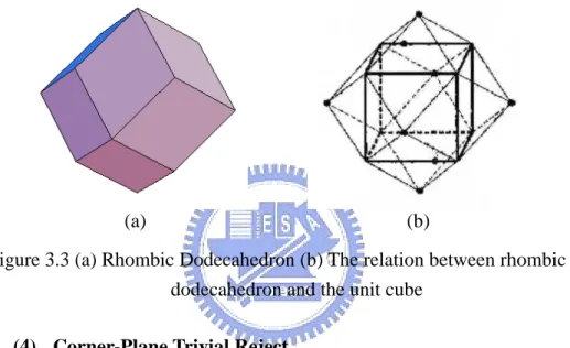
(3) Edge-Plane Trivial Reject

We compare the vertices of the model against the twelve planes

which touch the twelve edges of the cube. And these planes are at 45

degrees to their adjacent faces. This enclosed volume is a rhombic

dodecahedron, as shown in Figure 3.3. If all vertices are outside the

rhombic dodecahedron, this cube does not intersect the model.

Figure 3.3 (a) Rhombic Dodecahedron (b) The relation between rhombic dodecahedron and the unit cube

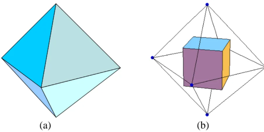
(4) Corner-Plane Trivial Reject

We compare the vertices of all triangles against the eight planes

that pass through one of the cube corners. These planes are

perpendicular to the corresponding diagonal of the cube. This enclosed

volume is octahedron, as shown in Figure 3.4. This cube does not

intersect the model if the vertices which belong to the model are

outside the octahedron

Figure 3.4 (a) Octahedron (b) The relation between octahedron and the unit cube

2. Second Phase

(5) Triangle Edges VS. Cube

We check if any triangles of the model penetrate the cube in the

second phase. We examine the relations between each edge of the

triangles and six faces of the unit cube. If any edge penetrates it, the

cube intersects the model.

3. Third Phase

(6) Cube Diagonals VS. Triangle

We check whether a cube corner pokes through the interior of the

triangle by examining the relations between four cube diagonals and the

triangle. We can obtain four intersection points which belong to

diagonal lines and the plane which includes the triangle. Four corners of

the cube do not poke through the triangle when the points are not inside

the cube. However, if anyone is inside, we should further examine

whether the point is inside the triangle. We use three cross products

whose vectors belong to the point and the vertices of the triangle to

check this point, as shown in Figure 3.5. The corner pokes through the

interior of the triangle if three vectors have the same direction. Then the

cube intersects the model.

4. Remaining

Finally, there are some remainding cubes which do not belong to any

cases as mentioned before. These cubes do not intersect the model.

Figure 3.5 Three cross products of the conditional check

3.1.2 Correction of Polycube Structure

A polycube of the model has been constructed using the triangle-cube

intersection algorithm [6]. The model is inside the polycube. However, some textures

which are tiled on the surfaces of the polycube can not be mapped on the model

because some unit cells that are converted from unit cubes do not intersect the model.

The followings describe the three properties of unit cells:

1. Each cell equals in size to a unit cube. ：The intersection point

2. Each cell is centered in a corner of the unit cubes.

3. Each cell intersects the polycube.

An example is shown in Figures 3.6 and 3.7. There are non-consecutive textures

on the model by mapping with this polycube. In this section, we will detect

non-intersectional cells and remove them to modify the structure of the polycube

before tiling textures.

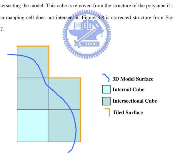
At first, we trace each intersectional cube of the polycube, as shown in Figure

3.6. For each cube, we should examine eight cells converted from the cube if they are

intersecting the model. This cube is removed from the structure of the polycube if any

non-mapping cell does not intersect it. Figure 3.8 is corrected structure from Figure

3.7.

Figure 3.6 2D analogue: relation between polycube and 3D model

Internal Cube Intersectional Cube 3D Model Surface

As mentioned above, we construct the polycube of the 3D model by using the

triangle-cube intersection algorithm [6] and correct the structure of the polycube.

Finally, the model is not inside the polycube. They are intersecting with each other.

Figure 3.7 2D analogue: relation between cells mapping and 3D model

Figure 3.8 2D analogue: correction of the polycube structure

Cells of Polycube Mapping Direction Non-Mapping Cell Tile Un-Mapping On The Surface

3.2 Texture Tiling on Polycube

When the polycube has been produced, we extend the concept of Wang tiles [4]

to tile texture on the surfaces of the polycube. Our algorithm consists of two parts.

One is the edge coloring which arranges each square surface on the polycube

corresponding to four samples. The other is the tile construction which synthesizes

four samples to form a tile of each square surface. Finally, we accomplish a seamless

texture tiling on the surfaces of the polycube.

3.2.1 Edge Coloring

This algorithm is based on the approach of Fu and Leung [9]. At first, there are

four diamond samples randomly selected from the input texture. Then we divide all

edges of the surfaces on the polycube into three groups, namely, X, Y, and Z,

according to three axial directions. An example is shown in Figure 3.9. For each

group, we randomly select two from four samples. Then each edge of the surface

corresponds to a sample which is randomly selected from its group samples.

Figure 3.9 Edge groups of the unit cube Unit

Cube

X-Axis Edge Y-Axis Edge Z-Axis Edge

In order to tile textures on the 3D polycube seamlessly, we slightly modify the

concept of Wang tiles [4] by rotating samples. An example is shown in Figure 3.10. A

sample is divided into upper and lower portions. When it is tiled on the surface of a

unit cube, the lower half is on the top side of the blue surface and the upper half is on

the right side of the yellow surface. We should appropriately rotate a sample 90

degrees counterclockwise for keeping up seamless tiling when tiling on the yellow

surface. Another example is shown in Figure 3.11. We should rotate a sample 90

degrees counterclockwise when tiling on the blue surface.

Figure 3.10 A unit cube with a tiled sample

Unit Cube

Right Surface Top Surface

Tiled Sample Rotated Sample

Figure 3.11 Three unit cubes with a tiled sample

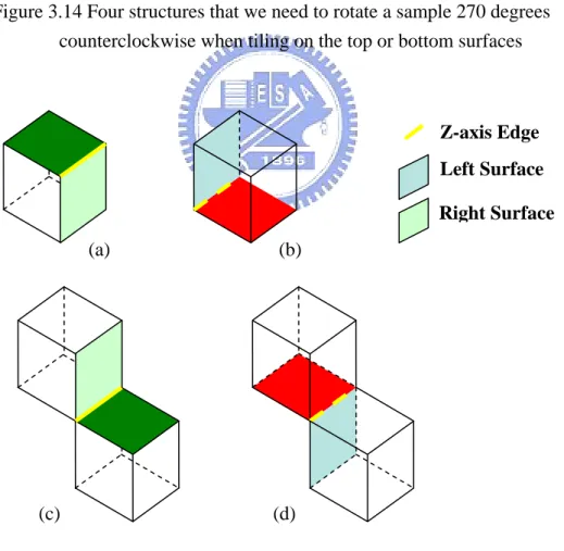
Therefore, we do not rotate samples when synthesizing tiles on the forward, left,

backward, and right surfaces, as shown in Figure 3.12. When we synthesize tiles on

the top and bottom surfaces, a sample which corresponds to the edge along X-axis

may be rotated 180 degrees, as shown in Figure 3.13. And a sample which

corresponds to the edge along Z-axis may be rotated 90 or 270 degrees

counterclockwise, as shown in Figures 3.14 and 3.15.

Therefore, each edge on the surface of the polycube corresponds to a suitable

sample. This sample may be rotated when tiled on the surface. We can tile textures on

the surface seamlessly by using this algorithm.

Right Surface on the Unit Cube A

A

B

Top Surface on the Unit Cube B

Figure 3.12 Expansion of the unit cube from Figure 3.9

Figure 3.13 Four structures that we need to rotate a sample 180 degrees when tiling on the top or bottom surfaces. (a), (b), (c), and (d) are the portions of the polycube.

Lef Forward Right Backward To Bottom Non-rotated Sample (a) (d) (b) (c) Bottom Surface X-axis Edge Backward Surface Unit Cube Top Surface

Figure 3.14 Four structures that we need to rotate a sample 270 degrees counterclockwise when tiling on the top or bottom surfaces

Figure 3.15 Four structures that we need to rotate a sample 90 degrees counterclockwise when tiling on the top or bottom surfaces.

Z-axis Edge Right Surface Left Surface (d) (c) (b) (a) Z-axis Edge Right Surface Left Surface (d) (c) (b) (a)

3.2.2 Tile Construction

In this section, our system will tile textures on each square surface of the

polycube by using the method based on the approach of Cohen et al. [4]. A user can

choose image quilting [7] or graph cuts [21] algorithms to synthesize a tile from four

diamond samples which correspond to the edge of the square surface.

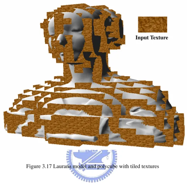
Finally, we accomplish seamless texture tiling on the surface of the polycube. A

result is shown in Figures 3.16 and 3.17

Figure 3.17 Laurana model and polycube with tiled textures

Chapter 4

Generation of Texture Mapping

In this chapter, we discuss how to generate rectangular cells which are

transformed from the polycube and map textures onto the model. Our concept is based

on polycube-maps [20]. In Section 4.1, we describe the generation of cells. In Section

4.2, some cells which intersect the model can not map any textures on the model. We

construct rectangular cells to solve this problem. Then we accomplish cells mapping

from the textures on the polycube to the model in section 4.3.

4.1 Transforming Polycubes to Polycells

In order to reduce mapping distortion, we apply cells mapping which is based on

polycube-maps [20]. Our algorithm defines mapping directions according to the

configuration inside a cell. Therefore, we need to transform the polycube to the

polycell which consists of unit cells before mapping textures onto the model. We can

easily construct the polycell by the properties as mentioned in Section 3.1.2. An

Figure 4.1 2D analogue: relation between the polycube and the polycell

We further create the configurations inside external cells which intersect the

portions of the tiles on the surfaces. We consider the intersection between external

cells and the tiles on the polycube. Each tile is subdivided into four slices. An

example is shown in Figure 4.2. There are 63 different configurations of the slices

inside a cell. If we remove rotational and reflectional similarities, these configurations

can be further reduced to six basic configurations, as shown in Figure 4.3.

Finally, we construct the polycell and the configurations inside each cell. There

are some advantages：

1. It is easy to determine the vertices of the polycell.

2. The number of the configurations inside the cells is limited to six because

the similarities of rotations and reflections are removed.

3. These basic configurations have different mapping functions. Each function

Cells of Polycube

Tiles on the Surfaces Unit Cubes

is related to the structure of the tiles on the polycube so that we can reduce

the distortion when mapping on the model.

Figure 4.2 2D analogue: relation between the polycube and the polycell

4.2 Rectangular Cells Construction

From Section 3.1.2, we know that all external cells intersect with the model

surface. We will process each external cell to map textures on the model. However,

we detect a few internal cells which intersect the model, but the configurations inside

these cells are empty. A reason is that the polycube can not approximate the curvature

of the model surface exactly. An example is shown in Figure 4.4. These internal cells,

grouped in set Κ, can not map any textures and cause gaps on the model.

Unit Cubes Internal Cells

Configurations of Tile Slices inside the Cells

Figure 4.3 Six basic configurations

In order to solve this problem, we combine each internal cell of Κ with an

external cell which is adjacent to it. At first, adjacent external cells for each internal

cell are numbered and processed from small to large. The purpose of this algorithm

avoids an internal cell merging none of the external cell.

Then we examine six surfaces of the internal cell which intersects the model by

using the triangle-cube intersection algorithm [6]. If only one surface intersects, we

merge two cells which include this surface together. Figure 4.5 shows the

modification of Figure 4.4. If more than one surface intersects, we choose an external

cell whose configuration map is with lower distortion. Type4b has the lowest

distortion in all configurations. Our priority for selection from high to low is Type 4b,

Type 4a, Type 3, and Type 5. A resulting example is shown in Figure 4.6 and 4.7.

Type 6a and Type 6b are impossible adjacent to the internal cell in Κ because all

Type 3 Type 4a Type 4b

surfaces of the cells are connected the slices. Therefore, we do not apply these two

configurations in rectangular cells.

Figure 4.4 2D analogue: an internal cell intersects the model but is empty

Therefore, we solve the empty problem in the internal cells of Κ by using

rectangular cells. However, some of rectangular cells may create seams on the model.

There are two reasons of the problem:

1. The size of a unit cell is too large.

2. The curvature of the model is too high.

Figure 4.8 shows an example of this problem. We can reduce the size of the unit

cube to decrease the appearance of the seams but can not promise to avoid this

problem completely. Internal Cells Intersecting the Model Internal Cube Intersectional Cube Tiled Surface External Cells 3D Model Surface

Figure 4.5 2D analogue: combination of internal and external cells

Figure 4.6 2D analogue: two surfaces of the internal cell intersects the model

Internal Cell 3D Model Surface

Figure 4.7 2D analogue: combination of internal and external cells

Figure 4.8 2D analogue: combination of internal and external cells

Rectangular Cell Mapping Direction

Portion of Wrong Mapping

4.3 Cells Mapping

In this section, we describe the mapping functions of six configurations and how

to map the textures onto the model. We process each triangle of the model separately

and subdivide it into several slices according to the intersectional cells. Each slice is

included only one cell. Then we apply cells mapping to map the textures onto the slice

inside the cell.

Figure 4.9 Mapping directions of six basic configurations

4.3.1 Mapping Function of Cell Configurations

As mentioned in Section 4.1, we know that all different configurations in the

polycell could be reduced to six basic cases. In this subsection, we define mapping

directions of the basic configurations which are based on polycube-maps [20], as

Type 3 Type 4a Type 4b

shown in Figure 4.9. In Section 4.2, we increase four rectangular configurations to

process the internal cells in Κ. Figure 4.10 shows all mapping directions of

rectangular configurations. Table 4.1 shows the mapping functions of other

configurations.

Table 4.1 Mapping functions of six configurations

Configuration Mapping Directive Vector

Type 3 (r, s, t) Type 4 (r, s, 0) Type 4b (0, 1, 0) Type 5 r t if t s r t r _{− − − ≥} ), 1 , 1 , ( r t if t r t s r − − < − ,1 , ), 1 ( Type 6a (1-r, 1-s, 1-t) Type 6b r t if t s r t r _{− − − ≥} ), 1 , 1 , ( 1 , ), , , 1 ( − −s t if t <r t+s< s t r 1 , ), 1 , , 1 ( −r s −t if t<r t+s> r t s Coordinate Axis

Figure 4.10 Rectangular mapping directions of four configurations, (a), (b) and (c) are Type 3, (d) and (f) are Type 4a, (e) is Type 4b,and (g) is Type 5

(a) (b)

(c) (d) (e)

(f)

4.3.2 Texture Mapping on Model

In this subsection, we process triangles of the model separately to map textures.

At first, we search the cells which intersect the bounding box of a triangle. Then we

consider the intersection between these cells and a triangle. If a triangle is inside one

cell completely, we use the mapping function of the cell to map textures onto it. If not,

we need to acquire the intersectional points by detecting a triangle with the cells.

There are two kinds of points between a triangle and a cell described as follows:

1. Three edges of a triangle and six surfaces of a cell

2. Twelve edges of a cell and the interior of a triangle

Figure 4.11 A triangle is subdivided into four slices by a cell

Some intersectional points are increased in the triangle. A triangle is subdivided

into several slices by cells and each slice is included in a cell. An example is shown in

Figure 4.11. Then we separately process each slice to map textures onto it according

to the mapping function of the cell which includes it.

An interior point of a triangle A point in the edge of a triangle

Four slices of a triangle

Finally, we accomplish to map textures of the polycube onto the slices which

Chapter 5

Implementation and Results

In this chapter, we demonstrate our implementation results. The input sources are

a texture and a 3D model. Our algorithm are implemented in C# language on VC.Net

with a Pentium4 3.4GHz PC with 2 GB memory.

(a) (b)

Figure 5.1 (a) example 1: an input texture and (b) a laruana model

An input example with a 183x100 texture image and a laurana model are shown

in Figure 5.1. An intermediate result is the polycube of the model with unit cubes, as

shown in Figure 5.2(a). Figure 5.2(b) shows that the relation between the polycube

and the model. They are intersecting with each other. Figure 5.2(c) shows the

polycube with tiled textures and Figure 5.2(d) shows that an image is enlarged from Example 1

the yellow region in Figure 5.2(c). Each tile is combined by graph cuts algorithm. The

final result is shown in Figure 5.3. And Figure 5.5 shows another result with different

texture sample.

(a) (b)

(c)

Figure 5.2 (a) a polycube of the laruana model, (b) relation between the polycube and the model, (c) polycube with the tiled textures and (d) an enlarged image

(b)

(c)

Figure 5.3 (a) Textures map onto the model, (b) and (c) are enlarged images form the portions of (a)

Figure 5.4 shows a result of Fu and Leung [9]. Table 5.1 shows the comparison

with our result.

Table 5.1 Comparison between our result and Fu and Leung [9]

Our algorithm Fu and Leung [9]

Size of a unit cube Small Large

Number of unit cubes Many Few

Size of patterns Small Large

(b)

Figure 5.4 (a) a polycube of the laruana model [20] (b) a result of the laruana model in Fu and Leung [9]

(b)

(c)

Figure 5.5 A mapping result with the texture example 2, (b) and (c) are enlarged images

Example 2

Table 5.2 shows the information of Figure 5.3 and 5.5.

Table 5.2 Information during texture mapping by using different examples

Model Laruana

Input texture Example 1 Example 2

Size of the input texture 183x100

Size of a tile 32x32

Number of unit cubes 2555

Number of surfaces on the polycube

4264

Number of different tiles 804 800

Time of constructing the polycube with tiles

5 min. 03 sec. 5 min. 09 sec.

Time of mapping from the polycube to the model

33 sec. 33 sec.

Figure 5.6 shows a synthesized texture by Wang tiles [4]. Figure 5.7 and 5.8

show that the results are mapped with the same input texture but different size of the

unit cubes. Example 3 is our input texture and a 400x400 image. Figure 5.8 has lower

distortion than Figure 5.7. But the size of

patterns in Figure 5.8 is smaller. We can

not avoid some unconnected regions, as

compared with Figure 5.6 (b).

Figure 5.6 (a) an input in Wang tiles (b) A synthesized texture from (a) [4]

(b) (a)

(b)

Figure 5.7 A mapping result with the texture example 3 and (b) and (c) are enlarged images

(c) (a) ( )

(b)

(c)

Figure 5.8 A mapping result with the texture example 2 and (b) and (c) are enlarged images

Table 5.3 Information during texture mapping by using dixfferent sizes of unit cubes

Model Laruana

Input texture Example 3

Size of the input texture 400x400

Size of a tile 64x64

Size of a unit cube 25:21

Number of unit cubes 2555 3657

Number of surfaces on the polycube

4264 6030

Number of different tiles 766 940

Time of constructing the polycube with tiles

8 min. 18 sec. 10 min. 40 sec.

Time of mapping from the polycube to the model

30 sec. 47 sec.

Another input model is a teapot, as shown in Figure 5.9(a), and an input texture

is example 2. Figure 5.9(b) shows the polycube of the teapot with tiled textures. The

final result is shown in Figure5.10.

(b)

Figure 5.9 (a) A teapot model (b) The polycube of teapot with tiled textures

(b)

(a)

(c)

Figure 5.10 A mapping result with the texture example 2 and (b) and (c) are enlarged images

Example 4 is a 128x128 image, as shown in Figure 5.11. We apply different sizes

of a tile. The final result is shown in Figure5.12. And the corresponding information

about the teapot model is shown in Table 5.4.

Figure 5.11 Example 4: an input texture

Table 5.4 Information during texture mapping by using different input textures

Model Teapot

Input texture Example 2 Example 4

Size of the input texture 183x100 128x128

Size of a tile 32x32 64x64

Number of unit cubes 1425

Number of surfaces on the polycube

2568

Number of different tiles 648 679

Time of constructing the polycube with tiles

3 min. 56 sec. 8 min 35 sec.

Time of mapping from the polycube to the model

(b)

(a)

(c)

Figure 5.12 A mapping result with the texture example 4 and (b) and (c) are enlarged images

An input example with a 433x640 texture image and a Daba model are shown in

Figure 5.13. Figure 5.14 shows the polycube of the model with tiled textures. And

final result is shown in Figure 5.15.

(a) (b)

Figure 5.13 (a) a Daba model and (b) example 5: an input texture

(a)

(b) (c)

(a)

(b) (c)

Figure 5.16 and 5.17 show the results with texture Example 2 and 6. The

corresponding information about the Daba model is shown in Table 5.5.

(b)

(c) (d)

Figure 5.17 (a) Example 6: A 200x200 input texture (b) A mapping result with the texture example 6 and (c) and (d) are enlarged portions

Table 5.5 Information during texture mapping by using different input textures

Model Daba

Input texture Example 5 Example 2 Example6

Size of the input texture 433x640 183x100 200x200

Size of a tile 64x64 48x48 64x64

Number of unit cubes 1798

Number of surfaces on the polycube

2730

Number of different tiles 541 561 566

Time of constructing the polycube with tiles

6 min. 15 sec. 5 min 55 sec. 6 min. 13 sec.

Time of mapping from the polycube to the model

27 sec. 31 sec. 28 sec.

There are few apparent distortions in our results. These distortions are usually

formed by the configurations of Type 5, Type 3 and Type 6. If we decrease the size of

a unit cube, the shape of the polycube is close to the model. Then we reduce the

distortions on the model. However, the size of patterns is reduced together. We can

decrease the size of a tile so that the size of patterns is enlarged. However, the size of

Chapter 6

Conclusions

In this thesis, we proposed a method to map texture on 3D models automatically.

The proposed approach consists of two important processes: polycube construction

and cells mapping. In the first process, we use the triangle-cube intersection algorithm

[6] to construct the polycube of a model. Then we tile texture on the polycube

seamlessly. Second, we process cells of the polycell separately. The textures of the

cell are mappe d on the model according to its mapping direction. Therefore, users

may generate texture mapping on the model by using our system easily. Table 6.1

shows the differences between our system and polycube-maps [20].

However, there are still some issues in our system.

1. Our system is not generic for some models which have a portion with large

curvature, such as the ear of the bunny model.

2. In our experiment, we found that some cubes intersect only few regions of

the model. The textures are compressed seriously when mapping them on

Table 6.1 Differences between two methods

Our algorithm Polycube-maps

Polycube construction Automatic

Warping Polycube No

User intervention

Extra time No Yes

Inverse warping No Yes

Size of a unit cube Small Big

Number of unit cubes Many Few

In order to solve these problems, we reduce the size of a unit cube so that the

shape of the polycube is close to the model. The distortion and the size of patterns on

the model are reduced simultaneously. There is a trade-off between the distortion and

the size of patterns on the model.

In the future, we will use different size of the unit cubes to construct the

polycube. The shape of the polycube is similar to the model. Not all size of the square

surfaces on the polycube is reduced. We can reduce the distortion and maintain the

size of patterns at the same time. Another method of inverse warping can be used to

reduce the distortion. We estimate the distortion of the cells before mapping on the

model. The texture is warped in advance. Then we obtain the better results with the

Reference

[1] Alan, W., 2000. 3D computer graphics. 3rd Ed., Addison Wesley, pp.245-247

[2] Carr, N. A., AND Hart, J. C. 2002. Meshed atlases for real-time procedural solid texturing. ACM Transactions on Graphics 21, 2, 106–131.

[3] Cignoni, P., Montani, C., Rocchini, C., Scopigno, R., AND Tarini, M. 1999. Preserving attribute values on simplified meshes by resampling detail textures. The Visual Computer 15, 10, 519–539.

[4] Cohen, M. F., Shade, J., Hiller, S., AND Deussen, O. 2003. Wang tiles for image and texture generation. ACM Transactions on Graphics 22, 3, 287–294.

[5] Culik II, K. 1996. An aperiodic set of 13 Wang tiles. Discrete Mathematics 160, 245–251.

[6] Douglas, V. 1992. Triangle-cube intersection. Graphics Gems III, pp. 236-239

[7] Efros, A., AND Freeman, W. 2001. Image quilting for texture synthesis and transfer. In Proceedings of SIGGRAPH 2001, 341–346.

[8] Efros, A., AND Leung, T. 1999. Texture synthesis by non-parametric sampling. ICCV, 1033-1038.

[9] Fu, C. W., AND Leung, M. K., 2005. Texture tiling on arbitrary topological surfaces. Proceedings of Eurographics Symposium on Rendering, 99-104, [10] Grünbaum, B., AND Shephard, G. C. 1986. Tilings and patterns. W. H.

Freeman and Company. ISSN 0716711931.

[11] Grimm, C. M. 2002. Simple manifolds for surface modeling and parameterization. In Proceedings of Shape Modeling International 2002, 237–244.

[12] Hertzmann, A., Jacobs, C., Oliver, N., Curless, B., AND Salesin, D. 2001. Image analogies. ACM SIGGRAPH, 327-340.

[13] Lévy, B., Petitjean, S., Ray, N., AND Maillot, J. 2002. Least squares conformal maps for automatic texture atlas generation. ACM Transactions on Graphics 21, 3, 362–371.

[14] Maillot, J., Yahia, H., AND Verroust, A. 1993. Interactive texture mapping. In Proceedings of ACM SIGGRAPH 93, 27–34.

[15] Piponi, D., AND Borshukov, G. 2000. Seamless texture mapping of subdivision surfaces by model pelting and texture blending. In Proceedings of ACM SIGGRAPH 2000, 471–478.

[16] Sander, P., Wood, Z., Gortler, S. J., Snyner, J., AND Hoppe H. 2003. Multi-chart geometry images. In Proc. of the Symposium on Geometry Processing 2003, 146–155.

[17] Sheffer, A., AND Hart, J. C. 2002. Seamster: inconspicuous low distortion texture seam layout. In Proceedings of Visualization 2002, 291–298.

[18] Sorkine, O., Cohen-or, D., Goldenthal, R., AND Lischinski, D. 2002. Bounded-distortion piecewise mesh parameterization. In Proceedings of Visualization 2002, 355–362.

[19] Stam, J., 1997. Aperiodic texture mapping. Tech. rep., R046. European Research Consortium for Informatics and Mathematics (ERCIM). http://www.ercim.org/publication/technical reports/046-abstract.html.

[20] Tarini M., Hormann K., Cignoni P., Montani C., 2004. Polycube-maps. In Proceedings of SIGGRAPH 2004, 853–860.

[21] Kwatra, V., Schodl, A., Essa, I., Turk, G., AND Bobicks, A. 2003. Graphcut textures: image and video synthesis using graph cuts. In Proceedings of ACM SIGGRAPH , pp.277-286.

[22] Wang, H. 1965. Games, logic, and computers. Scientific American (November), 98–106.

[23] Wang, H. 1961. Proving theorems by pattern recognition ii. Bell Systems Technical Journal 40, 1–42.

[24] Wei, L. Y., AND Levoy, M. 2000. Fast texture synthesis using tree-structured vector quantization. ACM SIGGRAPH, 479-488.