國 立 交 通 大 學
電信工程研究所
博 士 論 文
波束掃瞄天線及平面反射天線創新研究
New Beam-steering Antennas and Planar
Reflector Antennas
研 究 生:譚怡陽
指導教授:鍾世忠
國 立 交 通 大 學
電信工程研究所
博 士 論 文
波束掃瞄天線及平面反射天線創新研究
New Beam-steering Antennas and Planar
Reflector Antennas
研 究 生:譚怡陽
指導教授:鍾世忠
波束掃瞄天線及平面反射天線創新研究
New Beam-steering Antennas and Planar
Reflector Antennas
研 究 生:譚怡陽 Student:I-Young Tarn
指導教授:鍾世忠博士 Advisor:Dr. Shyh-Jong Chung
國 立 交 通 大 學
電信工程研究所
博 士 論 文
A Dissertation
Submitted to the College of Electrical Engineering and
Computer Science, National Chiao Tung University
in Conformation with the Requirements for the Degree of
Doctor of Philosophy
Accepted by the Department of Communication Engineering
March 2008
Hsinchu, Taiwan, Republic of China
中文摘要
本論文以新的天線波束掃瞄技術和平面式反射天線為主軸,深入探討五個 題目。首先是一個具波束掃描功能之波導饋入微帶天線陣列,藉由小幅度改變波 導管厚度造成傳播常數變化,控制饋送到每個天線元之間的相位差,因而使得天 線陣列的波束方向偏轉。 第二個是雷達和通訊雙模的平面摺疊式反射陣列天線,由於次反射面的作 用,此天線操作在雷達模態時電磁波會經由主反射面聚焦,產生可切換方向的窄 波束,而通訊模態則呈現寬波束的輻射場型,兩種模態的場型各有其適合的應用。 此外,本文也對毫米波圓極化選擇性表面加以研究,在用印刷電路技術實 現第一種形式的圓極化選擇性表面後,發現連通電路板兩面的垂直方向金屬孔在 製作時會衍生一些非預期效應,進而影響到圓極化選擇的特性,因此發展出另一 種設完全沒有垂直方向導體的三層純平面式圓極化選擇性表面,第二種設計以電 磁耦合取代導體直接相連,可省去製作大量金屬連通孔的困擾,更適用於印刷電 路的製程。 最後,研究出使用最少數量微波開關元件即可控制大範圍頻率選擇性表面 的方法,並與角反射天線的概念結合,完成一個創新的輻射場型分集天線,此天 線在不同的開關狀態組合情況下各有相對應的波束方向和輻射場型。 本論文中所有的研究,都是先建構好工作原理,然後經由計算和模擬找出 最佳化設計,成品的實際量測數據和模擬結果皆相當吻合。各項成果已達預期效 果,未來可以繼續個別的研究增強性能,更可進一步相互搭配結合,創造出更多 樣的功能及應用。Abstract
This dissertation deals with novel beam steering techniques and planar reflector antennas. A beam-steering waveguide-fed microstrip antenna array, a dual-mode millimeter-wave folded microstrip reflectarray antenna, a millimeter-wave right-hand circular polarization selective surface, a millimeter-wave three-layered left-hand circular polarization selective surface without any vertical conductive segment and a pattern diversity reflector antenna with minimum number of switching devices have been investigated, designed, built and tested. The theoretical approaches and practical developments of the above five researches are comprehensively discussed. All the simulated results are verified experimentally, and exhibit good consistency with the measured data. The individual subjects are worth further efforts for improvements in the future. Moreover, it is advisable to deploying new applications by combining some of the researches presented in this dissertation.
致謝
原本一直以為我的學生生涯已經結束,從沒想到過八年前竟然還能得到機 會,進入博士班研讀,為此,我滿懷珍惜與自勉,迎向這個挑戰和磨練。而今終 於邁向尾聲,整個過程,遠比我想像中的漫長許多許多。上課、考試、資格考、 想題目、設計、製作、量測、投稿、一再修稿……每每以為克服這關,下關就容 易了,現在知道其實不然,沒有一件事可以輕鬆得了的。就在即將完成畢業論文 的此刻,卻忽然發現連誌謝也不好寫,想了很久,才慢慢理出一點思緒。 在博士班求學的過程中,首先感激我的指導老師鍾世忠教授,能夠容忍我 這麼個不專業的學生。由於在職的緣故,我沒有像實驗室其他人一樣和老師有頻 繁的互動,大多是等達成一定程度的進展後才敢找老師報告,而老師總能和顏悅 色地瞭解後,很快掌握住核心,然後提出可能的問題,建議繼續進行的方向,每 次討論結束後都夠我又忙好一陣子。老師的指導除了讓我做論文時獲益良多,條 理清晰的思考方式和研究精神才更值得效法。 剛入學時,幾乎每天掛念著課業和資格考,日子過得很緊張,幸有同為在 職的博士班同學饒瑞榮能夠一起討論,給了我許多幫助。實驗室歷屆的學弟學妹 們,尤其是尤寶樺、梅家豪、李彥璋、陳星銘、林融聖、邱建評、羅文信、柯智 祥、王侑信、凌菁偉、何丹雄、饒佩宗、林靖凱等幾位,在我做論文時也給我很 大的影響。有時在實驗室留到很晚,不管是探討研究相關的議題或單純只是閒 聊,離開時即使已經相當疲憊,心情卻充實又愉悅,偶爾甚至有點振奮的感覺, 這種在職場上難有的體會,格外令人回味。祝福大家各自擁有錦繡前程,更期待 將來有機會可以彼此相互拉拔扶持。 是學習、更像是磨練,追求知識長進雖有些許成績,然而這次的進修同時 也讓劣根性逐一顯露,變得越來越不懂寬容和體諒,忘了樂觀,忘了應有的關懷, 更忘了什麼叫珍惜。我的摯友,讓我有了希望和夢想,不斷鼓舞著我,在我低落時總會使我再度產生勇氣,給我心靈最穩定的力量。我的家人,默默地支持我, 任何時候都會做我最溫暖而堅強的後盾。感到挫折或不滿時,每念及此,就會覺 得自己何其有幸,不該有太多的埋怨。但願我能記取教訓,有所領悟,今後能常 提醒自己鍛鍊得更加勇敢、沉穩、智慧、和為人著想。雅彩、雅梅、伯父、伯母, 想了很久還是發現,無論怎樣都難以完整表達我的感激,但所有一切我將永遠銘 記在心。Data 和 Teng,謝謝你們不時的關心,而且為了幫我修論文竟然連幾天 熬夜,實在過意不去。宜珮,謝謝你的付出和擔待,以及你們一家人對我的包含 和照顧。爸、媽,別再偷偷為我操煩了。眾人的高情厚誼,是最豐盛又無可取代 的寶藏,我也期許自己在各方面繼續努力,有一天讓大家感到欣慰和榮耀。
Contents
中文摘要... iii
Abstract...iv
致謝...v
1 Introduction...1
2 A Beam-Steering Waveguide-Fed Microstrip Antenna Array ...1
2.1 Introduction...1
2.2 Theory...1
2.3 Design ...3
2.3.1 Series-Fed Microstrip Antenna Sub-Array ...5
2.3.2 Coupling from Rectangular Waveguide to Microstrip Line ...8
2.3.3 Waveguide-fed Antenna Array...8
2.4 Measurement Results...11
2.5 Conclusions...11
References...15
3 A Dual-Mode Millimeter-Wave Folded Microstrip Reflectarray Antenna ...16
3.1 Introduction...16 3.2 Principle ...17 3.3 Design ...22 3.3.1 Feed Antenna ...23 3.3.2 Sub-reflector ...26 3.3.3 Main Reflector ...27
3.3.4 Beam Switching Mechanism ...35
3.4.1 Radar Mode...39
3.4.2 Communication Mode ...44
3.5 Conclusions...51
References...52
4 A 60 GHz Circular Polarization Selective Surface by Printed Circuit Technology 54 4.1 Introduction...54 4.2 Operational Principle ...55 4.3 Analysis Method ...58 4.4 Results...59 4.5 Conclusions...69 References...71
5 A New Advance in Circular Polarization Selective Surface – A Three Layered CPSS without Vertical Conductive Segments...73
5.1 Introduction...73 5.2 Principle ...77 5.3 Design ...87 5.4 Measurement...97 5.5 Conclusions...104 References...110
6 A Novel Pattern Diversity Reflector Antenna Using Reconfigurable Frequency Selective Surfaces ... 111
6.1 Introduction... 111
6.2 Design ...113
6.2.1 Feed Antenna ...114
6.2.3 Novel Reconfigurable FSS Design ...115
6.3 Results...123
6.4 Conclusions...133
References...134
7 Conclusions and Future Works ...137
Vita...142
List of Figures and Tables
Figure 2.1 Schematic diagram of a waveguide-fed microstrip antenna array. ...2
Figure 2.2 Photograph of the microstrip antenna array. ...4
Figure 2.3 The photograph of the finished series-fed sub-array...6
Figure 2.4 The equivalent circuit of a series fed microstrip array. ...7
Figure 2.5 The measured and calculated coupling coefficients as functions of the length of microstrip open-end...9
Figure 2.6 Return loss of the waveguide-fed microstrip antenna array...13
Figure 2.7 Comparison of the H-plane patterns of the waveguide-fed microstrip antenna array at 37.8 GHz. ...14
Figure 3.1 The schematic diagram of the proposed folded reflectarray antenna...19
Figure 3.2 Coordinates for the analysis of the folded reflectarray antenna...21
Figure 3.3 The measured radiation patterns of the feed antenna at 38.5 GHz. ...25
Figure 3.4 Calculated aperture efficiency, as a function of the aperture’s diameter D of the folded reflectarray antenna...30
Figure 3.5 The field twisting effect of the 45° tilted square patch antenna with two open stubs...32
Figure 3.6 Calculated H-plane patterns of the folded reflectarray antenna for various Df at 38.5 GHz. ...34
Figure 3.7 Calculated H-plane patterns of the folded reflectarray antenna for various displacements (d) of the feed position at 38.5 GHz...37
Figure 3.8 Bottom view (left) and top view (right) of the sliding track mechanism, which is mounted with the main reflector...38 Figure 3.9 The measured H-plane patterns for various feed positions (d) at 38.5 GHz.
...40 Figure 3.10 Photo of the finished folded reflectarray antenna. ...41 Figure 3.11 The measured return losses of the fabricated folded reflectarray antenna
for d= 0 mm feed in the radar mode, and the single feed patch. ...42 Figure 3.12 The radar mode H-plane patterns of the folded reflectarray antenna at 38.5 GHz for various feed positions (d)...43 Figure 3.13 Four communication mode feed antennas: (a) The original feed patch
described in section 3.3. (b) The original feed patch enclosed with a metal ring trace. The width of the trace (w) is 3 mm and the radius of the ring (r) is 4.5 mm. (c) The original feed patch enclosed with a larger metal ring trace. Both the width of the trace (w) and the radius of the ring (r) are 6 mm. (d) The original feed patch enclosed by a metal square frame, with the trace width being 2.7 mm and the gap being 1 mm...46 Figure 3.14 The measured patterns for various feed antennas presented in Figure 3.13, with the sub-reflector removed. ...47 Figure 3.15 The measured cross-polarization patterns for various feed antennas
presented in Figure 3.13, with the sub-reflector removed. ...48 Figure 3.16 The measured communication mode input reflection coefficients of the
fabricated folded reflectarray antenna, for various feed antennas presented in Figure 3.13. ...49 Figure 3.17 The measured patterns at 38.5 GHz, with sub-reflector, for: (a) original
feed patch (Figure 3.13(a)), (b) original feed patch enclosed by a metal square frame (Figure 3.13(d)). ...50 Figure 4.1 Schematic of the CPSS. The constituent structure is a bent wire formed
with three jointed orthogonal segments. The total length of the whole wire is about 1λ. ...57
Figure 4.2 The 3×3 array used for analysis. The currents on the center unit cell are extracted for succeeding manipulations...60 Figure 4.3 The simulated isolation for various lengths of arms. The radii (r) of the
vias are 2 mils and 4 mils, respectively. ...62 Figure 4.4 The simulated transmission loss for various lengths of arms. The radii (r) of the vias are 2 mils and 4 mils, respectively...63 Figure 4.5 Photograph of the finished RHCPSS, which has 1256 elements on a
disk-shape substrate. The radius of the disk is about 45 mm...65 Figure 4.6 The simulated isolations for outer radius (r) of 0.1 mm, 0.15 mm and 0.2
mm (arm length l= 1.5 mm, inner radius= 0.075 mm), and the measured isolation of
the finished RHCPSS...66 Figure 4.7 The simulated transmission loss for outer radius (r) of 0.1 mm, 0.15 mm and 0.2 mm (arm length l= 1.5 mm, inner radius= 0.075 mm), and the measured data of the finished RHCPSS...67 Figure 5.1 (a) The constituent element of the CPSS structure proposed in [6]. (b) The constituent element of the CPSS structure proposed in [7]. ...75 Figure 5.2 (a) The unit cell of a CPSS that contains two perpendicular dipoles on top
and bottom layers and an L-shaped trace in the middle. (b) Top view of the unit cell...79 Figure 5.3 Isolations as a function of frequency for a unit cell with two perpendicular
dipoles located respectively on top and bottom layer of a 62-mil Duroid 5870 laminate (l=3.61 mm, periodicity= 4.5 mm)...82 Figure 5.4 Coupling factors as a function of frequency for the configuration shown in Figure 5.2 (l=3.61 mm. Periodicity= 4.5 mm)...84 Figure 5.5 The current directions on the upper and the lower dipoles excited by (a)
Figure 5.6 The current directions on the upper and the lower dipoles exited by (a) 27 GHz x-polarized plane waves, and (b) 27 GHz y-polarized plane waves. The dashed line indicates the couple currents...86 Figure 5.7 The simulated isolations as a function of frequency for the configuration
shown in Figure 5.2 (l= 3.61 mm, periodicity= 4.5 mm). ...90 Figure 5.8 (a) The schema of the proposed LHCPSS configuration. (b) Top view of a
unit cell of the LHCPSS, three L-shaped traces are implemented in the middle layer...91 Figure 5.9 Isolations at 30 GHz for various εr and thicknesses of the glue layer (p = 4 mm, l= 3.25 mm, l1= 3.295 mm, l2= 2.7 mm and l3= 2.3 mm). ...93
Figure 5.10 Transmission losses at 30 GHz for various εr and thicknesses of the glue
layer (p = 4 mm, l= 3.25 mm, l1= 3.295 mm, l2= 2.7 mm and l3= 2.3 mm). ...94
Figure 5.11 (a) Simulated isolations for several geometrical variables (l1, l3, p) with
respect to l. (b) Simulated transmission losses for several geometrical variables (l1, l3, p) with respect to l. ...96
Figure 5.12 (a) Normalized induced current on the metallic traces of the optimized LHCPSS illuminated with (a) LHCP wave, (b) RHCP wave. ...99 Figure 5.13 Photograph of the finished LHCPSS, with 185 elements on a disk-shape
substrate. The radius of the disk is about 55 mm...100 Figure 5.14 Schematic of the measurement setup. ...101 Figure 5.15 Picture taken during measurements. Two LP horn antennas are placed
about 60 cm apart, and the LHCPSS under test is put in the midst of them. ...103 Figure 5.16 The simulated and measured isolations for the LHCPSS of p = 6.25 mm,
l= 3.385 mm, l1= 2.9 mm, l2 = 3.0 mm and l3= 2.6 mm. ...106
Figure 5.17 The simulated and measured transmission losses for the LHCPSS of p = 6.25 mm, l= 3.385 mm, l1= 2.9 mm, l2 = 3.0 mm and l3= 2.6 mm. ...107
Figure 6.1 The geometry and parameters of the reconfigurable FSS. ...118 Figure 6.2 The equivalent circuit models of the reconfigurable FSS for (a) on-, and (b) off-state respectively. ...119 Figure 6.3 (a) The transmission coefficient curves for various widths of the loop in the
on-state. (b) The reflection coefficient curves for various widths of the loop in the off-state. ...121 Figure 6.4 An illustrative method of configuring a group of periodically distributed
microwave elements to the same state synchronously...122 Figure 6.5 The photograph of the finished pattern reconfigurable reflector antenna.
...124 Figure 6.6 The measured input return losses for the six cases of the pattern
reconfigurable reflector antenna as a function of frequency...126 Figure 6.7 The simulated and measured patterns of Case 1 at 2.45 GHz (a) for various azimuth cuts, and (b) in φ= 0o plane. ...127 Figure 6.8 The simulated and measured patterns of Case 2 at 2.45 GHz (a) for various azimuth cuts, and (b) in φ= 270o plane. ...128 Figure 6.9 The simulated and measured patterns of Case 3 at 2.45 GHz (a) for various azimuth cuts, and (b) in φ= 225o plane. ...129 Figure 6.10 The simulated and measured patterns of Case 4 at 2.45 GHz (a) for
various azimuth cuts, and (b) in φ= 0o plane...130 Figure 6.11 The simulated and measured patterns of Case 5 at 2.45 GHz (a) for
various azimuth cuts, and (b) in φ= 180o plane...131 Figure 6.12 The simulated and measured patterns of Case 6 at 2.45 GHz (a) for
various azimuth cuts, and (b) in φ= 0o plane...132 Figure 7.1 Schematic diagram of circular polarization folded reflectarray antenna. (a) Topology, (b) Phase compensation method. ...141
TABLE I The calculated coupling power and phase for each aperture in the
waveguide-fed array, and the associated aperture dimensions and open stub length. ...10 TABLE II The definitions of the six fundamental cases and their corresponding
1 Introduction
Generally, a microstrip reflectarray antenna consists of a flat array of patches or dipoles printed on a thin dielectric substrate. It works in a similar concept to a conventional reflector antenna, but without the bulky configuration and mechanical complexity. As compared to a phased array, the fields from the feed antenna are spatially fed to the individual elements on the array, and thus without suffering from high propagation losses in the intricate feeding network. Therefore, the reflectarray antenna combines the advantages of the reflector antenna and the phased array antenna.
For a folded reflectarray, the required depth is only half of that of a reflectarray antenna. This further reduces the antenna volume. In addition, unlike the conventional dual-reflectors antennas, the folded reflectarray antennas are free from the blocking effect of the sub-reflectors. The radiation beam can be steered by mechanically tilting the main reflector, or shifting the position of the feed antenna. By virtue of compactness, low loss, high gain, superior design flexibility, and the ease of manufacture, folded reflectarrays could be extensively used in wireless LAN, fixed wireless access, local to multi-points distribution service, satellite communications, short-haul personal communication networks, radar applications, and wireless intelligent transport systems.
In this dissertation, we proposed a new folded microstrip reflectarray antenna which can simultaneous operated in two modes. In the radar mode, the antenna demonstrates high gain and narrow beamwidth characteristics. The beam steering is performed by electrically switching the feed antennas. In the communication mode, the beamwidth is much broader and thus provides communications over a wide
angular range.
Currently, most folded reflectarrays are dedicated to linear polarization applications. With the emergency of excellent circular polarization selective surfaces, which can pass one sense of circularly polarized waves while reflecting the other, folded reflectarray could be extended to circular polarization applications. Therefore, we proposed a milli-meter wave circular polarization selective surface. It was realized by using printed circuit technology. Metal traces were created on both sides of a laminate, and connected by vertical conductive vias. This design performs well, yet implementing numerous, dense and thin vias accurately and stably is still hard to achieve at high frequencies.
To avoid the problems associated with the vertical conductive segments and increase flexibility in design motivated the drive to invent a new type of circular polarization selective surfaces that is composed of only transverse elements but no vias. The second circular polarization selective surface is a thoroughly stratified configuration with transverse planar elements implemented on different layers, and thus is well suited for multi-layered printed circuit board manufacturing process. This design has revolutionized the way in which the function of discriminating different circularly polarized waves is established. Connections between the elements on the top and bottom layers, which are built through the couplings caused by the intermediate part in the middle layer, make the blocking effect for different circularly polarized illuminations diverse.
Planar reflectors could be applied to radiation pattern diversity antennas as well. We designed and developed novel switchable frequency selective surfaces and used them to construct a corner reflector antenna. By configuring the states of the frequency selective surfaces, various beam patterns can be formed and steered in the
azimuth plane.
In addition, another beam steering antenna is presented in this dissertation. It is a waveguide-fed antenna, composed of series-fed microstrip patch arrays that are distributed along a straight line with fixed separations. The phase difference between two adjacent sub-arrays varies with the propagation constant, which can be controlled by changing the width of the feeding waveguide, and thus leads to a steerable beam.
In this dissertation, chapter 2 is concerned with a 38 GHz waveguide-fed microstrip antenna array using a novel beam-steering technique. Chapter 3 is devoted to a dual-mode folded microstrip reflectarray antenna. Chapter 4 deals with a 60 GHz right-hand circular polarization selective surface. The study of a 30 GHz left-hand circular-polarization selective surface, which is a three layered structure without vertical conductive segments, is followed by chapter 5. A novel pattern diversity reflector antenna that requires a minimum number of switching devices is described in chapter 6.
2 A Beam-Steering Waveguide-Fed Microstrip
Antenna Array
2.1 Introduction
Beam steering techniques have attracted much attention in recent years. They have many applications in wireless communications, for example, automobile collision avoidance system, smart antennas, radar systems, satellite communications, surveillance systems, etc. Many beam steering techniques have been developed without the use of conventional ferrite or solid-state phase shifters, including a movable grating film fed by dielectric image line, a microstrip antenna array fed by a dielectric image line [1]-[2] controlled by a reflector plate, and a multi-microstrip line fed Vivaldi antenna array controlled by piezoelectric transducers. In this chapter, a novel beam steering technique using microstrip patch antenna arrays fed by a rectangular waveguide is presented. As shown in Figure 2.1, 15 microstrip antenna sub-arrays are put on top of the waveguide. The incident power in the waveguide is coupled to each sub-array by an aperture on the waveguide’s top wall. When the width of the waveguide is changed, the propagation constant is also varied. Thus, for fixed aperture spacing, the phase difference between two adjacent sub-arrays is changed, leading to a steerable antenna beam.
2.2 Theory
The spacing (d) between two adjacent apertures is fixed and designed to be one guided wavelength λg for a waveguide with width a. The propagation constant β of
2 0 0 2 ( ) a π ε μ ω β = − (2.1)
The derivative of the propagation constant with respect to a gives:
2 0 0 2 3 2 ) ( 1 a a a ω μ ε π π β − = ∂ ∂ (2.2)
If there is a variation Δa in waveguide width, the propagation constant will change an amount Δβ, and the phase shift between apertures becomes:
a a d a a d ⋅ g Δ ∂ ∂ = ⋅ Δ ⋅ ∂ ∂ = ⋅ Δ = Δφ β β ( β λ ) (2.3)
It is seen that the phase shift can be controlled by varying the waveguide width. This phase shift, in turn, would change the direction of the array’s radiation beam.
2.3 Design
Figure 2.2 shows the top view of the finished antenna array. The microstrip antennas were fabricated on a Duroid 5880 substrate, whose εr =2.2 and height=0.508
mm. Fifteen sub-arrays were formed in the array. The array was put on a WR-28
waveguide of sizes 7.11×3.56 mm2 with apertures on the top wall. The power in the waveguide is first coupled, through an aperture, to an open-ended microstrip line, and then fed to one antenna sub-array. The excitation power of each sub-array is controlled by varying the dimension of the coupling aperture and the length of open microstrip stub [1]-[4]. Two transitions from coaxial line to waveguide were designed and placed at the input and output of the waveguide [5]. The antenna sub-array was designed and simulated by the commercial method-of-moment simulator IE3D, and the coupling from waveguide to microstrip line was designed by using the commercial full-wave finite-element software HFSS. The designs are described in the following sections.
d
a
2.3.1 Series-Fed Microstrip Antenna Sub-Array
Figure 2.3 shows the photo of one antenna sub-array, which contains a power divider and two series-fed microstrip antenna arrays. Each series-fed array is composed of 9 microstrip antennas with different widths. An array with series feed is easy to construct and requires little feed network hardware [6]. The power is attenuated as the wave travels down the transmission line because of the radiation from the elements. The loss must be accounted for when determining the element excitations. For a broadside array, all elements should be in phase. Therefore, the length s of the interconnecting microstrip lines should be around half wavelength.
The equivalent circuit of a series fed microstrip array is shown in Figure 2.4, where yi (= gi) is the conductance of the ith element at resonance, Pri is the radiation
power of the ith element, Pi is the power delivered to the load from the left side of the
ith element, and Pi+ is the output power from the right side of the ith element.
Let α be the attenuation constant of the interconnecting line. The attenuation factor q can thus be expressed as q = e-αs. The powers have the following relationships: ) ( ) ( ) ( 1 1 1 1 2 3 1 2 1 1 2 2 2 3 1 2 1 1 2 1 2 1 1 1
∑
= + − − + − − + + − + + + − = − − − = − = − − = − = − = N j j rj N N r r r r r r r r q P P q P q P q P P P q P qP P q P P P q P qP P P P P L L L (2.4)The antenna efficiency η and conductance gi can be calculated as:
1 1 1 P P P P N i ri r =
∑
= = η (2.5)1
P
2 rP
P
r3P
riP
L 1y
y
2y
3y
iy
Ny
L iP
P
i+P
N+ rNP
∑
∑
∑
∑
= + − = + − = + − = + − − = − = i j j j N i i i i j j rj N i ri i ri i q V V q V q P P q P g 1 1 2 1 2 1 2 1 1 1 1 1 1 η η (2.6)where Vi is the radiation intensity, which can be adjusted by varying the width of the
patch.
2.3.2 Coupling from Rectangular Waveguide to Microstrip
Line
The purpose of designing the coupling structure is to couple the desired amount of energy from the rectangular waveguide to the microstrip line. The operating frequency is 38.5 GHz. The width of the microstrip line and the width (W) of the aperture are fixed at 1.56 mm and 0.6 mm respectively. At resonance, the level of coupling is maximum if the length of the open stub is λm/4 (where λm = C0.f0-1.
εreff-1/2). Figure 2.5 shows the variations of the measured and calculated coupling
coefficient for various lengths of the open stubs. The open-stub length was selected to be 3 mm. Although not shown here, the influence of the aperture length (L) on the coupling coefficient was also investigated. The results showed that the coupling increases with the increase of the aperture length. When the length reaches the range of 2.5 mm to 2.7 mm, the coupling reaches a maximum of –8.78 dB. Further increase of the length would cause a slight decrease of the coupling. Therefore, the length of the waveguide aperture was selected to be 2.5 mm.
2.3.3
Waveguide-fed Antenna Array
The coupling coefficients required for sub-arrays can be calculated with the same equations that used in series-fed antenna array design. It is noticed that the coupling apertures also exhibit different phases due to different dimensions. The phases can be compensated by properly adjust the feed line lengths of sub-arrays.
-25 -20 -15 -10 -5 3.0 3.5 4.0 4.5 5.0 5.5 6.0
The length of open-ended (mm )
M agni tude ( dB ) . S31 (measured) S31 (calculated)
Figure 2.5 The measured and calculated coupling coefficients as functions of the length of microstrip open-end.
The power fed to each sub-array is designed to be the same (uniform power distribution). According to the measured data, the transmission loss in the waveguide is 0.115 dB/cm. Thus, for the waveguide section between two adjacent apertures, the attenuation factor (q) was calculated to be 0.9739. The coupling powers and phases from apertures to 50 Ω microstrip lines, simulated by HFSS, for broadside case, are listed in TABLE I. It is noted that for the scanning angle of ±7o,
the variation in waveguide width (Δa) is only 1 mm.
TABLE I The calculated coupling power and phase for each aperture in the waveguide-fed array, and the associated aperture dimensions and open stub length.
Power Coupled to the Microstrip Line No. Radiation
Efficiency
Input Power from the Right Side of the
Aperture Aperture Dimension (mm) Magnitude Phase Open Stub Length (mm) 1 0.57 15 W= 0.2, L= 2.5 -14.202 -51.1066 1.1 2 0.57 14.0534 W= 0.2, L= 2.5 -13.919 -51.1066 1.1 3 0.57 13.1315 W= 0.2, L= 2.5 -13.624 -51.1066 1.1 4 0.57 12.2336 W= 0.2, L= 2.5 -13.317 -47.9482 0.9625 5 0.57 11.3592 W= 0.6, L= 2.5 -12.995 -49.8695 0.825 6 0.57 10.5076 W= 0.5, L= 2.5 -12.656 -49.6251 0.825 7 0.57 9.6782 W= 0.5, L= 2.5 -12.299 -49.6251 0.825 8 0.57 8.8705 W= 0.2, L= 2.5 -11.921 -34.8314 0.55 9 0.57 8.0839 W=0.3, L=2.5 -11.517 -40.5607 0.55 10 0.57 7.3178 W= 0.2, L= 2.5 -11.085 -28.6421 0.4125 11 0.57 6.5717 W= 0.3, L= 2.5 -10.618 -32.8387 0.4125
12 0.57 5.8451 W= 0.2, L= 2.5 -10.109 -16.6067 0.275
13 0.57 5.1374 W= 0.5, L= 2.5 -9.549 -28.5607 0.275
14 0.57 4.4482 W= 0.6, L= 2.5 -8.923 -20.6199 0.1375
15 0.57 3.777 W= 0.5, L= 2.5 -8.213 -18.0592 0.1375
2.4 Measurement Results
In this study, the dimension of the waveguide is changed by attaching metal plates with different thicknesses to one side wall of the waveguide. The length of the waveguide was designed to be l = 20 cm. At 38.5 GHz, the propagation constant in the waveguide is 0.6745 rad/s, and the guided wavelength lg = 0.9316 mm.
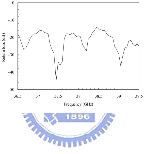
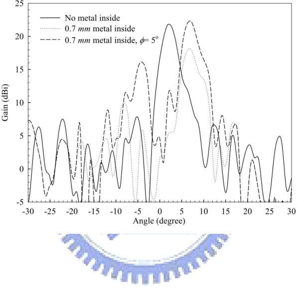
The measured gain of a single series-fed microstrip sub-array is 14.47 dBi, and the side lobe level is –9 dB. For the fabricated waveguide-fed antenna array, the measured return loss is shown in Figure 2.6. It is seen that the return loss is nearly –20 dB from 36.5 GHz to 39.5 GHz. The 10-dB bandwidth of the antenna is about 22%. The H-plane patterns with and without a metal plate inserted are shown in Figure 2.7. When there is no metal plate inside the waveguide, the gain is 21.7 dBi, the beamwidth is about 4o, the sidelobe level is –9.67dB, and the mean beam is at 1.8o. When a metal plate with the thickness of 0.7 mm is inserted on the sidewall of the waveguide, the gain is 17.95 dBi, the beamwidth is 4o, the sidelobe level is –7.07dB, and the mean beam is at 7.2o. The main beam scanning angle is 5.4o.
2.5 Conclusions
Antennas operating at millimeter wave frequencies usually suffer considerable feed line losses. Applying waveguide-fed method will result in a much less loss.
In this study, we design a waveguide-fed microstrip antenna array, and introduce a novel beam steering technique. Slightly altering the dimension of the waveguide will lead to an evident variation of propagation constant. Consequently, this is a distinctive and advanced technique of beam steering. According to the measured data, the gain of the array is near 22 dBi, the beamwidth is about 4o and the return loss is below –20 dB. The main beam scanning angle in H-plane is 5.4o, which shows good consistence with the theoretical value.
-50 -40 -30 -20 -10 0 36.5 37 37.5 38 38.5 39 39.5 Frequency (GHz) R etu rn lo ss ( dB )
Angle (degree) -30 -25 -20 -15 -10 -5 0 5 10 15 20 25 30 Ga in (dBi) -5 0 5 10 15 20 25 No metal inside 0.7 mm metal inside 0.7 mm metal inside, φ= 5o
Figure 2.7 Comparison of the H-plane patterns of the waveguide-fed microstrip antenna array at 37.8 GHz.
References
1. M-Y Li, K Chang, “New tunable phase shifters using perturbed dielectric image lines,” IEEE Trans. Micro. Theo. and Tech., vol. 46, no. 10, September 1988. 2. M-Y Li, K Chang, “Novel low-cost beam-steering techniques using microstrip
patch antenna arrays fed by dielectric image lines,” IEEE Trans. Antennas
Propagat., vol. 47, iss. 3, pp. 453-457, March 1999.
3. S. R. Rengarajan, “Slot couplers for feeding branch waveguides of a planar slot array,” IEEE AP-S Int. Symp.Digest, vol. 2, pp. 682 - 685, June 1989.
4. A. Datta, A. M. Rajeek, A Charabarty, and B. N. Das, “S matrix of a broad wall coupler between dissimilar rectangular waveguides,” IEEE Trans. Micro. Theo. and
Tech., vol. 43, no. 1, January 1995.
5. J. S. Izadian, and S. M. Izadian, Microwave transition design, Artech House, 1988. 6. T. Galia, G. Mazzarella, and G. Montisci, “A new approach to the design of linear series-fed printed arrays,” Proc. IEEE Int. Symp. Antennas Propagat, vol. 4, pp. 2736-2739, 1999.
3 A Dual-Mode Millimeter-Wave Folded
Microstrip Reflectarray Antenna
3.1 Introduction
The folded reflectarray antenna [1]-[10] presented in this chapter can be simultaneous operated in two modes, namely, the radar mode and the communication mode. In the radar mode, the antenna demonstrates high gain and narrow beamwidth characteristics with beam switching capability. It is suitable for radar applications, such as automotive sensors in wireless Intelligent Transport Systems (ITS). While in the communication mode, the beamwidth is much broader and thus provides communications over a wide angular range.
The radar is a key technology in ITS, which opens up new perspectives of comfort and safety features in future automobiles. The automotive radar can be used for target identification, road condition detection, vehicle collision warning and avoidance, obstacle warning, stop-and-go traffic support and cruise control. In addition, accurate radar images about the ambient traffic situation could be applied for multiple targets classification and scenario interpretation. For a forward looking vehicle radar, a coverage of about ±10 degree, deduced from the demand of operation in urban area or narrow road curvature, is acceptable. The required field of view can be achieved using a multi-beam or steerable beam high-resolution antenna. In general, a narrower beamwidth antenna is required to obtain higher resolution, and higher gains contribute considerably to the sensitivity.
Besides, there is an increasing trend in having a combined use of the inter-vehicle communications as well as the radar sensing. The inter-vehicle
communications play an essential role in an advanced ITS for it enables each vehicle to communicate with other vehicles (not only directly, but also indirectly via roadside communication units), so as to get the information that are difficult or impossible to measure by the vehicle alone. The vehicular collision avoidance capability can be enhanced by incorporating inter-vehicle communications technology through wireless ad hoc networks.
The design of each constituting part of the proposed antenna is presented in this chapter. Some formulas have been derived for analysis and design. Measurement results of the antenna pattern, antenna gain, aperture efficiency, and beam switching property show good agreement with the simulated ones
3.2 Principle
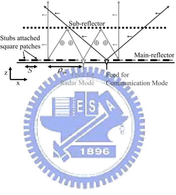
The proposed dual-mode folded reflectarray antenna is illustrated in Figure 3.1. The distance H from the main reflector to the sub-reflector is 23 mm. The main reflector is a reflectarray that consists of hundreds of square patch antennas distributed over a circular region with diameter D; each square patch has two open microstrip stubs for field twisting and phase compensation. The sub-reflector is composed of high-density printed metal lines, which is transparent to one polarization but would reflect the other. The feed antennas are probe-fed rectangular patch antennas located on the main reflector.
For the radar mode, the fields radiated from the feed antennas are polarized in the direction parallel to the metal grid lines on the sub-reflector. The fields confront the sub-reflector are reflected. Due to the path differences, the fields received by every square patch antenna on the main reflector have different phases and amplitudes. Each square patch has two open stubs to provide the required 90o polarization twisting
and phase compensation. The fields re-radiated from the square patch array are in uniform phase and tapered amplitude distribution, with polarization perpendicular to the grid lines. Thus, the re-radiated fields could penetrate through the sub-reflector and generate a narrow radiation beam.
Sub-reflector
Main-reflector
Stubs attached
square patches
Feed for
Communication Mode
Feed for
Radar Mode
S
x
z
ρ
mThe beam direction will vary with the position of the feed. Different from the single mode horn-fed multiple-beam reflectarray antennas which have already been extensively discussed [11]-[12], three feed patches were designed and implemented in the vicinity of the center of the main reflector for radar mode beam switching in this work.
On the other hand, the feed for the communication mode is designed to have a polarization perpendicular to the grid lines on the sub-reflector. Therefore, the fields radiated from this feed will transmit through the sub-reflector directly, the gain pattern is in principle that of the feed antenna, and the position of the feed antenna is not restricted to areas in the vicinity of the center of the main reflector.
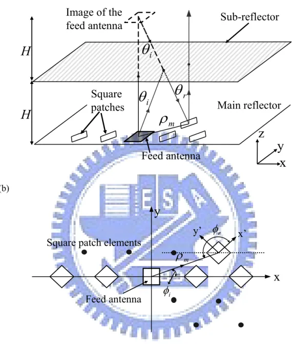
Refer to Figure 3.2. The input power fed to the feed antenna is denoted as Pi.
Gf and Gsq are the maximum gains of the feed antenna and the square patch antenna,
respectively. The antenna gains at the direction of (θ, φ) are thus correspondingly equal to Gf .gf (θ, φ) and Gsq.gsq (θ, φ), with gf (θ, φ) and gsq (θ, φ) being the
normalized power pattern of the feed antenna and the square patch antenna respectively. It is noted that, the typical pattern gf (θ, φ) of the designed feed antenna
and the measured Gf of realized antenna was used in the simulations.
The power Pm received by the mth square patch can be calculated from the
Friis’s formula and written as:
m sq f i m PG G C P = (3.1)
(a)
Image of the
feed antenna
Feed antenna
Square
patches
H
iθ
θ
r iθ
mρ
H
Main reflector
Sub-reflector
x
y
z
(b)Square patch elements
Feed antenna
rφ
mρ
x
y
x’
y’
iφ
with Cm defined as: 2 2 ) 4 ( ) 4 / 3 , ( ) , ( m i i sq i i f m r g g C π λ π φ θ φ θ ⋅ + = (3.2)
here rm (= ρm2+4H2)1/2 is the path length from the mth square patch to the feed antenna,
with ρm being the distance between the square patch and the feed antenna. For an
illuminating angle of (θi, φi) from the feed antenna, the receiving angle for the mth
square patch is (θi, φi+3π/4).
The received power by each square patch antenna will re-radiate from the same antenna. The total radiation power Prad at an angle of (θ, φ) from the in-phase
excited array is:
) , ( ) , ( ) , (θ φ G g θ φ F2 θ φ Prad = sq sq ⋅ (3.3)
where the array factor F2(θ, φ) is:
2 ) sin sin cos sin ( 2(θ,φ) jk0 xm θ φ ym θ φ m m e P F =
∑
⋅ + (3.4)with (xm, ym) being the global coordinates of the mth square patch antenna. Thus, the
total antenna gain pattern Gtotal of the folded reflectarray antenna can be derived as:
) , ( / ) , (θ φ P P G G2 f2 θ φ Gtotal = rad i = f ⋅ sq ⋅ (3.5)
where the normalized array factor is:
2 ) sin sin cos sin ( 2(θ,φ) (θ,φ) jk0 xm θ φ ym θ φ m m sq C e g f =
∑
⋅ + (3.6)3.3 Design
In this work, we developed a 38.5 GHz dual-mode folded reflectarray antenna. For radar mode beam switching operation, three fixed-position patch antennas were
created as the feeds for three corresponding spot beams. Whereas, there is another patch for the communication mode. The details for the design of each part are presented in the following subsections.
3.3.1 Feed Antenna
As a low profile folded reflectarray, feed antennas with wider beams are preferred in order to illuminate more square patch antennas. Besides, every feed’s area on the main reflector has to be small to enable multiple closely spaced beams [13]. Horn antennas are used as the feeds in general reflectarrays. A horn with sophisticated illumination design [14] would make the reflectarray have optimal aperture efficiency, but it suffers from bulky configuration and mechanical complexity. On the contrary, printed type antennas, which can be directly made on the main reflector, are advantageous to multiple-feed or movable feed design. Also, the transceiver circuits can be easily integrated on the backside of the antenna. Hence the feeds in this work are probe-fed microstrip patch antennas.
The feed patches of the folded reflectarray, having sizes (L×W) of 2.3×2.4 mm2, were designed on a Duroid 5880 substrate with thickness h of 0.508 mm and εr = 2.2.
The measured return loss of the fabricated antenna (Figure 3.11) shows a 10-dB bandwidth of 9% (from 36.5 GHz to 39.9 GHz), with a peak value of 24.8 dB. The broadside gain (Gf) is 6.3 dBi, and the measured 3-dB beamwidths in E-plane and
H-plane at 38.5 GHz are 74.7° and 88.2° respectively, as shown in Figure 3.3.
Several feed antennas, for both the radar and communication modes, will be jammed into between the dense square patch antennas on the main reflector. The close adjacency of the feed antennas and their neighboring square patch antennas will cause the depolarization effect on the feed antennas. The cross-polarization is lower than the co-polarization by at least 15 dB in simulation, which is ignorable.
However, the worst isolation is only about 5 dB by measurement. Simple treatments around periphery of the designed feed would be required to prevent the couplings, in case that the radiation pattern for communication mode is worsen, as will be discussed in Section 3.4. Whereas, in the radar mode, the narrow beam patterns after focusing will scarcely affected by the variations caused by the couplings as shown in Section 3.3.3.
-30 -25 -20 -15 -10 -5 0 5 10 -90 -60 -30 0 30 60 90 Angle (degree) Ga in ( dBi ) E plane H plane
3.3.2 Sub-reflector
Though in general, the substrate thickness of about λ/2 would allow the fields to go through the dielectric slab with minimum insertion losses [14]. The 31-mil
Duroid 5870 laminate is chosen to fabricate the sub-reflector, with fine parallel metal lines printed on, because it has a low loss tangent and its relative permittivity is close to 1. The insertion loss of a high permittivity substrate is very sensitive to the thickness. On the other hand, for low permittivity material, for example Duroid 5870, λ/2 at 38.5 GHz is around 100 mil. It is unpractical to use such a thick
laminate, despite the simulated insertion loss for this case is 0.12 dB. The simulated loss for the 31-mil Duroid 5870 substrate at 38.5 GHz is 0.51 dB, which is a quite
good value that can be obtained with commonly available laminates.
The width and spacing of the metal lines are designed so that the insertion loss is as low (high) as possible for an incident wave with its polarization perpendicular (parallel) to the metal lines. Three sub-reflectors with different printed lines were tested. The lines’ width and spacing for each sub-reflector are kept the same, and are equal to 0.1 mm, 0.2 mm, and 0.5 mm respectively. A horn antenna illuminated EM
waves toward another horn antenna at 230 mm apart. These two horns were
collimated and aligned with each other and were vertically polarized. The sub-reflectors were placed in the middle of the transmitting and receiving horns with metal lines oriented horizontally. The powers received by the receiving horn antenna were then compared to that without sub-reflector inserted. For the 0.1-mm
sub-reflector, the insertion loss due to the presence of the sub-reflector is only 0.67 dB. Then the sub-reflector was rotated to make the metal lines oriented to vertical direction, the power received with the sub-reflector is 38.49 dB lower than that without the sub-reflector. It is evident that the incident wave parallel to the metal
lines is almost totally blocked and reflected by the sub-reflector.
Note that the nonzero insertion loss represents a certain portion of the incident power will be reflected. Those waves will bounce between the main reflector and the sub-reflector, experience multi-reflection and polarization twisting, and thus would impair the antenna performance.
Although not presented here, the measurement results for the 0.2-mm and
0.5-mm sub-reflectors show that the blocking effect for the parallel incident fields
becomes worse when the line width and spacing increases. Thus, the 0.1-mm
sub-reflector was adopted for use in the folded reflectarray.
3.3.3 Main Reflector
The efficiency of a reflectarray is usually not that high as compared to a conventional reflector antenna. The reduction in efficiency results from the power losses in the stubs-attached patch elements and the phase and polarization errors due to mutual coupling between non-identical elements. Besides, in a folded type antenna, there are extra losses in the path because the reflected fields by the sub-reflector are no greater than the incident fields, and thus the efficiency would be lower. Although the typical values for reflectarrays range from 10% to 30%, efficiency up to 70 % has been reported [15]. The aperture efficiency (η) is defined as: 2 max 2 max ) / ( ) / 4 ( π λ π λ η D G A G p = ⋅ = (3.7)
here Ap (= πD2/4) is the area of the main reflector and Gmax is the maximum antenna
gain.
arranged to form an equilateral triangular array with spacing S equal to 5 mm, or about 0.6λ, within a circular area with diameter D. In general, the aperture efficiency for a small reflectarray, even with reasonable good illumination, is not very good, but gets much better with increasing size and adapted illumination.
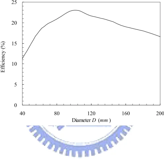
Figure 3.4 shows the calculated aperture efficiency of the folded reflectarray antenna as a function of D when illuminated by the same feed patch. As the antenna size increases, the efficiency first increases due to the fast growth of the antenna gain. Then, when D is further increased, the efficiency slightly decreases. This is because that the illumination power decreased as the distance and angle from the feed patch increases; the received power of the square patch antenna decays rapidly as the patch moves far away from the feed antenna, and thus the gain of the whole reflectarray becomes saturated. A maximum calculated efficiency of about 25% could be achieved as D equals 140 mm. However, when D becomes larger than 100 mm, the efficiency growth by enlarging the array size is quite limited, since the normalized received powers of the square patches located outside the circular region of radius 50
mm are below –8.3 dB. Therefore, D is determined to be 100 mm in this work.
The same substrate material as that for the feed antenna was used to fabricate the main reflector. The main reflector comprises several hundreds of square patch antennas located inside a circular area of diameter D = 100 mm. The square patch antennas are oblique to the feed antenna with 45°. For field twisting and focusing, two microstrip open stubs, each with a λ/4 impedance transformer, are attached to two adjacent edges of the square patch, as shown in Figure 3.5. The square patch measures 2.3×2.3 mm2. The widths of the stubs and the transformers are, respectively, 0.17 mm and 0.1 mm. The field incident on the antenna will be received by the two stubs, reflected at the open end, and then fed back to the antenna
for re-radiation. The difference between the open stubs’ lengths is designed to be
λ/4. This will make the re-radiated field orthogonal to the incident field, as will be explained in the next paragraph. Besides, the absolute lengths of the stubs are determined according to the location of each square patch so as to compensate the phase delay due to path differences. Therefore, the antennas on the main reflector are excited with uniform phase and tapered amplitude distribution.
0 5 10 15 20 25 40 80 120 160 200 Diameter D (mm ) E ff ici en cy ( % ) .
Figure 3.4 Calculated aperture efficiency, as a function of the aperture’s diameter D of the folded reflectarray antenna.
To see the field twisting effect, let us consider a vertical field (radiated from the feed antenna) incident on the stubs-attached patch. As shown in Figure 3.5(a), the incident field can be decomposed into two orthogonal components, that is, component A and component B. These two equal-amplitude components are separately received by the two orthogonal open stubs on the left and right sides. After reflected at the stubs’ open ends, these components are fed back to the antenna. Since the left stub is longer than the right stub by λ/4, component A experiences 180° more phase delay than component B in the round-trip tour. The resultant total re-radiation field is thus twisted to the horizontal direction, as shown Figure 3.5(b).
For better estimation of the folded reflectarray’s performance, scattering parameters of the individual square patch antenna was measured by extending the two open stubs as two ports. Around the design frequency of 38.5 GHz, the return loss (S11) and isolation between ports (S21) are less than –20 dB. Also, the
co-polarization and cross-polarization patterns were taken with one port terminated. The broadside gain and the 3-dB beamwidth of the co-polarization component are 5.6 dBi and 88° respectively. By putting the measured patterns of the individual square patch into (5), a co-polarization gain of about 26 dBi and a maximum cross-polarization gain (assumed the cross-polarization fields of the square patches were in-phase) of –4.8 dBi of the folded reflectarray were obtained.
(a) (b)
Figure 3.5 The field twisting effect of the 45° tilted square patch antenna with two open stubs.
Furthermore, derived from the full wave simulation result of the single square patch with appropriate periodic boundary conditions applied, the maximum cross-polarization of the folded reflectarray grows up from –4.8 dBi to about –1.5 dBi. It is the mutual coupling effect by the close proximity of the square patches and the stubs. Actually, the cross-polarization component of the array is at least 27.5 (=26–(–1.5)) dB lower than the co-polarization component of the array, which is very small and will be blocked by the sub-reflector.
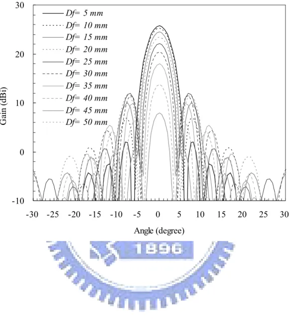
For more efficient use of the excitation power and suppressing the pattern ripple, the feed antennas for radar mode should be placed as near the center of the array as possible. Square patch antennas overlap the feed antennas are to be detached for the accommodation of the feed antennas. Therefore, since the effective aperture reduces, the main beam gains will decrease and the side lobes will increase. Assume that there are no square patch antennas within the circular area of diameter Df. The
simulated patterns for various Df are shown in
Figure 3.6. When Df = 30 mm, the gain drops about 1.27 dB in comparison to
Df = 0 mm. In reality, the feeds will occupy an area substantially less than that of the
Df = 30 mm circle. The pattern will not be significantly affected.
It is also known from the simulations that the scattered fields reflected by the ground plane of the main reflector are relatively weak, in comparison to the fields re-radiated from the square patches. Moreover, the ground scatterings are haphazardly distributed; they do not lead to co-phasal behavior in any direction and thus were ignored in the design.
-10 0 10 20 30 -30 -25 -20 -15 -10 -5 0 5 10 15 20 25 30 Angle (degree) Ga in ( dBi ) . Df= 5 mm Df= 10 mm Df= 15 mm Df= 20 mm Df= 25 mm Df= 30 mm Df= 35 mm Df= 40 mm Df= 45 mm Df= 50 mm
Figure 3.6 Calculated H-plane patterns of the folded reflectarray antenna for various
3.3.4 Beam Switching Mechanism
As can be seen from Figure 3.2 that, by moving the position of the feed antenna, the path length from the image feed antenna to the mth square patch changes from the original value rm to a new value rm’, and then the new normalized array factor
becomes: 2 ) sin sin cos sin ( 2( , ) ( , ) jk0 xm ym rm m m sq C e g f θ φ = θ φ
∑
⋅ θ φ+ θ φ+Δ (3.8)the path length variation for a small feed movement has negligible influence on the received power (Pm), but the shift k0Δrm (=k0(rm-rm’)) in the phase term of the antenna
gain pattern would result in a beam direction change.
Figure 3.7 shows the calculated H-plane gain patterns for various displacements
d of the feed position. The feed antenna moves along the x direction from d = –15 mm to +15 mm. When d = 0 mm, the radiation beam points to the broadside
direction, with the antenna gain of 25.73 dBi, 3-dB beamwidth of 4.9°, and side lobe levels of about –25 dB. It is seen that, as d changes from –15 mm to +15 mm, the main beam directs from +14.4° to –14.4°, the corresponding first side lobe moves from the left hand side of the main beam to the right hand side, and the side lobe level rises with the increase of the feed position displacement. The beam steering rate is about 1° per 1 mm movement. However, the antenna gain becomes lower as the feed moves farther away from the center position. The maximum gain variation in the range of d = –15 mm to +15 mm is about 1.5 dB.
A sliding track mechanism, as shown in Figure 3.8, which allows controlling the movement of the feed, was fabricated to verify the above analysis. The center region of the main reflector was dug out so that the feed antenna can be placed and moved. The total movable range is 8 mm (d = –4 mm to +4 mm). The measured H-plane
patterns of the folded reflectarray antenna for various feed positions (d) at 38.5 GHz are illustrated in Figure 3.9. A total steering angle of 7.2° was attained for the 8-mm feed position displacement. The beam steering rate is very close to the simulated one.
-10 -5 0 5 10 15 20 25 30 -30 -25 -20 -15 -10 -5 0 5 10 15 20 25 30 Angle (degree) G ai n (d B i) . d= -15mm d= -12.5mm d= -10mm d= -7.5mm d= -5mm d= -2.5mm d= 0mm d= 2.5mm d= 5mm d= 7.5mm d= 10mm d= 12.5mm d= 15mm d
Figure 3.7 Calculated H-plane patterns of the folded reflectarray antenna for various displacements (d) of the feed position at 38.5 GHz.
Figure 3.8 Bottom view (left) and top view (right) of the sliding track mechanism, which is mounted with the main reflector.
3.4 Results
Figure 3.10 shows the photo of the finished folded reflectarray antenna with the sub-reflector uncovered. An aluminum ring wall with inner diameter of 128 mm and height of 23 mm was used as the housing to support and separate the two reflectors. The three feeds for the radar mode are lined up along the x direction, with the intervals being 12.5 mm, and located at the center of the main reflector. While the feed for the communication mode is not on the same line as the radar mode feeds and away from the center by about 14.2 mm. The measurement results for both modes are presented in the following subsections.
3.4.1 Radar Mode
The measured return loss of the finished folded reflectarray for d = 0 mm feed is shown in Figure 3.11. It is –22.4 dB at 38.5 GHz. Figure 3.12 illustrates the measured H-plane patterns of the folded reflectarray antenna for various feed positions (d) at 38.5 GHz. Simulation results are also shown for comparison. It is seen that, as d changes from –12.5 mm to +12.5 mm, the main beam directs from +14.9° to –14.6°. The beam steering rate is a little larger than 1° per 1 mm movement, while the simulated main beam directions are +11.875o and –11.875o for
d = –12.5 mm and d = +12.5 mm respectively. The measured gains of the antenna
for d = –12.5 mm, d = 0 mm, and d = +12.5 mm are 22.5 dBi, 27.4 dBi and 22.6 dBi respectively. The maximum aperture efficiency is about 33.9%, which is better than the simulated one of 23.0%. The measured 3-dB beamwidths are 4.9o in the E-plane and 4.4° in the H-plane. Besides, the measured side lobe levels are –15.5 dB in the E-plane and –18.8 dB in the H-plane.
Figure 3.9 The measured H-plane patterns for various feed positions (d) at 38.5 GHz.
-30 -25 -20 -15 -10 -5 0 36 37 37 38 38 39 39 40 40 Frequency (GHz) S1 1 ( dB ) .
Folded Reflectarray Antenna Feed Patch
Figure 3.11 The measured return losses of the fabricated folded reflectarray antenna for d= 0 mm feed in the radar mode, and the single feed patch.
-10 -5 0 5 10 15 20 25 30 -90 -60 -30 0 30 60 90 Angle (degree) Ga in ( dB i) . d= -12.5mm (measured) d= 0mm (measured) d= 12.5mm (measured) d= -12.5mm (simulated) d= 0mm (simulated) d= 12.5mm (simulated) d
Figure 3.12 The radar mode H-plane patterns of the folded reflectarray antenna at 38.5 GHz for various feed positions (d).
The measurement results agree well with the simulations in the main beam region, yet behave worse in the side lobe areas owing to the blockage of the feed antennas and the phase errors caused by mutual couplings between the square patches. Also, parts of the waves reflected at the grid lines are re-reflected at the main reflector and spreading around in the antenna, leading to increased side lobes.
In fact, the beam scanning angle introduced by placing the feed off the focal point decreases with focal length to diameter ratio for a reflector antenna. Nonlinear phase as a function of feed displacement leads to pattern distortion, including beam broadening, rise in side lobe levels, and gain loss. These effects worsen with increasing feed displacement for a reflector antenna with a short focal length like this [16].
3.4.2 Communication Mode
The communication mode is expected to have a pattern resembles that of the feed patch. Unfortunately, the measured pattern exhibits a high ripple level. The major reason would be that, on the main reflector, the square patch elements in the close proximity of the communication mode feed patch would be excited by the couplings from that feed, and the radiations from those excited square patch elements would spoil the pattern. In addition, the cross-polarization component of the communication mode feed operates in the radar mode, which will be reflected by the sub-reflector and then re-radiated from the square patches, so that the pattern will be interfered. The introduction of the sub-reflector would be another influential factor.
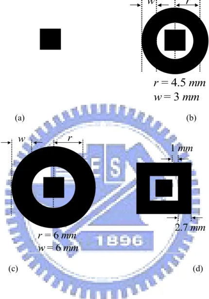
In order to ameliorate the ripple level, the sub-reflector was first removed, and then the effects of various treatments on the feed patch for the communication mode were investigated. The feed patch was enclosed by metal traces with different shapes and widths. Some of the most efficient methods are illustrated in Figure 3.13.
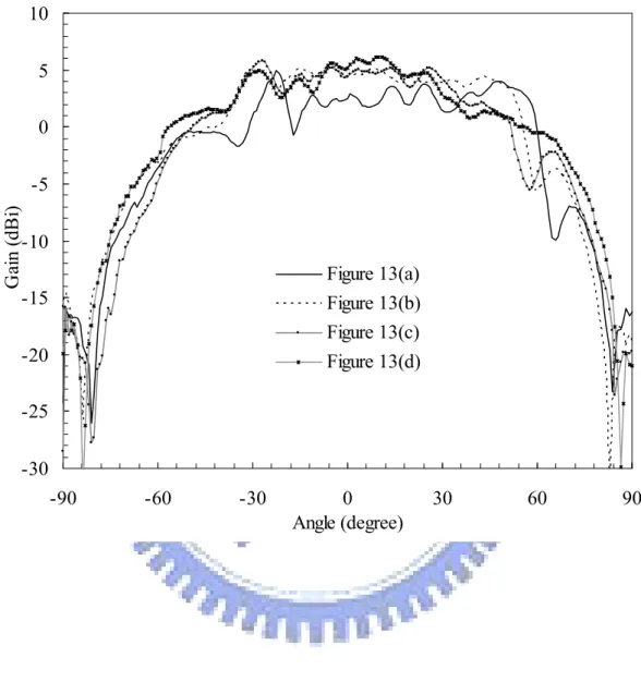
It is obvious that, with the metal traces, the patterns have been considerably improved, as shown in Figure 3.14. The case that the feed patch surrounded by a metal square frame (Figure 3.13(d)) was selected and implemented, because its pattern is most similar to that of a typical patch antenna and has the most mitigated fluctuations. The co-polarization pattern becomes smoother and more symmetric, and the gain is slightly increased. This decision is also corroborated by the fact that the measured cross-polarization fields are at least 10 dB lower than that without the metal square frame, as shown in Figure 3.15. The measured return losses of the finished folded reflectarray for various feed antennas presented in Figure 3.13 at 38.5 GHz are shown in Figure 3.16. The return loss at 38.5 GHz for the case with Figure 3.13(d) as the feed is –21.4 dB.
Then, the sub-reflector was re-installed while keeping the square frame enclosed patch (Figure 3.13(d)) as the feed. The measured pattern is shown in Figure 3.17. The pattern of using the original patch as the feed (Figure 3.13(a)), with the sub-reflector installed, is also shown for comparison. It can be seen that the modification made to the feed has alleviated the sharp dips, and raised the averaged gain by about 2dB, especially near the broadside direction (e.g. –30o to +30o). Although the ripples are not thoroughly removed, this pattern performs satisfactorily for the inter-vehicle communications, which is an application of short-range wireless technology.
r = 4.5 mm
w = 3 mm
r
w
(a) (b)r = 6 mm
w = 6 mm
1 mm
2.7 mm
r
w
(c) (d)Figure 3.13 Four communication mode feed antennas: (a) The original feed patch described in section 3.3. (b) The original feed patch enclosed with a metal ring trace. The width of the trace (w) is 3 mm and the radius of the ring (r) is 4.5 mm. (c) The original feed patch enclosed with a larger metal ring trace. Both the width of the trace (w) and the radius of the ring (r) are 6 mm. (d) The original feed patch enclosed by a metal square frame, with the trace width being 2.7 mm and the gap being 1 mm.
-30 -25 -20 -15 -10 -5 0 5 10 -90 -60 -30 0 30 60 90 Angle (degree) Ga in ( dB i) . Figure 13(a) Figure 13(b) Figure 13(c) Figure 13(d)
Figure 3.14 The measured patterns for various feed antennas presented in Figure 3.13, with the sub-reflector removed.
Angle (degree) -90 -60 -30 0 30 60 90 Cr oss-p ol arizati on (dB i) -40 -35 -30 -25 -20 -15 -10 -5 0 Fig. 13(a) Fig. 13(b) Fig. 13(c) Fig. 13(d) Figure 13(a) Figure 13(b) Figure 13(c) Figure 13(d)
Figure 3.15 The measured cross-polarization patterns for various feed antennas presented in Figure 3.13, with the sub-reflector removed.
-30 -25 -20 -15 -10 -5 0 36 37 37 38 38 39 39 40 40 Frequency (GHz) S1 1 ( dB ) Figure 13(a) Figure 13(b) Figure 13(c) Figure 13(d)
Figure 3.16 The measured communication mode input reflection coefficients of the fabricated folded reflectarray antenna, for various feed antennas presented in Figure 3.13.
-30 -25 -20 -15 -10 -5 0 5 10 -90 -60 -30 0 30 60 90 Angle (degree) G ain (d B i) . Figure 13(a) Figure 13(d)
Figure 3.17 The measured patterns at 38.5 GHz, with sub-reflector, for: (a) original feed patch (Figure 3.13(a)), (b) original feed patch enclosed by a metal square frame (Figure 3.13(d)).