F
H
U
R
EALIZED
V
OLATILITY
YU-SHENG LAI* HER-JIUN SHEU
A number of prior studies have developed a variety of multivariate volatility mod-els to describe the joint distribution of spot and futures, and have applied the results to form the optimal futures hedge. In this study, the authors propose a new class of multivariate volatility models encompassing realized volatility (RV) estimates to estimate the risk-minimizing hedge ratio, and compare the hedging performance of the proposed models with those generated by return-based mod-els. In an out-of-sample context with a daily rebalancing approach, based on an extensive set of statistical and economic performance measures, the empirical results show that improvement can be substantial when switching from daily to intraday. This essentially comes from the advantage that the intraday-based RV potentially can provide more accurate daily covariance matrix estimates than RV uti-lizing daily prices. Finally, this study also analyzes the effect of hedge horizon on hedge ratio and hedging effectiveness for both the in-sample and the out-of-sample data. © 2009 Wiley Periodicals, Inc. Jrl Fut Mark 30:874–896, 2010
The authors thank Robert Webb (the Editor) and an anonymous referee for their very constructive sugges-tions, the National Science Council in Taiwan for financial supports (NSC 96-2416-H-260-022-MY3). *Correspondence author, Department of Management Science, National Chiao Tung University, 1001 Da Hsueh Road, Hsinchu 30050, Taiwan. Tel: ⫹886-3-5712121 ext. 57101, Fax: ⫹886-3-5713796, e-mail: [email protected]
Received August 2008; Accepted September 2009
■ Yu-Sheng Lai is a Ph.D. candidate in the Department of Management Science, National Chiao Tung University, Hsinchu, Taiwan.
■ Her-Jiun Sheu is a Professor in the Department of Banking and Finance, National Chi Nan University, Nantou, Taiwan.
The Journal of Futures Markets, Vol. 30, No. 9, 874–896 (2010) © 2009 Wiley Periodicals, Inc.
INTRODUCTION
A considerable amount of studies on futures hedging have focused on modeling the joint distribution of spot and futures prices and applying the results to esti-mate the optimal hedge ratio. Although the early studies assume that the hedge ratio is constant over time (e.g., Ederington, 1979), recent studies have docu-mented that the joint distribution, and hence the hedge ratio, should be time dependent due to the time-varying nature of risks (e.g., Kroner & Sultan, 1993).1 Since then, varieties of multivariate volatility techniques have been applied. Baillie and Myers (1991), Myers (1991), Kroner and Sultan (1993), Brooks, Henry, and Persand (2002), Lien, Tse, and Tsui (2002), and Lien and Yang (2006) are examples of studies that apply generalized autoregressive condi-tional heteroscedasticity (GARCH) models.2As a result, the central issue in the context of a dynamic hedge is to provide the conditional covariance matrix fore-cast that can characterize the dynamics of the distribution more realistically.
However, it has been shown that most of the latent GARCH models fail to satisfactorily describe the high kurtosis, small first-order autocorrelation of squared returns, and slow decay of the autocorrelation of squared returns toward zero that have been observed in many daily or weekly financial returns (e.g., Carnero, Peña, & Ruiz, 2004).3The search for alternative volatility tech-niques has motivated scholars to exploit information in intraday high-frequency data (e.g., Andersen & Bollerslev, 1998; Andersen, Bollerslev, Diebold, & Labys, 2003; Barndorff-Nielsen & Shephard, 2004; Hayashi & Yoshida, 2005; Voev & Lunde, 2007). This so-called realized volatility (RV) approach provides a direct and consistent technique to estimate the latent volatility process with-out the need for relying on explicit models.4 Therefore, it has served as an ex-post benchmark for assessing the quality of any ex-ante volatility forecasts (e.g., Andersen, Bollerslev, Christoffersen, & Diebold, 2006). In forecasting future volatility, studies have shown that RV can provide more accurate forecasts than methods using daily squared returns (e.g., Blair, Poon, & Taylor, 2001). Recently, RV has been employed to explore the economic value (EV) of invest-ment by Fleming, Kirby, and Ostdiek (2003), Bandi, Russell, and Zhu (2008),
1With the aim of reducing risk, this hedge ratio is equivalent to the ratio of the conditional covariance
between the spot and futures over the conditional variance of the futures.
2In addition to the GARCH framework, other studies use stochastic volatility models (e.g., Lien & Wilson,
2001).
3To capture the high kurtosis of returns and low first-order autocorrelation of return squares simultaneously,
GARCH models often require a high persistence and/or leptokurtic conditional distributions when they are fitted to the financial time series (Carnero et al., 2004). The restrictions on GARCH then severely restrict the allowed dynamic dependence of the volatility.
4Generally, in the absence of market microstructure and nonsynchronous trading (Epps effect), a daily
meas-ure of variance is computed as the sum of the squared intraday equidistant returns, and a daily measmeas-ure of covariance is obtained by summing the products of intraday equidistant returns, for the given trading day. For a review of the RV refers to McAleer and Medeiros (2008).
and De Pooter, Martens, and van Dijk (2008).5 They find that the EV is sub-stantial when switching from daily to intraday returns, even without applying bias-correction techniques in constructing realized estimates. As a result, the superiority of RV-based investment may result because it takes into account finer intraday information and thus potentially provides more accurate daily covariance matrix estimates or forecasts than methods utilizing daily prices.
This study attempts to improve the performance of a risk-minimizing futures hedge when the intraday-based RV approach is incorporated into fore-casting the relevant covariance matrix. It is not clear, however, whether the accurate RV is used or not may differentiate the performance of a futures hedge. To address this issue, a new RV-based method is demonstrated in this study. The proposed method builds on the bivariate error correction model by employing the flexible constant conditional correlation (CCC) GARCH error structure of Kroner and Sultan (1993). The advantage of extending their model is that it can capture the long-run cointegration relationship and the time-varying second moments simultaneously when the dynamics of the joint distribution is specified. Moreover, when the leverage effect and/or the dynamic correlation are revealed, the asymmetric volatility and/or the dynamic conditional correla-tion (DCC) models can also be incorporated into this method. These desirable properties thus provide a more convenient way to lodge the realized covariance matrix in the GARCH error structures as compared with the rolling estimators of Fleming et al. (2003), Bandi et al. (2008), and De Pooter et al. (2008). The RV-based method, which uses finer volatility proxies in estimating and forecast-ing the conditional covariance matrix, is expected to provide better descriptions on the spot-futures dynamics and the resulting hedge ratios than methods using squared return shocks.
In the empirical analyses, the RV-based hedge ratios are calculated in an out-of-sample context spanning the period of December 19, 2003 through March 31, 2009 for the highly traded S&P 500 index futures contracts. We compare the performance of the RV-based hedge with the return-based GARCH and the ordinary least squares (OLS) hedges using an extensive set of statistical and economic measures. The comparisons are conducted for both short and long hedgers. To anticipate the results, this study finds that the RV-based hedge can substantially outperform the return-RV-based GARCH and/or the static OLS hedges especially during the surge in volatility period. Then the RV-based method is applied to examine the effect of hedging horizon (ranges from
5For example, Fleming et al. (2003) show how a risk-averse investor would be willing to pay 50–200 basis
points per year to capture the multivariate volatility forecasts based on intraday returns instead of daily returns in the context of investment decisions on three actively traded futures contracts (S&P 500 index, Treasury bonds, and gold). It is assumed that the investor follows a volatility-timing strategy, which rebal-ances his portfolio only when the estimated conditional covariance matrix of the daily returns changes. This case treats the expected daily returns as time-invariant.
one week to three month) on hedge ratio and hedging effectiveness. The results show that hedge ratio tends to increase and to approach unity (i.e., naïve hedge ratio) with the length of hedging horizon; and, hedging effectiveness tends to increase as the length of hedging horizon increases. The rest of the study is organized as follows. First, we present the conventional hedging method and demonstrate the RV-based method used in this study. Next, we present the data and their properties with the empirical results. Finally, the last section con-cludes the study.
THE CONVENTIONAL HEDGING MODELS
Kroner and Sultan (1993) have proposed a bivariate GARCH error correction model for modeling the joint distribution of spot and futures. As such, the most prominent application of this model is to estimate time-varying hedge ratios. Let rs,tand rf,tdenote, respectively, the changes in the logarithmic spot price, St, and the logarithmic futures price, Ft, between time t⫺ 1 and t. The economet-ric model for the daily returns conditioning on the set of all relevant informa-tion⌽t⫺1at time t⫺ 1 can be described as
(1)
(2) where (St⫺1⫺ dFt⫺1) is the error correction term (ECT). The incorporation of ECT in the conditional mean equations is essential, especially in currency and equity markets (see Brooks et al., 2002; Choudhry, 2003; Park & Switzer, 1995). The residual vector (es,t, ef,t)⬘ is postulated as a bivariate normal distribution with a 2 ⫻ 1 zero mean vector and a 2 ⫻ 2 time-varying covariance matrix
(3) where hsf,tis a conditional covariance, and hs,tand hf,tare conditional variances for the spot and futures returns, respectively, and r is the time-invariant corre-lation coefficient between them. That is, the model applies the CCC estimator of Bollerslev (1990) to model and forecast the bivariate conditional covariance matrix.
The expressions of the conditional variances hs,t and hf,tin Equation (3) are typically thought of as univariate GARCH-type models. For example, the
Ht⫽ c hs,t hsf,t hsf,t hf,t d ⫽ ch1兾2s,t 0 0 h1兾2f,t d c1 r r 1d c h1兾2s,t 0 0 h1兾2f,t d ⫽ DtRDt aes,t ef,tb ` £t⫺1⬃ N(0, Ht) rf,t⫽ a0f⫹ a1f(St⫺1⫺ dFt⫺1) ⫹ ef,t rs,t⫽ a0s⫹ a1s(St⫺1⫺ dFt⫺1) ⫹ es,t
GARCH(1,1) structure introduced by Bollerslev (1986) for the returns can be specified as
(4) When the leverage effect is revealed, asymmetric volatility models are commonly formulized, such as the GJR (Glosten–Jagannathan–Runkle) model of Glosten, Jagannathan, and Runkle (1993). This simply modifies the stan-dard GARCH(1,1) model with an additional ARCH (autoregressive conditional heteroscedasticity) term conditional on the sign of the past innovation. The conditional volatilities of Equation (4) are then reformulated as
(5) where I(⭈) denotes an indicator function. For estimating the constant correla-tion coefficient, the ever-popular rolling estimator uses equal weight to all past
T return innovations:
(6)
To fit in with reality, however, the conditional correlation coefficient can be relaxed to vary with time (Engle, 2002; Tse & Tsui, 2002). That is, the condi-tional covariance matrix of Equation (3) is generalized to the DCC formulation: (7) The evolution of rt in this study is analogous with the univariate GARCH equation:
(8)
where u1and u2 are nonnegative with u1⫹ u ⱕ 1; the sample size M ⫽ 2 for
estimating the sample correlation coefficient with (i⫽ s, f )
follows Tse and Tsui (2002); is the unconditional correlation between spot and futures.
r
hi,t⫺h⫽ ei,t⫺h兾h1兾2i,t⫺h
rt⫽ (1 ⫺ u1⫺ u2)r⫹ u1rt⫺1⫹ u2 aMh⫽1hs,t⫺hhf,t⫺h Ba a M h⫽1h 2 s,t⫺hba a M h⫽1h 2 f,t⫺hb Ht⫽ c hs,t hsf,t hsf,t hf,t d ⫽ ch1兾2s,t 0 0 h1兾2f,t d c1 rt rt 1d c h1兾2s,t 0 0 h1兾2f,t d ⫽ DtRtDt rˆ ⫽ aTt⫽1es,tef,t Ba a T t⫽1e 2 s,tba a T t⫽1e 2 f,tb 僆 [⫺1,1] hf,t⫽ b0f ⫹ b1fhf,t⫺1⫹ b2fe2f,t⫺1⫹ b3fe2f,t⫺1I(ef,t⫺1 ⬍ 0) hs,t⫽ b0s⫹ b1shs,t⫺1⫹ b2se2s,t⫺1⫹ b3se2s,t⫺1I(es,t⫺1 ⬍ 0) hf,t⫽ b0f⫹ b1fhf,t⫺1⫹ b2fe2f,t⫺1 hs,t⫽ b0s⫹ b1shs,t⫺1⫹ b2se2s,t⫺1
Given the null hypothesis that the set of all relevant information ⌽t⫺1 is observed with correctly specified models, these CCC or DCC models with the ECT describe the dynamic nature of spot-futures distributions. In particular, this GARCH class of volatility (correlation) models provides simple ways to forecast the bivariate volatility by using actual return innovations and the esti-mated hedge ratio by minimizing the risk of the hedged portfolio return at time
t is given by
(9) where and are the covariance and variance forecasts using Equations (3) or (7). In brief, Equations (1) through (9) then construct the conventional hedge ratio models, namely, the ECT-GARCH-CCC model (Equations (1)–(4), (6), and (9)), the ECT-GARCH-DCC model (Equations (1)–(2), (4), and (7)–(9)), the ECT-GJR-CCC model (Equations (1)–(3), (5)–(6), and (9)), and the ECT-GJR-DCC model (Equations (1)–(2), (5), and (7)–(9)).
ALTERNATIVE MODELS USING RV
To explore the incremental value of a RV-based hedge, the realized variance and/or correlation are encompassed within the conventional CCC and DCC models with the ECT specification. Following the previous specifications, the RV-based GARCH(1,1) volatility can be expressed as
(10) where each RVi,t⫺1 (i ⫽ s, f ) is defined by summing up ⌬-minute squared returns at time t⫺ 1. Analogously, the RV-based GJR(1,1) model can be refor-mulated as
(11) That is, the right-hand side squared residuals in the conventional GARCH or GJR models are replaced by realized variances. To encompass the realized correlation RCorrt⫺1⫽ RCovt⫺1/(RVs,t⫺1RVf,t⫺1)1/2within the conditional corre-lation dynamics, Equation (8) can be modified as
(12) where the realized covariance RCovt⫺1 is defined by cumulating the cross-products of intraday spot and futures returns at time t⫺ 1. For estimating the
rt⫽ (1 ⫺ u1⫺ u2)r⫹ u1rt⫺1⫹ u2RCorrt⫺1 hf,t⫽ b0f⫹ b1fhf,t⫺1⫹ b2fRVf,t⫺1⫹ b3fRVf,t⫺1I(ef,t⫺1 ⬍ 0) hs,t⫽ b0s⫹ b1shs,t⫺1⫹ b2sRVs,t⫺1⫹ b3sRVs,t⫺1I(es,t⫺1 ⬍ 0) hf,t⫽ b0f⫹ b1fhf,t⫺1⫹ b2fRVf,t⫺1 hs,t⫽ b0s⫹ b1shs,t⫺1⫹ b2sRVs,t⫺1 hˆf,t⫹1 hˆsf,t⫹1 bˆ*t⫽ hˆsf,t⫹1兾hˆf,t⫹1
constant correlation in the RV-based CCC model, however, the sample mean of the realized correlations should be a biased estimate due to nonsynchronous trading (Epps effect) and/or market microstructure noise (see, e.g., Hayashi & Yoshida, 2005; Voev & Lunde, 2007). To simplify the estimation process, the rolling estimator of Equation (6) is still adopted. Then, these modifications con-struct a new class of RV-based hedge ratio models, namely, the ECT-RV-GARCH-CCC model (Equations (1)–(3), (6), (9), and (10)), the ECT-RV-GARCH-DCC model (Equations (1)–(2), (7), (9), (10), and (12)), the ECT-RV-GJR-CCC model (Equations (1)–(3), (6), (9), and (11)), and the ECT-RV-GJR-DCC model (Equations (1)–(2), (7), (9), and (11)–(12)).
To estimate the parameters in the RV-based or the conventional CCC or DCC models, we follow the two-step estimation procedure of Bollerslev (1990) and Engle (2002). As this class of multivariate volatility models has separate parameters, it can be estimated easily and consistently in two steps.6With the normality assumption of Equation (2), we can maximize each volatility term with the conditional mean in the first step:
(13) where qi⫽ (ai, bi, d) and denote the Gaussian quasi-likelihood function for asset i, and then maximize the correlation term:
(14) in the second step, LCrepresents the Gaussian quasi-likelihood function of the correlation part, and u⫽ r for the CCC and u ⫽ (u1, u2) for the DCC. Without the normality assumption, these estimators still have the quasi-maximum like-lihood interpretation.
EMPIRICAL ANALYSES Data Descriptions
The performance of the RV-based hedging method is examined empirically on the S&P 500 index futures contracts traded on Chicago Mercantile Exchange (CME). The sample period is from January 1, 1998 to March 31, 2009, which covers the period of subprime mortgage crisis. We obtain the daily closing (set-tlement) prices for the spot (futures) from the Datastream and the intraday
uˆ⫽ arg max 5LC(u0ˆ)6
LVi
ˆi⫽ arg max 5LVi(i)6
6Engle and Granger (1987) indicate that a cointegration system could consistently be estimated via a two-step estimator, where both two-steps require only single equation least squares, so that we can estimate the DCC-type models with the ECT by using the two-step procedure of Bollerslev (1990) and Engle (2002).
transaction prices for them from Tick Data Inc.7Note that this study rolls the nearest month contract to the next month when the daily volume of the current contract is exceeded. Specifically, daily and intraday prices of all days corre-sponding to U.S. public holidays are removed. Hence, there are 2828 trading days for the period examined.
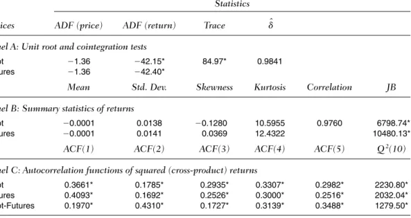
Table I reports the diagnostic checks on the distribution properties of the daily spot (futures) returns, which are calculated as differenced natural loga-rithmic daily closing (settlement) prices. The results of unit root and cointegra-tion tests are shown in Panel A, and summary statistics on the returns are reported in Panel B. The augmented Dickey–Fuller tests show that the spot and futures log-prices have a unit root, but their first-differenced series are sta-tionary. The Johansen trace statistic indicates that the spot and futures prices are cointegrated with the cointegrating parameter . The unconditional distributions of the univariate returns reveal nonnormality, as evidenced by the nonzero skewness, high kurtosis, and significant Jarque–Bera statistics. Panel C
dˆ ⬇ 1
TABLE I
Data Description: Daily Price Returns Statistics Indices ADF (price) ADF (return) Trace ˆd Panel A: Unit root and cointegration tests
Spot ⫺1.36 ⫺42.15* 84.97* 0.9841
Futures ⫺1.36 ⫺42.40*
Mean Std. Dev. Skewness Kurtosis Correlation JB Panel B: Summary statistics of returns
Spot ⫺0.0001 0.0138 ⫺0.1280 10.5955 0.9760 6798.74*
Futures ⫺0.0001 0.0141 0.0369 12.4322 10480.13*
ACF(1) ACF(2) ACF(3) ACF(4) ACF(5) Q2(10)
Panel C: Autocorrelation functions of squared (cross-product) returns
Spot 0.3661* 0.1785* 0.2935* 0.3307* 0.2982* 2230.80*
Futures 0.4093* 0.1692* 0.2526* 0.3000* 0.2516* 2032.04*
Spot-Futures 0.1970* 0.4310* 0.1727* 0.3139* 0.3488* 1279.50*
Notes. The daily spot (futures) returns are calculated as differenced natural logarithmic closing (settlement) prices where public
hol-idays are removed. The sample period for the prices runs from January 1, 1998 to March 31, 2009 and the sample size for each is 2,828. The values in rows ADF, Trace, JB, ACF(k ), and Q2(10) are statistics of the augmented Dickey–Fuller unit root test, the Johansen cointegration test, the Jarque–Bera normality test, the order k autocorrelation of squared returns, and the Ljung–Box test for the serial correlations in the squared returns. ˆd is the estimated cointegrating parameter. * indicate significance at the 5% level.
7The intraday transaction observations consist of open, high, low, and close prices at the one-minute
provides the autocorrelation functions (ACF) as well as the Ljung–Box statis-tics of the squared (cross-product) daily returns. The first-order ACF ranges from 0.1970 to 0.4093 but decays slowly toward zero. Based on the empirical evidences and the findings of Carnero et al. (2004), the conventional GARCH models may be inadequate to describe the spot-futures volatility dynamics, hence, it is not clear whether the inadequacy may damage the performance of a futures hedge.
To construct the realized (co-)variance for the alternative method, the intra-day futures prices after 3:00 p.m. Chicago time for each intra-day t are dropped as the futures market closes 15-minutes later than the spot market.8We divide the contemporaneous time section across the markets, which runs from 8:30 a.m. until 3:00 p.m. (390-minutes), into m (nonoverlapping) intervals of equal lengths ⌬ ⫽ 390/m such that the times tj⫽ tj⫺1⫹ ⌬ for j ⫽ 1, . . . , m with t0⫽ 8:30 a.m. Chicago time. The log close price at time tjis denoted as p(tj), then the equidis-tant intraday returns on day t, , for j⫽ 2, . . . , m; and, the first
period (j⫽ 1) intraday returns are defined as the difference between the log close and open prices during that time interval. With these mathematical defi-nitions, the realized variance is then defined as for i⫽ s, f, and
the realized covariance is defined as , for each day t.
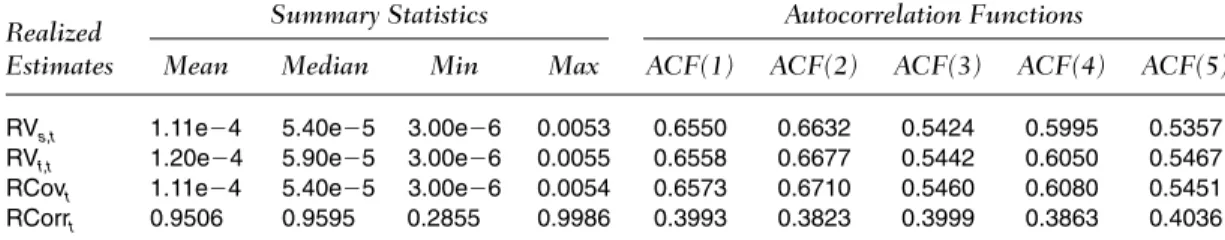
This study uses 15-minute intraday prices (m⫽ 26) to construct the real-ized (co-)variance estimates, and summarizes their descriptive statistics in Table II. As only observations during the floor trading section are sampled, the average realized variances are smaller than the corresponding unconditional variances obtained from daily returns. For example, the average value of the
RCovt(m)⫽ amj⫽1rs,tjrf,tj
amj⫽1r2i,tj
RVi,t(m)⫽
rtj⫽ p(tj)⫺p(tj⫺1)
TABLE II
Data Description: Realized Variance, Covariance, and Correlation Realized Summary Statistics Autocorrelation Functions
Estimates Mean Median Min Max ACF(1) ACF(2) ACF(3) ACF(4) ACF(5)
RVs,t 1.11e⫺4 5.40e⫺5 3.00e⫺6 0.0053 0.6550 0.6632 0.5424 0.5995 0.5357 RVf,t 1.20e⫺4 5.90e⫺5 3.00e⫺6 0.0055 0.6558 0.6677 0.5442 0.6050 0.5467 RCovt 1.11e⫺4 5.40e⫺5 3.00e⫺6 0.0054 0.6573 0.6710 0.5460 0.6080 0.5451 RCorrt 0.9506 0.9595 0.2855 0.9986 0.3993 0.3823 0.3999 0.3863 0.4036
Notes. The sample period for these (daily) realized estimates, which are constructed from fifteen-minute equidistant intraday
returns, spans the period of January 1, 1998–March 31, 2009, and the sample size is 2,828. It is noted that the futures returns after 3:00 p.m. Chicago time for each day are dropped as the futures markets close fifteen minutes later than the spot markets. The ACF(k) indicates the sample autocorrelation function of the realized estimates corresponding to lags k⫽ 1,2,. . . , 5. The upper and lower confidence bounds of the ACF with the 5% confidence level are 0.0375 and ⫺0.0375, respectively.
8The (floor) trading section for the S&P 500 index futures on the CME runs from 8:30 a.m. Chicago time
realized variance estimates for the S&P 500 cash index is 1.11e ⫺ 4, which is about 58% of the unconditional variance 1.90e ⫺ 4 calculated from Table I. To measure the realized variance (covariance) for the whole day, the squared (cross-product) overnight returns can further be incorporated into the realized estimators (De Pooter et al., 2008; Fleming et al., 2003, Hansen & Lunde, 2005; Martens, 2002). For the realized correlations, the average level for the S&P 500 (about 0.95) shows slight bias toward zero as compared with the cor-responding unconditional correlation estimates (about 0.98) using Equation (6). According to Hayashi and Yoshida (2005) and Voev and Lunde (2007), the biasness may come from the nonsynchronous trading and/or the market microstructure noise, but it can be corrected using some bias-correction tech-niques.9 The ACF of these realized estimates are also reported in Table II. It shows that these realized second moments reveal considerable persistency. However, the ACF of the realized variance (covariance) is higher than the cor-responding ACF of squared (cross-product) returns in Table I. For example, in the spot market, the ACF(1) of the realized variance is about 0.66, which is higher than the ACF(1) of the squared returns in Table I by about 0.37. We expect that the behavior difference between the realized variance (covariance) and squared (cross-product) returns should produce different volatility (covari-ance) estimates and forecasts based on the alternative and the conventional methods.
Estimation Results
Table III presents the estimation results of the return-based and the RV-based GARCH models. Panel A shows the conditional mean and variance estimates, and Panel B shows the conditional correlation estimates. Given the evidence of the cointegration relationship between the spot and futures (in Table I), the restricted ECT (St⫺1 ⫺ Ft⫺1), is parameterized in the conditional mean equa-tions to avoid the loss of long-run information; though, all a1fare insignificant different from zero (Brooks et al., 2002; Park & Switzer, 1995). The insignifi-cance of a0fand a1fcoefficients show the expected returns of futures should be zero, meaning the minimum variance hedge is generally the expected utility maximization hedge (Baillie & Myers, 1991; Kroner & Sultan, 1993).
Although the estimates of the conditional mean equations are similar, the results in the conditional variance and/or correlation equations are quite differ-ent. Concerning the result of the conventional models, the insignificance of the b2ishows the symmetric GARCH specification seems more suitable for the
9We do not adjust for the biases in the empirical analyses because the bias-correction procedures do not
data. The persistence of the GARCH for the spot and futures are about 0.9947 and 0.9933, respectively, which suggests the conditional volatilities reveal high persistence. For the correlation equations, the inferences conclude that the DCC is held. Hence, the empirical evidence using daily information indicates the ECT-GARCH-DCC model fits reasonably well to the S&P 500 market.
TABLE III
Estimation Results of RV-Based and Return-Based Models
Return-Based RV-Based
Parameters/ ECT-GARCH ECT-GJR ECT-RV-GARCH ECT-RV-GJR
Statistics CCC DCC CCC DCC CCC DCC CCC DCC
Panel A: Estimates of conditional mean and conditional variance equations
a0s ⫺1.88e⫺5 ⫺0.0004 ⫺0.0004 ⫺0.0004
(⫺0.07) (⫺1.72) (⫺1.64) (⫺1.95)
a1s ⫺0.1035 ⫺0.0880 ⫺0.0947 ⫺0.1010
(⫺2.54) (⫺2.76) (⫺2.40) (⫺2.58)
b0s 1.13e⫺6 1.31e⫺6 6.76e⫺6 4.79e⫺6
(5.91) (7.02) (7.57) (7.09) b1s 0.9173 0.9258 0.7702 0.8261 (121.28) (113.79) (33.59) (45.93) b2s 0.0774 0.0001 0.2297 0.0773 (10.68) (0.01) (9.10) (4.22) b3s – 0.1311 – 0.1929 (10.52) (7.01) a0f 0.0005 1.12e⫺5 0.0002 0.0001 (2.23) (0.05) (0.73) (0.36) a1f 0.0440 0.0065 0.0613 0.0486 (1.03) (0.19) (1.52) (1.23)
b0f 1.36e⫺6 1.45e⫺6 7.33e⫺6 5.30e⫺6
(6.99) (7.67) (8.24) (7.65) b1f 0.9121 0.9217 0.7325 0.7958 (117.37) (114.13) (28.70) (39.87) b2f 0.0812 0.0001 0.2674 0.0915 (10.98) (0.01) (9.44) (4.29) b3f – 0.1379 – 0.2251 (10.86) (7.51)
Panel B: Estimates of constant (dynamic) conditional correlation processes
u1 – 0.2537 – 0.1416 – 0.9929 – 0.9932 (3.24) (2.50) (660.87) (687.19) u2 – 0.0374 – 0.0515 – 0.0018 – 0.0018 (7.59) (8.61) (4.43) (4.49) r 苶sf(rsf) 0.9732 0.9716 0.9719 0.9700 0.9736 0.9675 0.9728 0.9667 (2821.10) (2728.50) (3036.90) (2932.00)
Notes. The entries (in the parentheses) are the Gaussian QML estimates (and their asymptotic t-statistics) of return-based and
RV-based models, where parameters are estimated via a two-step estimation method. This method first estimatesqi:⫽ (ai, bi) for i⫽ s,
f by maximizing the Gaussian quasi-likelihood function ,
then estimates u by maximizing the -based quasi-likelihood function , where ft(u) represents the
condi-tional probability density function of the standard bivariate normal distribution. LC(u0ˆ) ⫽ 1 Tg T t⫽1ln ft(eˆt; u) ˆi LVi(i)⫽ ⫺ 1 2ln 2p⫺ 1 2TgTt⫽1ln hi,t⫺ 1 2Tg T t⫽1h⫺1i,t [ri,t⫺ a0i⫺ a1i(St⫺1⫺ Ft⫺1)]2
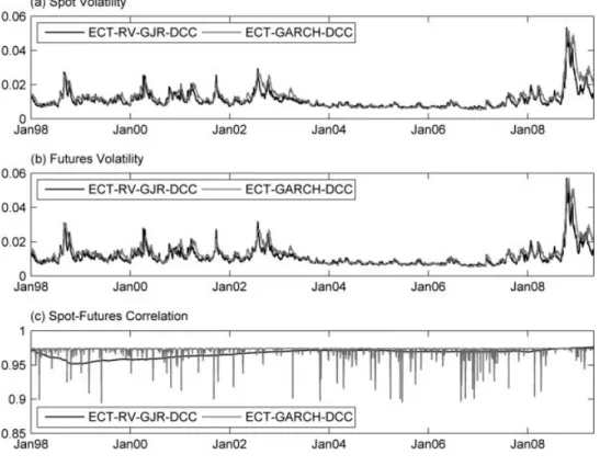
Then turn to the estimation results of the RV-based models. The significance of b3i suggests that the asymmetry in volatility are revealed. A positive b3i shows that the impact of a positive return shock on the current volatility is smaller than that of a negative return shock of the same magnitude. Particularly, the persistence of volatility implied by the RV-based models is about 0.9999, which is higher than the persistence implied by the return-based models. Besides the persistence, the weight on the persistence parameters between the two methods also differs. Taking the spot volatility as an example, the return-based GARCH estimates of b1i(b2i) is about 0.91 (0.08), whereas the RV-based GARCH esti-mates of b1i (b2i) is about 0.77 (0.23). The higher weight on the b2i using RV-based GARCH indicates that past RV may provide more information in predicting the current volatility than those using lagged daily return squares. For the conditional correlation equations, the significance of u1and u2for the S&P 500 indicates the null of mean-reverting DCC hypothesis is held. In addi-tion, the higher persistence of the RV-based correlation than the return-based one is also observed from the empirical evidence. It shows that the persistence of correlation implied by the RV-based models is about 0.99, which is much higher than the persistence (ranges from 0.19 to 0.29) implied by the return-based models. Thus, the empirical evidence using RV indicates the ECT-RV-GJR-DCC model seems suitable to the S&P 500 data. Figure 1 compares the conditional volatility and correlation estimates using the two methods. We report the best-fitted models among them to save space. It is evident that the RV-based second moment estimates are not equal to those of the return-based models. Essentially, the difference should come from the dynamics difference between the RV and the return squares.
RV-based Hedge Ratios and their Hedging Performances
We now turn to analyze the performance of a futures hedge using the RV approach. As the hedging decision has to be made ex-ante, the evaluation is conducted in an out-of-sample context using a rollover method.10To do so, this study splits the full sample period into two: the in-sample period (from January 1, 1998 to December 18, 2003; 1500 observations), and the out-of-sample period (from December 19, 2003 to March 31, 2009; 1328 observations). Each model is estimated with the use of the in-sample data and then re-estimated with a daily rollover in the out-of-sample period, keeping the estimation sample size of 1500 (fixed). This rollover method is continued for all the 1328 out-of-samples. The estimated hedge ratios as indicated in Equation (9) for each model are
subsequently constructed, and the corresponding realized portfolio returns for both the short (rp,t⫹1 ⫽ rs,t⫹1⫺ btrf,t⫹1) and the long (rp,t⫹1⫽ ⫺rs,t⫹1⫹ btrf,t⫹1) hedges are calculated. In addition to the dynamic models specified in the pre-vious sections, we also evaluate the performance of the static OLS method based on this rollover method. Particularly, to see whether the RV-based mod-els can provide a superior hedging performance during the crisis, the results before (Period I: December 19, 2003 through September 28, 2007, 950 obser-vations) and during (Period II: October 1, 2007 through March 31, 2009, 378 observations) that period are separately reported.
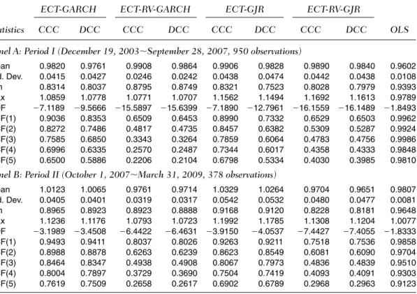
Table IV exhibits some diagnostic statistics of the hedge ratios; and, Figure 2 plots the dynamic hedge ratios.11 On average, the RV-based hedge ratios are larger (smaller) than the conventional return-based hedge ratios in Period I (II); however, they have smaller variation in both the periods. The ADF tests on the hedge ratios illustrate the unit-root hypothesis is rejected at the 5% level except
FIGURE 1
In-sample comparisons on volatility and correlation estimates: RV-based vs. return-based methods.
for the results based on the OLS (in both periods) and the ECT-GARCH-CCC (in period II) models.12The study also reports the ACF values of these out-of-sample hedge ratios up to lag five. It is apparent that, the ACF of the RV-based hedge ratios is smaller but decays more quickly than the ACF of the return-based hedge ratios.
Table V presents several statistics on the realizations of the hedged portfo-lio returns. Considering the hedging performance using standard deviation (Std. Dev.), the results show that the RV-based method yields an average sample volatility of 0.1730% (0.4284%) for the Period I (II), which is smaller than the 0.1745% (0.4404%) of the conventional method. That is, the improvement of the RV-based method over the return-based method is about 0.90 and 2.74% for the Periods I and II, respectively. Particularly, the RV-based method even can
TABLE IV
Summary Statistics of Out-of-Sample Hedge Ratios
ECT-GARCH ECT-RV-GARCH ECT-GJR ECT-RV-GJR
Statistics CCC DCC CCC DCC CCC DCC CCC DCC OLS
Panel A: Period I (December 19, 2003⬃September 28, 2007, 950 observations)
Mean 0.9820 0.9761 0.9908 0.9864 0.9906 0.9828 0.9890 0.9840 0.9602 Std. Dev. 0.0415 0.0427 0.0246 0.0242 0.0438 0.0474 0.0442 0.0438 0.0108 Min 0.8314 0.8037 0.8795 0.8749 0.8321 0.7523 0.8028 0.7979 0.9393 Max 1.0859 1.0778 1.0771 1.0707 1.1562 1.1494 1.1692 1.1613 0.9789 ADF ⫺7.1189 ⫺9.5666 ⫺15.5897 ⫺15.6399 ⫺7.1890 ⫺12.7961 ⫺16.1559 ⫺16.1489 ⫺1.8493 ACF(1) 0.9036 0.8353 0.6509 0.6453 0.8990 0.7332 0.6529 0.6503 0.9962 ACF(2) 0.8272 0.7486 0.4817 0.4735 0.8457 0.6382 0.5309 0.5287 0.9924 ACF(3) 0.7585 0.6850 0.3343 0.3264 0.7859 0.6064 0.4783 0.4756 0.9986 ACF(4) 0.6996 0.6335 0.2570 0.2487 0.7344 0.6017 0.4358 0.4333 0.9848 ACF(5) 0.6500 0.5886 0.2206 0.2104 0.6798 0.5334 0.4030 0.3985 0.9810
Panel B: Period II (October 1, 2007⬃March 31, 2009, 378 observations)
Mean 1.0123 1.0065 0.9761 0.9714 1.0329 1.0264 0.9704 0.9651 0.9807 Std. Dev. 0.0405 0.0401 0.0319 0.0317 0.0542 0.0532 0.0480 0.0477 0.0081 Min 0.8965 0.8923 0.8923 0.8888 0.9168 0.9120 0.8228 0.8181 0.9648 Max 1.1236 1.1176 1.0793 1.0723 1.1992 1.1785 1.1308 1.1204 1.0077 ADF ⫺3.1989 ⫺3.4508 ⫺6.4422 ⫺6.4631 ⫺3.9150 ⫺4.0537 ⫺7.4427 ⫺7.4055 ⫺1.8333 ACF(1) 0.9493 0.9411 0.8037 0.8026 0.9263 0.9211 0.7518 0.7536 0.9858 ACF(2) 0.8988 0.8878 0.6263 0.6239 0.8623 0.8549 0.6081 0.6090 0.9704 ACF(3) 0.8464 0.8347 0.4938 0.4908 0.8067 0.7973 0.4836 0.4839 0.9510 ACF(4) 0.8004 0.7897 0.3729 0.3690 0.7504 0.7419 0.4093 0.4091 0.9303 ACF(5) 0.7619 0.7509 0.2658 0.2617 0.6902 0.6789 0.2968 0.2963 0.9123
Notes. The ADF indicates the augmented Dickey-Fuller unit root test based on trend stationary AR model, where the 5% critical values
for Period I and II are ⫺3.4150 and ⫺3.4234, respectively. The ACF(k) indicates the sample autocorrelation function of the hedge ratios corresponding to lags k. Their 95% confidence bonds for Periods I and II are [⫺0.0649, 0.0649] and [⫺0.1029, 0.1029], respectively.
12This agrees with the finding of Lien et al. (2002), who report that the out-of-sample GARCH hedge ratios
surpass the simple OLS method during the crisis, whereas the return-based GARCH method does not.13Besides the Std. Dev., two alternatives, namely the value-at-risk (VaR) and the expected shortfall (ES), are also included in the com-parisons as the evaluation results may change if performance criteria other than traditional measures are applied (Cotter & Hanly, 2006).14The result shows that using the RV-based method generally can provide a better performance in managing portfolio VaR and ES especially during the crisis period. In addition,
FIGURE 2
Out-of-sample hedge ratios: RV-based vs. return-based methods.
13Lien et al. (2002) indicate that the out-of-sample CCC-GARCH hedge does not outperform the OLS hedge
in the S&P 500 market, where their data were extracted for the period of January 1988 through June 1998. However, Cotter and Hanly (2006) show that the CCC-GARCH hedge can beat the OLS hedge in the S&P 500 market in terms of variance reduction, where their data were extracted for the period of January 1998 through December 2003.
14The VaR is defined by the negative of the ath empirical percentile of the realizations on hedged portfolio
returns, i.e., , where denotes the empirical distribution of the hedged port-folio returns using the n realized observations. A major shortcoming with the VaR is that it is not a coherent risk measure (Artzner, Delbaen, Eber, & Heath, 1999). Hence, the ES measure has received some attention recently. The ES summarizes the negative of the average returns on the portfolio given that the hedged port-folio return has exceeded its ath empirical percentile, or , where represents the sample average operator. This gives the hedger additional information about both the probability of losses and possible magnitude of losses beyond the ath percentile.
Eˆn
ES (a)⫽ ⫺Eˆn(rpt⫹1ƒ rpt⫹1ⱕ ⫺ VaR (rpt⫹1; a))
Fˆn VaR (a)⫽⫺Fˆ⫺1
T
ABLE V
Out-of-Sample Comparisons of Hedging P
erformance: Statistical Evaluations
Short Hedge Long Hedge Std. Dev . V aR(.95) ES(.95) V aR(.99) ES(.99) V aR(.95) ES(.95) V aR(.99) ES(.99) Models (⫻ 10 ⫺ 2 )( ⫻ 10 ⫺ 2 )( ⫻ 10 ⫺ 2 )( ⫻ 10 ⫺ 2 )( ⫻ 10 ⫺ 2 )( ⫻ 10 ⫺ 2 )( ⫻ 10 ⫺ 2 )( ⫻ 10 ⫺ 2 )( ⫻ 10 ⫺ 2 ) P anel A: P eriod I (December 19, 2003 ⬃ September 28, 2007, 950 observations) ECT -GARCH-CCC 0.1753 0.2917 0.4305 0.4859 0.7269 0.2493 0.3592 0.4476 0.5557 ECT -R V -GARCH-CCC 0.1729 0.2719 0.4220 0.5037 0.7291 0.2444 0.3677 0.4781 0.6005 (⫺ 0.0024) (⫺ 0.0198) (⫺ 0.0085) (⫹ 0.0178) (⫹ 0.0022) (⫺ 0.0049) (⫹ 0.0085) (⫹ 0.0305) (⫹ 0.0448) ECT -GARCH-DCC 0.1750 0.2888 0.4280 0.4848 0.7143 0.2495 0.3591 0.4323 0.5570 ECT -R V -GARCH-DCC 0.1727 0.2719 0.4206 0.5022 0.7238 0.2461 0.3668 0.4767 0.5990 (⫺ 0.0023) (⫺ 0.0169) (⫺ 0.0074) (⫹ 0.0174) (⫹ 0.0095) (⫺ 0.0034) (⫹ 0.0077) (⫹ 0.0444) (⫹ 0.0420) ECT -GJR-CCC 0.1740 0.2830 0.4251 0.4760 0.7247 0.2498 0.3577 0.4165 0.5560 ECT -R V -GJR-CCC 0.1732 0.2699 0.4087 0.4891 0.7266 0.2563 0.3754 0.4635 0.5852 (⫺ 0.0008) (⫺ 0.0131) (⫺ 0.0164) (⫹ 0.0131) (⫹ 0.0019) (⫹ 0.0065) (⫹ 0.0177) (⫹ 0.0470) (⫹ 0.0292) ECT -GJR-DCC 0.1738 0.2860 0.4208 0.4987 0.7064 0.2494 0.3606 0.4656 0.5663 ECT -R V -GJR-DCC 0.1730 0.2700 0.4074 0.4875 0.7224 0.2553 0.3746 0.4635 0.5831 (⫺ 0.0008) (⫺ 0.0160) (⫺ 0.0134) (⫺ 0.01 12) (⫹ 0.0160) (⫹ 0.0059) (⫹ 0.0140) (⫺ 0.0021) (⫹ 0.0168) OLS 0.1719 0.2719 0.4213 0.4845 0.7059 0.2493 0.3533 0.4142 0.5526 P anel B: P eriod II (October 1, 2007 ⬃ March 31, 2009, 378 observations) ECT -GARCH-CCC 0.4378 0.6735 1.0276 1.1741 1.6902 0.7315 1.0899 1.5817 1.6778 ECT -R V -GARCH-CCC 0.4241 0.7007 1.0166 1.271 1 1.4693 0.7125 1.0128 1.2146 1.5001 (⫺ 0.0137) (⫹ 0.0272) (⫺ 0.01 10) (⫹ 0.0970) (⫺ 0.2209) (⫺ 0.0190) (⫺ 0.0771) (⫺ 0.3671) (⫺ 0.1777) ECT -GARCH-DCC 0.4367 0.6807 1.0274 1.1885 1.6829 0.7213 1.0853 1.5714 1.6599 ECT -R V -GARCH-DCC 0.4250 0.6991 1.0178 1.2924 1.4838 0.7222 1.0091 1.2231 1.4931 (⫺ 0.01 17) (⫹ 0.0184) (⫺ 0.0096) (⫹ 0.1039) (⫺ 0.1991) (⫹ 0.0009) (⫺ 0.0762) (⫺ 0.3483) (⫺ 0.1668) ECT -GJR-CCC 0.4447 0.6908 1.0240 1.2684 1.6324 0.7365 1.1332 1.4526 1.6762 ECT -R V -GJR-CCC 0.4316 0.7013 1.0646 1.2761 1.4530 0.7055 1.0194 1.1723 1.4649 (⫺ 0.0131) (⫹ 0.0105) (⫹ 0.0406) (⫹ 0.0077) (⫺ 0.1794) (⫺ 0.0310) (⫺ 0.1 138) (⫺ 0.2803) (⫺ 0.21 13) ECT -GJR-DCC 0.4425 0.6799 1.0225 1.2839 1.6275 0.7553 1.1207 1.4315 1.6574 ECT -R V -GJR-DCC 0.4328 0.7143 1.0677 1.2908 1.4654 0.7299 1.0189 1.1703 1.4510 (⫺ 0.0097) (⫹ 0.0344) (⫹ 0.0452) (⫹ 0.0069) (⫺ 0.1621) (⫺ 0.0254) (⫺ 0.1018) (⫺ 0.2612) (⫺ 0.2064) OLS 0.4357 0.6855 1.0752 1.2734 1.5828 0.7193 1.0316 1.3290 1.6004 Notes.
The values in columns Std. Dev
., V
aR, and ES are standard deviation, value-at-risk, and expected shortfall of the realized hedg
ed portfolio returns.
The entries in the
parenthe-ses are the relative values of the improvement of the alternative over the conventional hedge ratio models.
The bold values are
in Period II, the improvement of RV-based method over the conventional method tends to enlarge when the percentile has moved toward 99%. For exam-ple, on average, the improvement of long hedges in VaR(0.95), ES(0.95), VaR(0.99), and ES(0.99) is about 2.53, 8.33, 20.82, and 11.43% (the percent-age change in VaR and ES reduction), respectively; and they all can surpass the simple OLS method whereas the return-based models cannot. For the per-formance in Period I, it seems that the RV-based method is inferior to the con-ventional method. In this period, it is observed that the OLS hedge has the best performance in most of the cases. Hence, the empirical evidences conclude that the RV-based hedges are more useful than the return-based hedges in managing portfolio risk especially during the surge of volatility period.
In addition to statistical evaluations, hedgers may wish to understand the economic gains of a futures hedge using the intraday-based RV approach. As a
result, the EV, , gives an amount that the
hedger would be willing to sacrifice each day to switch from the benchmark strategy to the alternative strategy, where represents the sample average operator (Lence, 1995). Note that the mean–variance utility function EU(g)⫽
E(rp,t⫹1)⫺ gvar(rp,t⫹1) is specified with the degree of risk aversion g⬎ 0.15The advantage of using EV is that it further accounts for the hedger’s risk prefer-ence. This study considers four different levels of risk aversion g⫽ 1, 3, 7, 10 to assess the performance gains across hedgers.16 The results for each model and each period examined are summarized in Table VI.17
Table VI illustrates that the RV-based hedges can substantially outperform the static OLS and/or the return-based dynamic GARCH hedges in terms of EV gains. For short hedges in Period I, the RV-based method generates positive EV gains over the conventional and the OLS methods, whereas the EV of the return-based GARCH method over the OLS is negative. Taking g⫽ 1 as an example, the average EV of the RV-based hedges surpasses the return-based GARCH (OLS) hedges by about 0.17 (0.07) basis points per day, whereas the average EV gain of the return-based GARCH method over the OLS is about ⫺0.10 basis points per day. For long hedges, however, it is observed that the RV-based method not only underperforms the return-based GARCH method but also loses the static OLS method in Period I. As the expected hedged port-folio returns E(rp,t⫹1) for short and long hedges have the same magnitude but with opposite sign, the benefits for short hedging using RV should be harmful
Eˆn
EˆnU(rbp,t⫹1; g) ⫽ EˆnU(rap,t⫹1⫺ EV; g)
15The utility function is also considered in Kroner and Sultan (1993) and Lien and Yang (2006).
16This specification on risk aversion follows Patton (2004), who considers g⫽ 1, 3, 7, 10, 20 for asset
allo-cating. In addition, Lien and Yang (2006) assume that the risk aversion to be 4 in measuring the expected utility of a futures hedge.
17Given risk aversion g, the EV of the alternative over the benchmark model is obtained by solving the
non-linear equation: with the use of the
out-of-sample hedged portfolio returns.
E(rb
T
A
BLE VI
Out-of-Sample Comparisons of Hedging P
erformance: EV Gains Short Hedge Long Hedge Benchmark Alternative g ⫽ 1 g ⫽ 3 g ⫽ 7 g ⫽ 10 g ⫽ 1 g ⫽ 3 g ⫽ 7 g ⫽ 10 P anel A: P eriod I (December 19, 2003 ⬃ September 28, 2007, 950 observations) ECT -GARCH-CCC ECT -R V -GARCH-CCC 0.1556 0.1572 0.1604 0.1629 ⫺ 0.1539 ⫺ 0.1522 ⫺ 0.1490 ⫺ 0.1465 ECT -GARCH-DCC ECT -R V -GARCH-DCC 0.1250 0.1267 0.1299 0.1324 ⫺ 0.1234 ⫺ 0.1217 ⫺ 0.1 184 ⫺ 0.1 159 ECT -GJR-CCC ECT -R V -GJR-CCC 0.2061 0.2067 0.1926 0.1946 ⫺ 0.2056 ⫺ 0.2051 ⫺ 0.2041 ⫺ 0.2033 ECT -GJR-DCC ECT -R V -GJR-DCC 0.1754 0.1758 0.1769 0.1777 ⫺ 0.1748 ⫺ 0.1743 ⫺ 0.1732 ⫺ 0.1725 OLS ECT -R V -GARCH-CCC 0.0230 0.0223 0.0209 0.0199 ⫺ 0.0237 ⫺ 0.0243 ⫺ 0.0257 ⫺ 0.0267 OLS ECT -R V -GARCH-DCC 0.0371 0.0366 0.0356 0.0348 ⫺ 0.0376 ⫺ 0.0381 ⫺ 0.0391 ⫺ 0.0398 OLS ECT -R V -GJR-CCC 0.1009 0.1001 0.0983 0.0970 ⫺ 0.1018 ⫺ 0.1027 ⫺ 0.1045 ⫺ 0.1058 OLS ECT -R V -GJR-DCC 0.1 156 0.1 148 0.1 134 0.1 123 ⫺ 0.1 163 ⫺ 0.1 170 ⫺ 0.1 185 ⫺ 0.1 196 OLS ECT -GARCH-CCC ⫺ 0.1326 ⫺ 0.1349 ⫺ 0.1395 ⫺ 0.1430 0.1302 0.1279 0.1233 0.1 198 OLS ECT -GARCH-DCC ⫺ 0.0879 ⫺ 0.0901 ⫺ 0.0943 ⫺ 0.0976 0.0858 0.0836 0.0793 0.0761 OLS ECT -GJR-CCC ⫺ 0.1052 ⫺ 0.1066 ⫺ 0.0943 ⫺ 0.0976 0.1038 0.1024 0.0996 0.0975 OLS ECT -GJR-DCC ⫺ 0.0598 ⫺ 0.0610 ⫺ 0.0635 ⫺ 0.0654 0.0585 0.0573 0.0547 0.0529 P anel B: P eriod II (October 1, 2007 ⬃ March 31, 2009, 378 observations) ECT -GARCH-CCC ECT -R V -GARCH-CCC ⫺ 1.0951 ⫺ 1.0714 ⫺ 1.0241 ⫺ 0.9887 1.1 187 1.1423 1.1896 1.2251 ECT -GARCH-DCC ECT -R V -GARCH-DCC ⫺ 1.0760 ⫺ 1.0558 ⫺ 1.0152 ⫺ 0.9849 1.0963 1.1 166 1.1571 1.1875 ECT -GJR-CCC ECT -R V -GJR-CCC ⫺ 1.5027 ⫺ 1.4799 ⫺ 1.4340 ⫺ 1.3995 1.5257 1.5486 1.5946 1.6289 ECT -GJR-DCC ECT -R V -GJR-DCC ⫺ 1.4798 ⫺ 1.4625 ⫺ 1.4283 ⫺ 1.4025 1.4969 1.5141 1.5483 1.5740 OLS ECT -R V -GARCH-CCC ⫺ 0.2879 ⫺ 0.2678 ⫺ 0.2277 ⫺ 0.1977 0.3079 0.3279 0.3680 0.3981 OLS ECT -R V -GARCH-DCC ⫺ 0.3628 ⫺ 0.3443 ⫺ 0.3072 ⫺ 0.2795 0.3813 0.3998 0.4368 0.4646 OLS ECT -R V -GJR-CCC 0.1916 0.1987 0.2131 0.2239 ⫺ 0.1844 ⫺ 0.1772 ⫺ 0.1628 ⫺ 0.1521 OLS ECT -R V -GJR-DCC 0.1068 0.1 120 0.1222 0.1300 ⫺ 0.1017 ⫺ 0.0965 ⫺ 0.0863 ⫺ 0.0786 OLS ECT -GARCH-CCC 0.8072 0.8036 0.7964 0.7910 ⫺ 0.8108 ⫺ 0.8144 ⫺ 0.8216 ⫺ 0.8270 OLS ECT -GARCH-DCC 0.7132 0.71 15 0.7080 0.7054 ⫺ 0.7150 ⫺ 0.7168 ⫺ 0.7203 ⫺ 0.7229 OLS ECT -GJR-CCC 1.6943 1.6786 1.6471 1.6234 ⫺ 1.7101 ⫺ 1.7258 ⫺ 1.7574 ⫺ 1.7810 OLS ECT -GJR-DCC 1.5866 1.5745 1.5505 1.5325 ⫺ 1.5986 ⫺ 1.6106 ⫺ 1.6346 ⫺ 1.6526 Notes.
The table shows the basis point fees per day that an hedger with the quadratic utility and the constant relative risk aversion
of
g
would willing to pay to switch the benchmark to
the alternative strategies. Note that the ef
to the long hedge when the hedgers have the quadratic utility form. Then examining the performance in Period II, the average EV gain over the conven-tional method by the RV-based method for long (short) hedges is about 1.35 (⫺1.24) basis points per day. As compared with the OLS method, it is observed that the ECT-RV-GARCH-based (ECT-RV-GJR-based) models for long (short) hedges can generate positive EV gains in the period. Clearly, a short (long) hedger with the mean–variance utility would prefer using the RV-based method for his/her hedging activity in Period I (II). Moreover, it is evident that the EV gains of the RV-based models differentiate across hedgers with different risk aversions. The EV of the alternative method surpasses the conventional method because it increases as the risk aversion of the hedger increases. That is, a hedger with a higher risk aversion in the S&P 500 market can benefit more when he/she uses the RV-based models in hedging.
Hedge Horizon, Hedge Ratio, and Hedging Effectiveness
As we have discussed the results based on a daily hedging horizon, as individu-als and institutions may not have the same hedging horizon for their specific purposes, the RV-based method is further applied to study the effect of hedging horizon on hedge ratio and hedging effectiveness. A few studies have found that hedge ratio depends on the hedging horizon and approaches unity (i.e., naïve hedge ratio) for a longer horizon; and, hedging effectiveness tends to increase as the length of hedging horizon increases (see, for example, Chen, Lee, & Shrestha, 2004; Ederington, 1979; Geppert, 1995; Lien and Shrestha, 2007).18It is noted that, however, this result has never been examined empiri-cally using the RV-based and the return-based GARCH methods. Thus, this study analyzes the relationships of the dynamic methods for six hedging hori-zons: 1-week (1W), 2-week (2W), 3-week (3W), 1-month (1M), 2-month (2M), and 3-month (3M), and the in-sample and out-of-sample results are plotted in Panel (a)–b) and (c)–(d) of Figure 3, respectively.19Panel (a) and (c) show the hedge ratio tends to increase and to approach unity with increase of the length
18For example, the findings are supported by Ederington (1979), Geppert (1995), and Lien and Shrestha
(2007). These studies use the OLS technique, the cointegration method, and the wavelet analysis, respec-tively, to study the effect of hedging horizon length on the minimum-variance hedge ratio and the hedging effectiveness of Ederington (1979).
19Lien and Shrestha (2007) indicate that there are two ways to incorporate hedging horizon in estimating
hedge ratio. One way is to derive an optimal hedge ratio that explicitly depends on hedging horizon based on some models, such as the model of Geppert (1995). The other way is to estimate the hedge ratio by match-ing the data frequency with the hedgmatch-ing horizon, such as the approach used by Chen et al. (2004). In this study, we use the nonoverlapping approach of Chen et al. (2004) that matches the data frequency to estimate the hedge ratio and the resulting hedging effectiveness. The figures plot the average values of the empirical results based on the conventional and the alternative models mentioned in the previous sections.
of hedging horizon. For the in-sample case, the conventional hedge ratio is like-ly to exceed the alternative hedge ratio except the 3W and the 1M horizons. For the out-of-sample study, however, the alternative generally has higher hedge ratio estimates but not for the 3W and the 3M cases. In terms of hedging per-formance, Panel (b) and (d) plot the effect of hedging horizon on the hedging effectiveness as shown by Ederington (1979), which is estimated by calculating the percentage reduction in the variance of the naked spot portfolio. It is apparent that the hedging effectiveness increases with the length of hedging horizon, but the degree of hedging effectiveness does not approach one. For the out-of-sample analysis, the RV-based method generally outperforms the con-ventional method in terms of the hedging effectiveness for shorter horizons (within 2 weeks), but fail to outperform the conventional method for longer horizons.20As a result, to achieve a better hedging performance, it is suggested
FIGURE 3
The effect of hedge horizon on hedge ratio and hedging effectiveness: RV-based (solid) vs. return-based (dash) methods.
20It should be noted that, however, the sample size used to estimate hedge ratio and hedging effectiveness
decreases quickly with hedging horizon length (e.g., there are only 20 out-of-sample estimates for 3M hedg-ing horizon). Hence, the results for longer horizons, such as 2M and 3M, may not be reliable because a lower frequency results in a substantial reduction in the sample size (see, e.g., Lien & Shrestha, 2007).
that hedgers should use more futures contracts for hedging when their hedging horizon is no longer than two weeks.
CONCLUSIONS
This study has proposed a new class of RV-based GARCH models to estimate risk-minimizing hedge ratios and has examined their benefits relative to the return-based GARCH and OLS models. The RV approach, which utilizes finer information in intraday high-frequency data, provides a direct and consistent technique for estimating the latent volatility so that the spot-futures distribu-tion is quite realistic. Hence, it offers us a reliable method for estimating the risk-minimizing hedge ratio. In addition, the RV-based method is also applied to study the effect of hedge horizon on hedge ratio and hedging effectiveness, which has important implications for hedgers with different hedging horizons.
The empirical results show that the conditional variances and correlations estimates (forecasts) and the resulting hedge ratios using this RV approach are different from those generated by conventional models. Obviously, the differ-ence essentially comes from the information sets used in describing the volatil-ity dynamics. As the imperfect volatilvolatil-ity proxies in the conventional GARCH models are replaced by the accurate RV estimates, the out-of-sample compar-isons indicate that the hedging performance based on the RV-based models can be substantially improved in terms of risk reductions and EV gains as compared with competing return-based models. The results are summarized from the out-of-sample comparisons of both short and long hedgers with different levels of risk aversion using a rollover method, which spans the periods from December 19, 2003 to March 31, 2009. For longer hedging horizons, however, the effectiveness of the RV-based hedge is generally inferior to the return-based GARCH hedge. Finally, it is important to point out that the results exhibited in this study are based on 15-minute intraday prices. The hedging performance should change as the sampling frequency for calculating the RV changes. Finding the optimal sampling frequency for the RV-based hedging method is an interesting area for a further research.
BIBLIOGRAPHY
Andersen, T. G., & Bollerslev, T. (1998). Answering the skeptics: Yes, standard volatility models do provide accurate forecasts. International Economic Review, 39, 885–905.
Andersen, T. G., Bollerslev, T., Christoffersen, P. F., & Diebold, F. X. (2006). Volatility and correlation forecasting. In G. Elliot, C.W.J. Granger, & A. Timmerman (Eds.), Handbook of economic forecasting (pp. 778–878). Amsterdam: North-Holland. Andersen, T. G., Bollerslev, T., Diebold, F. X., & Labys, P. (2003). Modeling and
Artzner, P., Delbaen, F., Eber, J.-M., & Heath, D. (1999). Coherent measures of risk. Mathematical Finance, 9, 203–228.
Baillie, R. T., & Myers, R. J. (1991). Bivariate GARCH estimation of the optimal com-modity futures hedge. Journal of Applied Econometrics, 6, 109–124.
Bandi, F. M., Russell, J. R., & Zhu, Y. (2008). Using high-frequency data in dynamic portfolio choice. Econometric Reviews, 27, 163–198.
Barndorff-Nielsen, O. E., & Shephard, N. (2004). Econometric analysis of realized covariation: High frequency based covariance, regression, and correlation in finan-cial economics. Econometrica, 72, 885–925.
Blair, B. J., Poon, S.-H., & Taylor, S. J. (2001). Forecasting S&P 100 volatility: The incremental information content of implied volatilities and high-frequency index returns. Journal of Econometrics, 105, 5–26.
Bollerslev, T. (1986). Generalized autoregressive conditional heteroskedasticity. Journal of Econometrics, 31, 307–327.
Bollerslev, T. (1990). Modelling the coherence in short-run nominal exchange rates: A multivariate generalized arch model. Review of Economics and Statistics, 72, 498–505.
Brooks, C., Henry, O. T., & Persand, G. (2002). The effect of asymmetries on optimal hedge ratios. Journal of Business, 75, 333–352.
Carnero, M. A., Peña, D., & Ruiz, E. (2004). Persistence and kurtosis in GARCH and stochastic volatility models. Journal of Financial Econometrics, 2, 319–342. Chen, S.-S., Lee, C.-F., & Shrestha, K. (2004). An empirical analysis of the relationship
between the hedge ratio and hedging horizon: A simultaneous estimation of the short- and long-run hedge ratios, The Journal of Futures Markets, 24, 359–386. Choudhry, T. (2003). Short run deviations and optimal hedge ratios: Evidence from
stock futures. Journal of Multinational Financial Management, 13, 171–192. Cotter, J., & Hanly, J. (2006). Reevaluating hedging performance. The Journal of
Futures Markets, 26, 677–702.
De Pooter, M., Martens, M., & van Dijk, D. (2008). Predicting the daily covariance matrix for S&P 100 stocks using intraday data–But which frequency to use? Econometric Reviews, 27, 199–229.
Ederington, L. H. (1979). The hedging performance of the new futures markets. Journal of Finance, 34, 157–170.
Engle, R. F. (2002). Dynamic conditional correlation: A simple class of multivariate GARCH models. Journal of Business and Economic Statistics, 20, 339–350. Engle, R. F., & Granger, C. W. J. (1987). Co-integration and error correction:
Representation, estimation, and testing. Econometrica, 55, 251–276.
Fleming, J., Kirby, C., & Ostdiek, B. (2003). The economic value of volatility timing using “realized” volatility. Journal of Financial Economics, 67, 473–509.
Geppert, J. M. (1995). A statistical model for the relationship between futures con-tracts hedging effectiveness and investment horizon length. The Journal of Futures Markets, 15, 507–536.
Glosten, L. R., Jagannathan, R., & Runkle, D. E. (1993). On the relation between the expected value and the volatility of the nominal excess return on stocks. Journal of Finance, 48, 1779–1801.
Hansen, P. R., & Lunde, A. (2005). A realized variance for the whole day based on intermittent high-frequency data. Journal of Financial Econometrics, 3, 525–554.
Hayashi, T., & Yoshida, N. (2005). On covariance estimation of non-synchronously observed diffusion processes. Bernoulli, 11, 359–379.
Kroner, K. F., & Sultan, J. (1993). Time-varying distributions and dynamic hedging with foreign currency futures. Journal of Financial and Quantitative Analysis, 28, 535–551.
Lence, S. H. (1995). The economic value of minimum-variance hedges. American Journal of Agricultural Economics, 77, 353–364.
Lien, D., & Shrestha, K. (2007). An empirical analysis of the relationship between hedge ratio and hedging horizon using wavelet analysis, The Journal of Futures Markets, 27, 127–150.
Lien, D., Tse, Y. K., & Tsui, A. K. C. (2002). Evaluating the hedging performance of the constant-correlation GARCH model. Applied Financial Economics, 12, 791–798. Lien, D., & Wilson, B. K. (2001). Multiperiod hedging in the presence of stochastic
volatility. International Review of Financial Analysis, 10, 395–406.
Lien, D., & Yang, L. (2006). Spot-futures spread, time-varying correlation, and hedging with currency futures. The Journal of Futures Markets, 26, 1019–1038.
Martens, M. (2002). Measuring and forecasting S&P 500 index-futures volatility using high-frequency data. The Journal of Futures Markets, 22, 497–518.
McAleer, M., & Medeiros, M. C. (2008). Realized volatility: A review. Econometric Reviews, 27, 10–45.
Myers, R. J. (1991). Estimating time-varying optimal hedge ratios on futures markets. The Journal of Futures Markets, 11, 39–53.
Park, T. H., & Switzer, L. N. (1995). Bivariate GARCH estimation of the optimal hedge ratios for stock index futures. The Journal of Futures Markets, 15, 61–67. Patton, A. J. (2004). On the out-of-sample importance of skewness and asymmetric
dependence for asset allocation. Journal of Financial Econometrics, 2, 130–168. Tse, Y. K., & Tsui, A. K. C. (2002). A multivariate generalized autoregressive
condition-al heteroscedasticity model with time-varying correlations. Journcondition-al of Business and Economic Statistics, 20, 351–362.
Voev, V., & Lunde, A. (2007). Integrated covariance estimation using high-frequency data in the presence of noise. Journal of Financial Econometrics, 5, 68–104.