二十世紀初失蹤的台灣高齡男性

(1)

行政院國家科學委員會專題研究計畫成果報告

二十世紀初失蹤的台灣高齡男性

研究成果報告(精簡版)

計畫類別：個別型計畫編號： NSC 95-2415-H-002-014- 執行期間： 95 年 08 月 01 日至 96 年 07 月 31 日執行單位：國立臺灣大學經濟學系暨研究所計畫主持人：魏凱立計畫參與人員：碩士級-專任助理：陳嘉儀處理方式：本計畫可公開查詢

中華民國 96 年 12 月 18 日

(2)

目錄

INTRODUCTION ...1

PRIMARY HYPOTHESES TESTED ...3

HYPOTHESIS 1: THE TRADE-OFF BETWEEN WEALTH AND HEALTH SHAPED TAIWAN’S POPULATION DISTRIBUTION. ...3

HYPOTHESIS 2: A COST OF PADDY FARMING WAS A HIGHER DEATH RATE. ...4

ADDITIONAL HYPOTHESES...5

PROJECT EVALUATION AND FUTURE RESEARCH...6

TABLE ONE. MORTALITY STATISTICS FOR TAIWAN’S TWENTY COUNTIES, 1906—1908 ...7

TABLE TWO. THE RELATIONSHIP BETWEEN LAND RESOURCES AND THE DEATH RATE ...8

TABLE THREE. THE EFFECT OF PADDIES ON THE EXCESS DEATH RATIO (NO SPATIAL DUMMIES)...9

TABLE FOUR. THE EFFECT OF PADDIES ON THE EXCESS DEATH RATIO (WITH SPATIAL DUMMIES)...10

(3)

Introduction

Part of my NSC project concerned inputting fine cross-sectional data (2933 villages, 小庄) from early Japanese-era Taiwan and making this data available. The data is now on my website. The data consists of (1) the almost complete 1915 census, (2) the almost complete 1920 census, (3) the land survey of 1906 and its revision in 1919 and (4) the 1906—1920 annual population reports showing deaths, births, in-migration and out-migration for each village. Dummy variables are also shown which allow each village to be placed in the proper 1901-1909 counties (廳), 1909-1920counties (廳), the pre-1920 townships (堡 and 里) or the post-1920 prefectures (州), 郡 and 大庄. Some basic geographic data was added, e.g. whether the village was on the coast or whether it was on the frontier.

My project’s hypothesis was that the high death rate for males was due to overwork. This hypothesis was suggested by the fact that the census showed a particular dearth of males in 閩南 areas as opposed to Hakka (客家) areas and in areas dominated by paddies as opposed to dry field areas. Statistics show that Taiwanese women were more likely to be in the work force in 客家 areas and in areas with dry fields. 閩南 women were more likely to be secluded and bound-footed and paddy labor was almost completely a male activity. Once I had completed the data set, I could not find clear support for my original hypothesis. The dearth of males in paddy-dominated areas and in the 閩南 area could be explained by the overall high death rates in these areas. Both men and women died earlier in these regions. Women seem to naturally live longer than men and, as a greater proportion of the population dies off, the ratio of women to men rises. It is possible that the seclusion of women from the workforce raised the death rate for both men and women but it was not possible to prove this hypothesis. The focus of my project thus changed to understanding the high Taiwanese death rate through the micro-data set I had created. Table one shows regional mortality figures for Taiwan in 1906-1908. This table was calculated from the age-specific population figures in the 1905 census and the age-specific death statistics and birth statistics in the 1906—1908 動態人口調查. The figures in the table show, (1) life expectancy at birth, (2) the chance of a child living until the age of 12, (3) the chance of a 12-year-old living to the age of 45 and (4) the chance of a 45-year-old living to the age of 65. The northern 客家 area—桃園廳, 新竹廳 and 苗栗廳—generally showed the highest life expectancies. As one moves south of this area, life expectancy drops greatly. This may be due to climate. The general spatial pattern shown in table one continues at least into the 1930s. The one area of the south which was comparatively healthy was the very southern tip of the island that had been opened up to Han immigrants comparatively recently. The

(4)

main difference between north and south was in the adult death rate. The death rate for children in the south was higher than in the north, but the difference was comparatively small. The differential in male and female life expectancy was greater in the north than in the south, but this is mainly an artifact of the high southern death rate. In short, the female advantage comes from the fact that females age slower than males, but in the south many fewer people lived long enough for the natural aging process to have any effect. One should note that even in the north, the death rate is extremely high. The Taiwanese mortality statistics for this period are of great value because they are the only detailed death statistics available for a population with such a high death rate.1 The data shown for 臺東廳 and 澎湖廳 are somewhat incomplete. In the case of 澎湖, many of the healthy working-age men seem to have been away from the island when the census was taken. This research will focus on Taiwan’s west coast and ignore these two more problematic areas.

Not only are there large regional differences across counties, but there are also large differences in village death rates within each county. The focus of this research is on the inter-villages differences in the death rate. Unfortunately, only the total number of deaths is reported for each village (and in 1915 and 1920, only the deaths during the last three months of the year are reported). Crude death rates are thus readily calculated, but there is substantial variation in the age structure of village-level populations. Thus a high crude death rate may just reflect the fact that the village has many old people and young children who have a higher probability of death.

This paper adjusts for this problem by using the village-level age categories reported in the 1915 census. In this census (and in the 1920 census) Taiwanese residents of each sex are divided into seven age categories: (1) age 0 to 4, (2) age 5 to 9, (3) age 10 to 14, (4) age 15 to 19, (5) age 20 to 49, (6) age 50 to 59 and (7) age 60 and over. I use the detailed county-level age-specific data to calculate the expected death rates for each age group in an area and then calculate the expected number of deaths given the age composition of the village. Then I divide the actual number of deaths by the expected number of deaths (instead of dividing the actual number of deaths by the total population as is done in calculating a crude death rate). I will call this number, the excess death ratio. Thus, an excess death ratio of 1 means that the number of deaths in the village was just what one would expect given the county and the village’s population and age composition. A ratio of 1.2 means that there were 20% more deaths than expected given the village’s population and age composition.

The census for 1915 was taken on October 1 and, for some reason, village data on

1

In 2007, the country with the lowest life expectancy on the planet was Swaziland with a life expectancy of 32.2 years, followed by Angola with 37.6. Taiwan’s life expectancy as shown in table one was 28.7 years

(5)

deaths, births and migration for this year are only reported for the post-census period (10/1 to 12/31). Using 3 months of data or even a year of data means accepting a lot of random variation. Using data averaged over several years gives a better picture of the village’s long-term death rate. However, the more distant the data is from the census year in terms of time, the less representative will be the 1915 age structure. This research uses the average death rate for the five-year period 1913 to 1917, less the nine unreported months in 1915.

Primary Hypotheses Tested

Hypothesis 1: The trade-off between wealth and health shaped Taiwan’s population distribution.

Taiwan was an agricultural island. By far the most important complement to human labor was improved agricultural land. People tended to live where improved agricultural land was most abundant. However, much of this land was in unhealthy areas with high death rates. If mobility costs were not prohibitive, all other things being equal, one would expect farmers to reside in unhealthy areas only if this allowed them access to more or better land. These should thus be a positive correlation between land resources per person and the death rate the farm community faced.

To test this hypothesis, I examine the correlation between the excess death ratio and land resources. In the 1919 land survey, the Japanese authorities estimated how much harvest the land in each village would yield (in yen). The 1915 census reported the number of people in the village working in agriculture or relying on those working in agriculture. I use the estimated harvest divided by this agriculture population as the measure of land resources. Land resources per person were somewhat greater in the south than in the north which is in accord with the hypothesis. For convenience, land resources in each village in each county are regressed on the excess death ratio, but causation runs both ways. Nine individual regressions are run showing the correlation between land resources and the excess death ratio across villages within the nine west coast 1915 counties. These results are shown in table two. The results show that in the north of the island, the expected relationship does not hold. But there is a strong positive correlation between the excess death ratio and land resources in the south where the death rate was highest and a weaker, but significant positive correlation in the middle part of the island. One finds the same result if one combines the villages together into the post-1920 大庄 and runs two regressions using these larger units: a regression for the north of the island and one for

(6)

the south. This is unexpected because there was much more emigration between villages in the north than in the south. To check if the 1915 situation was in equilibrium, I ran regressions to check if there was significant net in-migration to villages with low excessive death ratios and abundant land resources. There was no significant in-migration so the situation would seem to be an equilibrium. Since some areas had many absentee landlords, I also looked at the effect of land resources after subtracting the estimated rent to the landholders, but this did not change the basic results.

Hypothesis 2: A cost of paddy farming was a higher death rate.

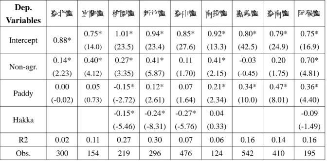
Taiwanese wage statistics show that there was a wage premium for working in paddies. Other researchers have suggested that paddy farming may be unhealthy. To test this hypothesis, I regress the excess death ratio on the proportion of the population involved in paddy farming and, as control variables, the proportion of the population in non-farming occupations and the proportion of the population that was Hakka. The proportion of the population that is agricultural can be calculated from the 1915 census and the proportion of farmland that is paddy can be calculated from the 1919 land survey. With these two numbers, I know the proportion of the population in non-agricultural occupations and I can estimate the proportion of the agricultural population in paddy agriculture by assuming the agricultural population is split between paddy agriculture and dry field agriculture in the same proportion as the land. The 1915 census also gives the proportion of the population in each village that is Hakka. Including a Hakka variable is important in some counties because, as table one suggests, the Hakka in the north of Taiwan lived longer than other Taiwanese and they tended to live in uplands with more dry farming. I left out the Hakka variable in counties in which one percent of the population or less were Hakka. Once again, I ran nine separate regressions for each of the 1915 counties in western Taiwan. The results are shown in table three. In table four the same regression is shown run with dummy variables representing each of the post-1920 大庄 to deal with spatial correlation. Coefficients for the spatial dummy variables are not shown. The results show that in the south, paddy farming was associated with a high death rate. In the north, there was no such association. Possibly the southern climate made paddies deadly, but there could also be other cultural or geographic causes. The fact that northern Hakka areas had lower death rates even after controlling for spatial correlation suggests that culture may have been an important factor. Using data from the 基本農業調查, vol. 10 (土地利用調查), I have tried to control for the

(7)

various types of irrigation used, but this does not help explain regional differences. Neither does there appear to be much difference in the reported causes of death between paddy and dry areas (衛生調查書, vol. 5, 臺灣死因統計). Females seldom worked in paddies, but male and female death rates are equally affected. Therefore, it is not working in the paddies per se that causes the high death rate. The cause would seem to be environmental. One possibility is that in southern paddy regions people tended to live in more compact villages where disease and sanitation problems would be more severe. In dry areas, farmers may have spread out more. Since housing land was also taxed (and thus surveyed) I may be able to test this hypothesis once I get more data entered. There tends to be more land resources per person in paddy areas, so one might suspect that deaths were higher in paddy areas simply because of the land-resources-health trade-off, but controlling for land resources does not significantly alter the result shown.2

Additional Hypotheses

My earlier research showed that fishermen were, on average, taller than the rest of the population. Assuming this was due to good health, I would assume that they would live longer. The 1920 census listed the number of fishermen in each village. Fishermen did live longer down south, but not in the north. The north coast of Taipei was one of the least healthy areas of the island. I also examined whether people lived longer in villages with fish ponds. I found, once again, that this was true in the south but not in the north. This suggests that southerners may have lacked protein , but areas in which livestock or poultry were raised did not show any difference in death rates.

I also used 1920 census data to see whether miners had relatively high death rates. I found that villages with miners did not have significantly higher death rates and in some areas the death rates were significantly lower than the death rates for farmers.

Generally, and particularly in the north, death rates were highest for non-agricultural workers and their dependents. Further research showed that men working in non-agricultural occupations had high death rates, but this was not necessarily true of their dependents. I tried to examine further which type of non-agricultural occupations seemed to have the highest death rate and was surprised to find that high death rates were most closely associated to villages with a greater number of people in commercial occupations (商業). However, it isn’t clear whether merchants really

(8)

had higher death rates or whether communicable diseases were simply more prevalent in areas which were more commercialized.

Project Evaluation and Future Research

This report is late because I am still working on this project. Entering the data took longer than expected. I am still entering some geographic variables into the data set which will hopefully sharpen the results. Thus far, results are interesting enough that they need further study, but more work is necessary before a publishable paper can be written. Next semester I will be giving a couple talks on this material to help me organize it into publishable form. I will also begin looking at local changes in the death rate to identify in which type areas health was improving fastest. I am also examining medical reports from the Japanese-colonial-era in an attempt to find new leads as to why southern paddy areas had high death rates.

(9)

Table One. Mortality Statistics for Taiwan’s Twenty Counties, 1906—1908 Life Expectancy (Years) Chance of Reaching Age 12 (%) Chance of Reaching Age 45, Conditional on Reaching Age 12 (%) Chance of Reaching Age 45, Conditional on Reaching Age 12 (%) 1901-1909 County 廳男女男女男女男女臺北廳 31.8 34.1 65.2 63.5 55.3 64.4 37.3 53.9 基隆廳 32.7 35 66.8 63.5 56.2 66.8 32.8 56.0 宜蘭廳 32.3 35.6 66.4 64.2 56.8 67.2 29.2 57.7 深坑廳 34.5 36.6 71.6 64.4 54.8 70.2 35.1 57.6 桃園廳 38.7 40.3 74.3 69.4 64.0 73.6 43.0 60.7 新竹廳 37.9 40.7 72.8 73.1 63.1 70.5 44.0 55.1 苗栗廳 34.4 36.6 69.5 66.8 58.7 67.1 32.9 53.7 臺中廳 28.7 33.0 62.0 63.3 49.8 61.7 23.5 45.1 彰化廳 26.2 27.6 57.9 54.4 45.2 57.6 19.0 40.2 南投廳 28.2 30.5 60.8 58.1 49.1 62.7 25.1 44.3 北部 31.8 34.4 65.9 63.7 54.5 65.2 31.4 51.1 斗六廳 25.8 26.7 59.1 56.9 41.2 48.7 18.8 33.9 嘉義廳 21.5 21.0 53.2 50.3 31.4 35.6 13.6 23.5 鹽水港廳 25.4 24.8 59.7 55.5 38.0 42.8 18.7 32.7 臺南廳 26.2 27.3 60.9 58.4 39.7 48.8 19.1 35.9 番薯寮廳 23.8 25.6 53.2 51.8 44.5 53.8 19.9 42.2 鳳山廳 23.8 24.6 58.1 56.0 33.3 42.5 14.8 26.9 阿猴廳 22.9 23.9 55.5 53.2 33.3 43.1 12.3 26.3 恆春廳 31.0 31.9 64.6 61.2 53.7 64.9 25.7 35.8 南部 24.4 24.8 57.8 55.1 36.8 44.1 16.7 30.5 臺東廳 26.4 28.3 57.6 58.0 48.7 54.9 22.4 36.3 澎湖廳 31.4 28.8 61.6 53.5 62.1 63.8 38.6 51.1 全台灣 28.0 29.3 61.8 59.4 46.2 54.9 24.8 41.0

(10)

Table Two. The Relationship Between Land Resources and the Death Rate 1915 County 廳 Land Resources mean (yen per person) Regression

Coefficient T-statistic R-squared Observations

臺北廳 37.5 1.24 0.16 0.000 252 宜蘭廳 51.3 0.14 0.01 0.000 142 桃園廳 45.6 -4.69 -0.82 0.003 204 新竹廳 35.4 16.7 3.32 0.038 278 臺中廳 53.1 26.5 3.45 0.026 450 南投廳 29.3 12.0 2.39 0.046 119 嘉義廳 43.4 55.0 8.96 0.134 521 臺南廳 71.1 128.0 6.32 0.092 398 阿猴廳 49.2 101.0 9.03 0.304 189

(11)

Table Three. The Effect of Paddies on the Excess Death Ratio (no spatial dummies) Dep. Variables 臺北廳宜蘭廳桃園廳 新竹廳臺中廳南投廳 嘉義廳臺南廳阿猴廳 Intercept 0.88* 0.75* (14.0) 1.01* (23.5) 0.94* (23.4) 0.85* (27.6) 0.92* (13.3) 0.80* (42.5) 0.79* (24.9) 0.75* (16.9) Non-agr. 0.14* (2.23) 0.40* (4.12) 0.27* (3.35) 0.41* (5.87) 0.11 (1.70) 0.41* (2.15) -0.03 (-0.45) 0.20 (1.75) 0.70* (4.81) Paddy 0.00 (-0.02) 0.05 (0.73) -0.15* (-2.72) 0.12* (2.61) 0.07 (1.64) 0.21* (2.34) 0.34* (10.0) 0.47* (8.01) 0.36* (4.40) Hakka -0.15* (-5.46) -0.24* (-8.31) -0.27* (-5.76) 0.04 (0.33) -0.09 (-1.49) R2 0.02 0.11 0.27 0.30 0.07 0.06 0.16 0.14 0.16 Obs. 300 154 219 296 476 124 542 410 195

(12)

Table Four. The Effect of Paddies on the Excess Death Ratio (with spatial dummies) Dependent Variables 臺北廳 宜蘭廳 桃園廳 新竹廳 臺中廳 南投廳 嘉義廳 臺南廳 阿猴廳 Intercept 0.81* (6.34) 0.68* (11.8) 1.05* (13.5) 1.29* (9.44) 0.66* (11.9) 0.86* (7.82) 0.89* (18.1) 1.30* (12.3) 0.62* (5.58) Non-agr. 0.20* (3.03) 0.21 (1.75) 0.34* (4.13) 0.41* (5.54) 0.19* (2.73) 0.28 (1.63) 0.03 (0.42) 0.03 (0.28) 0.62* (4.06) Paddy -0.01 (-0.11) -0.02 (-0.22) -0.15* (-2.30) 0.12* (2.15) 0.10* (2.21) 0.51* (4.49) 0.20* (4.76) 0.15* (1.98) 0.33* (3.50) Hakka -0.26* (-3.44) -0.29* (-5.18) -0.06 (-0.69) 0.28 (1.72) -0.10 (-1.31) R-squared 0.41 0.26 0.44 0.46 0.51 0.40 0.48 0.43 0.42 Observations 300 154 219 296 476 124 542 410 195

T statistics in parentheses. * indicates significance at the 95% level. ** indicates significance at the 99% level

(13)

參考文獻

Kelly B. Olds (2003), “The Biological Standard of Living in Taiwan under Japanese Occupation.” Economics and Human Biology (SSCI / EI), 2:187-206.

魏凱立 (2000), “身高與台灣人經濟福利的變化, 1854-1910” 經濟論文叢刊 (TSSCI / EI), 28:25-42 臨時臺灣戶口調查部（1907）。明治 38 年臨時台灣戶口調查要計表。臨時臺灣戶口調查部（1907）。明治 39 年臺灣現住人口統計。臺灣總督府官房統計課（1908 ~ 1917）。明治 40 年~大正 5 年臺灣現住人口統計。臺灣總督府官房調查課（1918 ~ 1922）。大正 6 年~9 年臺灣現住人口統計。臺灣總督府官房統計課（1917）。大正四年第二次臨時臺灣戶口調查概覽表。臺灣總督府官房臨時國勢調查課（1922）。大正九年第一回臺灣國勢調查(第三次臨時臺灣戶口調查)要覽表。臨時臺灣土地調查局（1905）。田收穫及小租調查書。臨時臺灣土地調查局（1905）。(火田)收穫及小租調查書。臺灣總督府財務局（1920）。臺灣地租等則修正事業成績報告書五冊ノ內 3。臨時臺灣戶口調查部（1907）。明治 39 年臺灣人口動態統計(原表之部)。臺灣總督府官房統計課（1909 ~ 1910）。明治 40~41 年臺灣人口動態統計(原表之部)。臺灣總督府警務局衛生課（1925）。衛生調查書基本調查の 5《臺灣死因統計(總數の部)》。日本福岡縣內務部第五課（1925）。臺灣農事調查書《第十土地利用調查》。

二十世紀初失蹤的台灣高齡男性

行政院國家科學委員會專題研究計畫 成果報告