An ART-Based Fuzzy Adaptive
Learning Control Network
Cheng-Jian Lin,
Member, IEEE, and Chin-Teng Lin,
Member, IEEEAbstract—This paper addresses the structure and an associated
on-line learning algorithm of a feedforward multilayered connec-tionist network for realizing the basic elements and functions of a traditional fuzzy logic controller. The proposed fuzzy adaptive learning control network (FALCON) can be contrasted with the traditional fuzzy logic control systems in their network structure and learning ability. An on-line structure/parameter learning algorithm called FALCON-ART is proposed for constructing the FALCON dynamically. It combines the backpropagation learning scheme for parameter learning and the fuzzy ART algorithm for structure learning. The FALCON-ART has some important features. First of all, it partitions the input state space and output control space using irregular fuzzy hyperboxes according to the distribution of training data. In many existing fuzzy or neural fuzzy control systems, the input and output spaces are always partitioned into “grids.” As the number of input/output variables increases, the number of partitioned grids will grow combinatorially. To avoid the problem of combinatorial growing of partitioned grids in some complex systems, the FALCON-ART partitions the input/output spaces in a flexible way based on the distribution of training data. Second, the FALCON-ART can create and train the FALCON in a highly autonomous way. In its initial form, there is no membership function, fuzzy partition, and fuzzy logic rule. They are created and begin to grow as the first training pattern arrives. Thus, the users need not give it any a priori knowledge or even any initial information on these. More notably, the FALCON-ART can on-line partition the input/output spaces, tune membership functions, find proper fuzzy logic rules, and annihilate redundant rules dynamically upon receiving on-line incoming training data. Computer simulations have been conducted to illustrate the performance and applicability of the proposed system.
Index Terms—Adaptive vector quantization, fuzzy ART, fuzzy
clustering, fuzzy hyperbox, rule annihilation, time-series predic-tion.
I. INTRODUCTION
B
RINGING the learning abilities of neural networks to automate and realize the design of fuzzy logic control systems has recently become a very active research area [1]–[18]. This integration brings the low-level learning and computation power of neural networks into fuzzy logic sys-tems and provides the high-level human-like thinking and reasoning of fuzzy logic systems into neural networks. Such synergism of integrating neural networks and fuzzy logicManuscript received March 8, 1994; revised December 12, 1996. This work was supported by the R.O.C. National Science Council under Grant NSC86-2212-E-009-019.
The authors are with the Department of Control Engineering, National Chiao-Tung University, Hsinchu, Taiwan, R.O.C.
Publisher Item Identifier S 1063-6706(97)04832-7.
into a functional system provides a new direction toward the realization of intelligent systems for various applications.
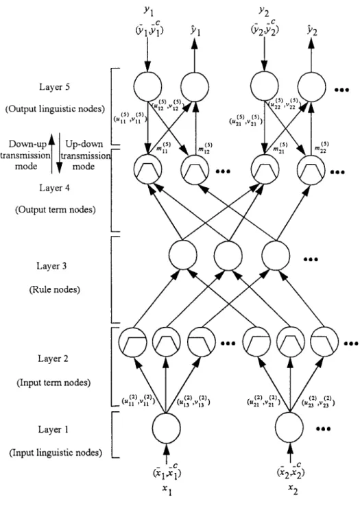
In this paper, we are extending our previous work on neural network-based fuzzy logic control systems [19] to the on-line supervised learning problems. The proposed fuzzy adaptive learning control network (FALCON) can be constructed au-tomatically by learning from training examples. It can be contrasted with the traditional fuzzy logic control systems in their network structure and learning ability. The FALCON is a five-layer structure, as shown in Fig. 1. Nodes at layer one are input nodes (linguistic nodes), which represent input linguistic variables. Layer five is the output layer. We have two linguistic nodes for each output variable. One is for training data (desired output) to feed into this net and the other is for decision signal (actual output) to be pumped out of the net. Nodes at layers two and four are term nodes, which act as membership functions to represent the terms of the respective linguistic variable. Each node at layer three is a rule node which represents one fuzzy logic rule. Thus, all layer-three nodes form a fuzzy rule base. Layer-three links define the preconditions of the rule nodes and layer-four links define the consequents of the rule nodes. The links at layers two and five are fully connected between linguistic nodes and their corresponding term nodes.
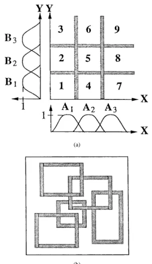
Associated with the FALCON is an on-line learning algo-rithm called FALCON-ART. We shall call a FALCON with this on-line learning algorithm the FALCON-ART model. The FALCON-ART has some important properties, as described below. In many existing fuzzy or neural fuzzy control systems, the input and output spaces are partitioned into “grids.” Each grid defines a fuzzy region and the overlapping region between the grids provides a smooth and continuous membership output surface. For example, consider a fuzzy logic controller with two input variables. If each of them contains three fuzzy terms (e.g., “small,” “medium,” and “large”), then the corresponding input space partition is as shown in Fig. 2(a). Although during the learning process, the position and shape of membership functions will be changed, they are still grid-type partitions inherently. The grid-type space partitioning of input and output spaces has been widely used in many existing fuzzy systems. It certainly makes both the fuzzy logic controller software emulation and fuzzy chip implementation convenient. However, as the number of input/output variables increases, the number of the partitioned grids will grow combinatorially. As a result, the required size of memory or hardware may become impractically huge. This results in more difficulty in learning because finer space partitioning needs more training samples; otherwise, insufficient learning will occur.
Fig. 1. Proposed FALCON.
To avoid the problem of combinatorial growing of parti-tioned grids in complex systems, more flexible and irregular space partitioning methods must be developed. Fig. 2(b) shows a proposed partitioning method in the FALCON-ART. The problem of space partitioning from numerical training data is basically a clustering problem. The proposed FALCON-ART applies the fuzzy adaptive resonance theory (fuzzy FALCON-ART) proposed by Carpenter et al. [22], [23] to do fuzzy cluster-ing in the input/output spaces and find proper fuzzy logic rules dynamically by associating input clusters and output clusters. The backpropagation learning scheme is then used for tuning input/output membership functions. Hence, the FALCON-ART combines the backpropagation algorithm for parameter learning and the fuzzy ART for structure learning.
The FALCON-ART can, thus, on-line partition the input/output spaces, tune membership functions, and find proper fuzzy logic rules dynamically in the fly. More notably, in this learning method, only the training data need to be provided from the outside world. The users need not give the initial fuzzy partitions, membership functions, and fuzzy logic rules. Hence, there is no input/output term nodes and no rule nodes in the beginning of learning. They are created dynamically as learning proceeds upon receiving on-line incoming training data.
This paper is organized as follows. Section II describes the structure of the FALCON-ART model. The on-line structure/parameter learning algorithm FALCON-ART, which combines fuzzy ART with backpropagation, is presented
(a)
(b)
Fig. 2. (a) Grid-type fuzzy partitioning. (b) Flexible hyperbox fuzzy parti-tioning.
in Section III. The structure learning consists of three learning processes: input fuzzy clustering process, output fuzzy clustering process, and mapping process. Section IV describes the proposed rule annihilation methods used in the learning process. In Section V, the FALCON-ART model is used to identify the nonlinear dynamic system, predict the Mackey–Glass chaotic time-series, control the truck backer-upper, and control the ball and beam system to demonstrate its on-line learning capability. Section VI describes the features of the proposed FALCON-ART model. Conclusions are summarized in the last section.
II. THESTRUCTURE OF THE FALCON-ART MODEL In this section, we shall describe the structure and functions of the proposed FALCON-ART model. The FALCON (see Fig. 1) has five layers with node and link numbering defined by the brackets on the right-hand side of the figure. Layer-1 nodes are input nodes (input-linguistic nodes) representing input-linguistic variables. Layer-5 nodes are output nodes (output-linguistic nodes) representing output linguistic vari-ables. Layer-2 and Layer-4 nodes are term nodes that act as membership functions representing the terms of the respective input- and output-linguistic variables. Each Layer-3 node is a rule node representing one fuzzy logic rule. Thus, together,
all the Layer-3 nodes form a fuzzy rule base. Links between Layers 3 and 4 function as a connectionist inference engine. Layer-3 links define the preconditions of the rule nodes and Layer-4 links define the consequents of the rule nodes. Therefore, each rule node has at most one link to some term node of a linguistic node, and may have no such links. This is true both for precondition links (links in Layer 3) and consequent links (links in Layer 4). The links in Layers 2 and 5 are fully connected between linguistic nodes and their corresponding term nodes. The arrows indicate the normal signal flow directions when the network is in operation (after it has been built and trained). We shall later indicate the signal propagation layer-by-layer, according to the arrow direction.
The FALCON uses the technique of complement
cod-ing from fuzzy ART [22] to normalize the input/output
training vectors. Complement coding is a normalization process that rescales an -dimensional vector in ,
, to its 2 -dimensional complement coding form in , , such that
(1)
where and is the
complement of , i.e., . As mentioned in
[22], complement coding helps avoid the problem of category proliferation when using fuzzy ART for fuzzy clustering. It also preserves training vector-amplitude information. In applying the complement coding technique to the FALCON, all training vectors (either input state vectors or desired output vectors) are transformed to their complement coded forms in the preprocessing process and the transformed vectors are then used for training.
A typical neural network consists of nodes with some finite number of fan-in connections from other nodes represented by weight values and fan-out connections to other nodes. Associated with the fan-in of a node is an integration function which combines information, activation, or evidence from other nodes, and provides the net input, i.e.,
net-input
(2)
where is the th input to a node in layer and is the weight of the associated link. The superscript in the above equation indicates the layer number. This notation will also be used in the following equations. Each node also outputs an activation value as a function of its net-input
output (3)
where denotes the activation function. Next, we shall describe the functions of the nodes in each of the five layers of the FALCON. Assume that the dimension of the input space is and that of the output space is .
Layer 1: Each node in this layer is called an input-linguistic
node and corresponds to one input-linguistic variable. Layer-1 nodes just transmit input signals to the next layer directly. That is
and
(4) From the above equation, the link weight in Layer 1 is unity. Notice that due to the complement coding process, for each input node there are two output values and
.
Layer 2: Nodes in this layer are called input-term nodes
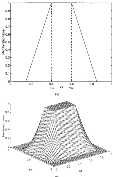
and each represents a term of an input-linguistic variable and acts as a one-dimensional (1-D) membership function. The following trapezoidal membership function [24] is used:
and
(5) where and are, respectively, the left-flat and right-flat points of the trapezoidal membership function of the th input-term node of the th input-linguistic node [see Fig. 3(a)], is the input to the th input-term node from the th input-linguistic node (i.e., ), and
if if if
(6) The parameter is the sensitivity parameter that regulates the fuzziness of the trapezoidal membership function. A large means a more crisp fuzzy set, and a smaller makes the fuzzy set less crisp. A set of input-term nodes (one for each input-linguistic node) is connected to a rule node in Layer 3 where its outputs are combined. This defines an -dimensional membership function in the input space with each dimension specified by one term node in the set. Hence, each input-linguistic node has the same number of term nodes. That is, each input-linguistic variable has the same number of terms in the FALCON. This is also true for output-linguistic nodes. A Layer-2 link connects an input-linguistic node to one of its term nodes. There are two weights on each Layer-2 link. We denote the two weights on the link from input node (corresponding to the input-linguistic variable ) to its th term node as and (see Fig 1). These two weights define the membership function in (5). The two weights and correspond, respectively, to the two inputs and from the input-linguistic node . More precisely, and , the two inputs to the input-term node , will be used during the fuzzy-ART clustering process in FALCON’s structure-learning step to decide and , respectively. In FALCON’s parameter-learning step and normal operating, only is used in the forward reasoning process [i.e., in (5)]. We detail the FALCON learning scheme in Section III.
(a)
(b)
Fig. 3. (a) One-dimensional (1-D) trapezoidal membership function. (b) Two-dimensional (2-D) trapezoidal membership function.
Layer 3: Nodes in this layer are called rule nodes and each
represents one fuzzy logic rule. Each Layer-3 node has input-term nodes fed into it, one for each input-linguistic node. Hence, there are as many rule nodes in the FALCON as there are term nodes of an input-linguistic node (i.e., the number of rules equals the number of terms of an input-linguistic variable). Notice that each input-linguistic variable has the same number of terms in the FALCON, as mentioned in the above. The links in Layer 3 are used to perform precondition matching of fuzzy logic rules. Hence, the rule nodes perform the product operation
and
(7) where is the th input to a node in Layer 3 and the product is over the inputs of this node. The link weight in Layer 3 is then unity. Note that the product operation in the above equation is equivalent to defining a multidi-mensional ( -dimultidi-mensional) membership function, which is the
product of the trapezoid functions in (5) over . This forms a multidimensional trapezoidal membership function called the
hyperbox membership function [24] since it is defined on a
hyperbox in the input space. The corners of the hyperbox are decided by the Layer-2 weights and for all ’s. More clearly, the interval defines the edge of the hyperbox in the th dimension. Hence, the weight
vector defines
a hyperbox in the input space. An illustration of a 2-D hyperbox membership function is shown in Fig. 3(b). The rule nodes output are connected to sets of output-term nodes in Layer 4, one for each output-linguistic variable. This set of output-term nodes defines an -dimensional trapezoidal (hyperbox) membership function in the output space that specifies the consequent of the rule node. Note that different rule nodes may be connected to the same output hyperbox (i.e., they may have the same consequent), as is shown in Fig. 1.
Layer 4: The nodes in this layer are called output-term
nodes; each has two operating modes: down–up transmission and up–down transmission modes (see Fig. 1). In down–up transmission mode, the links in Layer 4 perform the fuzzy OR operation on fired (activated) rule nodes that have the same consequent
and
(8) where is the th input to a node in Layer 4 and is the number of inputs to this node from the rule nodes in Layer 3. Hence, the link weight . In up–down transmission mode, the nodes in this layer and the up–down transmission links in Layer 5 function exactly the same as those in Layer 2: each Layer-4 node represents a term of an output-linguistic variable and acts as a 1-D member-ship function. A set of output-term nodes (one for each output-linguistic node) defines an -dimensional hyperbox (membership function) in the output space and there are also two weights and on each of the up–down transmission links in Layer 5 (see Fig. 1). The weights define hyperboxes (and, thus, the associated hyperbox membership functions) in the output space. More clearly, the weight
vec-tor , defines a
hyperbox in the output space.
Layer 5: Each node in this layer is called a output-linguistic
node and corresponds to one output-linguistic variable. There are two kinds of nodes in Layer 5. The first kind of node performs up–down transmission for training data (desired outputs) to feed into the network, acting exactly like the input-linguistic nodes. For this kind of node we have
and
(9)
where is the th element of the normalized desired output vector. Notice that complement coding is also performed on the desired output vectors. Thus, as mentioned above, there are two weights on each of the up–down transmission links in Layer 5 (the and shown in Fig. 1). The weights define hyperboxes and the associated hyperbox membership functions in the output space. The second kind of node performs down–up transmission for decision signal output. These nodes and the Layer-5 down–up transmission links attached to them act as a defuzzifier. If and are the corners of the hyperbox of the th term of the th output-linguistic variable , then the following functions can be used to simulate the
center of area defuzzification method:
and
(10)
where is the input to the th output-linguistic node from
its th term node and denotes the center
value of the output membership function of the th term of the th output-linguistic variable. The center of a fuzzy region is defined as that point with the smallest absolute value among all the other points in the region at which the membership value is equal to one. Here, the weight on a down–up transmission
link in Layer 5 is defined by ,
where and are the weights on the corresponding up–down transmission link in Layer 5.
The fuzzy reasoning process in the FALCON is illustrated in Fig. 4, which shows a graphic interpretation of the center of area defuzzification method. Here, we consider a two-input and two-output case. As shown in the figure, three hyperboxes ( , , and ) are formed in the input space and two hyperboxes ( , ) are formed in the output space. These hyperboxes are defined by the weights and . The three fuzzy rules indicated in the figure are “IF is
THEN is (Rule 1),” “IF is THEN is
(Rule 2),” and “IF is THEN is (Rule 3),”
where and . If an input pattern is
located inside a hyperbox, the membership value is equal to one [see (6)]. In this figure, according to (8), is obtained by performing fuzzy OR (maximum) operation on the inferred results of Rules 1 and 2, which have the same consequent . Also according to (8), is directly the inferred result of Rule 3. and are then defuzzified to get the final output according to (10).
Based on the above structure, an on-line learning algorithm FALCON-ART will be proposed to determine the proper corners of the hyperbox ( ’s and ’s) for each term node in layers two and four. Also, it will learn fuzzy logic rules and connection types of the links at layers three and four; that is, the precondition links and consequent links of the rule nodes.
Fig. 4. The fuzzy reasoning process in the FALCON-ART model.
III. THEART-BASED LEARNING ALGORITHM In this section, we present an on-line two-step learning scheme for the proposed FALCON-ART model. For an on-line incoming training pattern, the following two steps are performed in this learning scheme. First, a structure learning scheme is used to decide proper fuzzy partitions and to find the presence of rules. Second, a supervised learning scheme is used to optimally adjust the membership functions for the desired outputs. This learning scheme (called FALCON-ART) uses the fast-learn fuzzy ART to perform structure learning and the backpropagation algorithm to perform parameter learning. This structure/parameter learning cycle will be repeated for each on-line incoming training pattern. In this learning method, only the training data need to be provided from the outside world. The users need not provide the initial fuzzy partitions, membership functions, and fuzzy logic rules. Hence, there is no input/output-term nodes and no rule nodes in the beginning of learning. They are created dynamically as learning proceeds upon receiving on-line incoming training data. In other words, an initial form of the network has only input- and output-linguistic nodes before the network is trained. Then, during the learning process new input- and output-term nodes and rule nodes will be added.
A. The Structure Learning Step
The problem for the structure learning can be stated as—given the training input data at time , , , and the desired output value , , we want to decide proper fuzzy partitions as well as membership functions and find the fuzzy logic rules. In this step, the network works in a two-sided manner; that is, the nodes and links at Layer 4 are in the up–down transmission mode so that the training input and output data are fed into this network from both sides. The structure-learning step consists of three learning pro-cesses: input fuzzy clustering process, output fuzzy clustering process, and mapping process. The first two processes are performed simultaneously on both sides of the network and are described below.
1) Input Fuzzy Clustering Process: We use the fuzzy ART
fast-learning algorithm [22], [23] to find the input membership function parameters and . This is equivalent to finding proper input-space fuzzy clustering or, more precisely, to forming proper fuzzy hyperboxes in the input space. Initially, for each complement coded input vector [see (1)], the values
of choice functions are computed by
(11) where “ ” is the minimum operator performed for the pair-wise elements of two vectors, is a constant, is the current number of rule nodes, and is the
comple-ment weight vector, which is defined by
. Notice that is the weight vector of Layer-2 links associated with rule node . The choice function value indicates the similarity between the input vector and the complement weight vector . We then need to find the complement weight vector closest to . This is equivalent to finding a hyperbox (category) to which could belong. The chosen category is indexed by where
(12)
Resonance occurs when the match value of the chosen
cate-gory meets the vigilance criterion
(13) where is a vigilance parameter. If the vigilance criterion is not met we say mismatch reset occurs. In this case, the choice function value is set to zero for the duration of the input presentation to prevent persistent selection of the same category during search (we call this action “disabling ”). A new index is then chosen using (12). The search process continues until the chosen satisfies (13). If no such is found, then a new input hyperbox is created by adding a set of new input-term nodes, one for each input-linguistic variable, and setting up links between the newly added input-term nodes and the input-linguistic nodes. The complement weight vectors on these new Layer-2 links are simply given as the current input vector, . These newly added input-term nodes and links define a new hyperbox and, thus, a new category in the input space. We denote this newly added hyperbox as .
2) Output Fuzzy Clustering Process: The output fuzzy clustering process is exactly the same as the input fuzzy clustering process except that it is performed between Layers 4 and 5, which are working in the up–down transmission mode. Of course, the training pattern used now is the desired output
vector after complement coding . We denote the chosen or newly added output hyperbox by . This hyperbox is defined by the complement weight vector in Layer 5,
.
The two fuzzy clustering processes above produce a chosen input hyperbox indexed as and a chosen output hyperbox indexed as , where the input hyperbox is defined by and the output hyperbox by . If the chosen input hyperbox is not newly added, then there is a rule node that corresponds to it. If the input hyperbox is a newly added one, then a new rule node (indexed as ) in Layer 3 is added and connected to the input-term nodes that constitute it.
3) Mapping Process: After the two hyperboxes in the input
and output spaces are chosen in the input and output fuzzy clustering processes, the next step is to perform the mapping process which decides the connections between Layer-3 and Layer-4 nodes. This is equivalent to deciding the consequents of fuzzy logic rules. This mapping process is described by the following algorithm wherein connecting rule node to output hyperbox means connecting the rule node to the output-term nodes that constitutes the hyperbox in the output space.
Step 1) IF rule node is a newly added node THEN connect rule node to output hyperbox . Step 2) ELSE IF rule node is not connected to output
hyperbox originally THEN disable and per-form input fuzzy clustering process to find the next qualified [i.e., the next rule node that satisfies (12) and (13)]. Go to Step 1).
Step 3) ELSE no structure change is necessary.
In the mapping process, hyperboxes and are resized according to the fast-learning rule [22] by updating weights
and as follows:
(14) Note that once the consequent of a rule node has been decided in the mapping process, it will not be changed thereafter. We now use Fig. 4 to illustrate the structure-learning step as follows. For a given training datum, the input fuzzy clustering process and the output fuzzy clustering process find or form proper clusters (hyperboxes) in the input and output spaces. Assume that the input and output hyperbox pair found (or formed) are ( , ). The mapping process then tries to relate these two hyperboxes by setting up links between them. This is equivalent to finding a fuzzy logic rule that defines the association between an input hyperbox and an output hyperbox. If this association exists already
[e.g., , or
in Fig. 4], then no structural change is necessary. If input hyperbox is newly formed and, thus, not connected to any output hyperbox, it is connected to output hyperbox directly. Otherwise, if input hyperbox is associated with an output hyperbox different from originally [e.g.,
], then a new input hyperbox close to will be found or formed by performing the input fuzzy clustering
process again. This search (called “match tracking”) continues until an input hyperbox that can be associated with output
hyperbox is found [e.g., ].
In the structure-learning step, the vigilance parameter is an important parameter. The vigilance value is set between zero and one. A low vigilance value leads to the learning of coarse clusters, whereas a high vigilance value leads to the learning of fine clusters. If the vigilance value is equal to zero, all the training data belong to the same fuzzy cluster in the input space or output space; that is, only one cluster is formed in the input and output spaces in this case. If the vigilance value is set to one, every training datum forms one fuzzy cluster in the input or output space. An increase in sensitivity is modeled within the FALCON-ART model by an increase in the vigilance value. With a fixed vigilance value, the fuzzy clusters may grow too many as learning proceeds. To avoid this problem and to increase learning speed, we had better use adaptive (monotonically decreasing) vigilance values. Initially, we use a high vigilance value such that more and fine clusters are formed in the initial stage of learning. The vigilance value is then decreased gradually. As the vigilance value decrease to some extent, mismatch reset will seldom occurs and new cluster will not be created easily.
B. The Parameter Learning Step
After the network structure has been adjusted according to the current training pattern, the network then enters the second learning step to adjust the parameters of the member-ship functions optimally with the same training pattern. The problem for the parameter learning can be stated as: given the training input data , , the desired output value , , the input and output hyperboxes, and the fuzzy logic rules, we want to adjust the parameters of the membership functions optimally. These hyperboxes and fuzzy logic rules are learned in the structure-learning step. In the parameter learning, the network works in the feedforward manner; that is, the node and links in Layer 4 are in the down–up transmission mode. Basically, the idea of backpropagation algorithm is used for this parameter learning to find the output errors of the node in each layer. Then, these errors are analyzed to perform parameters adjustment. The goal is to minimize the error function
(15) where is the desired output and is the current output. For the current training data pair starting at the input nodes, a forward pass is used to compute the activity levels of all the nodes in the network. Then, starting at the output nodes, a backward pass is used to compute for all the hidden nodes. It is noted that in the parameter learning we use only normalized training vectors and rather than the complement coded ones and . Assuming that is the adjustable parameter in a node, the general learning rule used is
(17) where is the learning rate. To show the learning rules, we derive the rules layer by layer using the hyperbox member-ship functions with corners ’s and ’s as the adjustable parameters for these computations. For clarity, we consider the single output case.
Layer 5: Using (10), (16), and (17), the updating rule of
the corners of hyperbox membership function is derived as
(18)
Hence, the corner parameter is updated by
(19)
Similarly, using (10), (16), and (17), the updating rule of the other corner parameter is derived as
(20)
Hence, the other corner parameter is updated by
(21)
The error to be propagated to the preceding layer is
(22)
Layer 4: In the down–up transmission mode, there is no
parameter to be adjusted in this layer. Only the error signal needs to be computed and propagated. According to (10), the error signal is derived as in the following:
(23) where
(24)
(25)
Hence, the error signal is
(26)
In the multiple output case, the computations in Layers 4 and 5 are exactly the same as the above and proceed independently for each output-linguistic variable.
Layer 3: As in Layer 4, only the error signals need to be
computed. According to (8), this error signal can be derived as
(27) where
(28) (29)
(30)
where inputs of output-term nodes . The
term, , is to normalize the error to be propagated for the fired rules with the same consequent. Hence, the error signal is
(31) If there are multiple outputs, then the error signal becomes , where the summation is performed over the consequents of a rule node; that is, the error of a rule node is the summation of the errors of its consequents.
Layer 2: Using (5), (16), and (17), the updating rule of
is derived as in the following:
(32) where
(33) if
otherwise. (34)
So the updating rule of is
(35) Similarly, using (5), (16), and (17), the updating rule of is derived as (36) where (37) if otherwise. (38)
Hence, the updating rule of becomes
(39)
IV. RULE ANNIHILATION
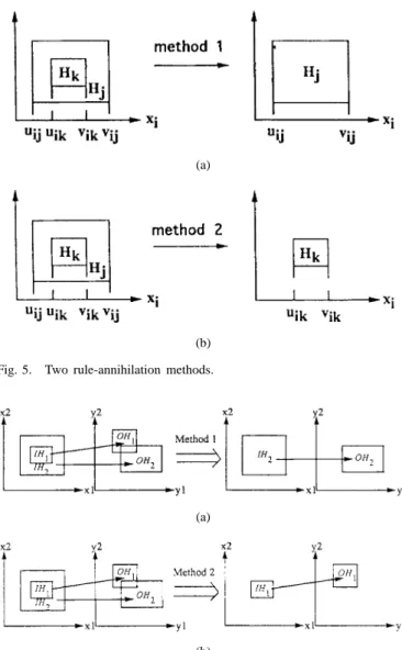
With the above on-line learning algorithm, FALCON-ART, the fuzzy logic rules can only be created and cannot be annihilated. It would be better if the FALCON-ART has the ability to delete unnecessary or redundant rules. In this section, we shall present two methods of rule annihilation. The basic idea is to combine two or more “similar” rules into a representative one. During the on-line structure/parameter learning, the hyperboxes of input and output spaces are tuned. These hyperboxes may be updated to greater hyperboxes or smaller hyperboxes gradually. Thus, the perfect inclusion between two hyperboxes may happen. Let’s consider the situation that the hyperbox contains the hyperbox ; i.e., the hyperbox is a subset of the hyperbox . In this situation, it is intuitive that one of the hyperboxes ( or ) can be annihilated. This is equivalent to the case that two fuzzy terms of a linguistic variable represent redundant fuzzy meaning and thus one of them can be removed.
To determine the rule similarity, a dimension-by-dimension comparison process of hyperboxes is conducted. Let
and be the edges of two compared hyperboxes
and in the th dimension. If and for
all dimensions , in the input space or output space we say the hyperbox contains the hyperbox . For such two hyperboxes and , if we annihilate the hyperbox and remain the hyperbox we will obtain the greater hyperbox. This will cause the membership functions to do coarse clustering in the input or output space. On the contrary, if the hyperbox is annihilated and the hyperbox remains, we will obtain the smaller hyperbox and the membership functions will do finer clustering in the input or output space. In the latter case, the training patterns outside the hyperbox will be reclustered in the next iteration. When we decide to annihilate an input hyperbox, we delete all the nodes and attached connections that constitute this hyperbox. We also need to annihilate the output hyperbox associated by this input hyperbox if this output byperbox is not associated by other input byperboxes. On the other hand, if we decide to annihilate a output byperbox, we delete all the nodes that constitute this hyperbox, and then redirect all its input links to the remaining similar output hyperbox. The proposed rule annihilation process is based on the natural property of most control systems that if two input data are close (similar) in the input space, the two mapped outputs are also close (similar) in the output space. Based on the above discussion, we propose two methods to determine the combination of two similar rules. The first method is to keep the greater hyperbox in the input and output spaces, whereas the second method is to keep the smaller hyperbox in the input and output spaces. These two methods are described as follows. The rule annihilation process is illustrated in Figs. 5 and 6, where we consider two-input and two-output case.
(a)
(b) Fig. 5. Two rule-annihilation methods.
(a)
(b)
Fig. 6. Illustrations of the rule-annihilation process in the FALCON-ART model.
1) Method 1: If one hyperbox contains another hyperbox
(i.e., or ), we can delete the
smaller hyperbox (i.e., or ) and keep the greater hyperbox (i.e., or ). This is achieved by letting the left-flat points and perform the fuzzy AND operation for all dimensions and the right-flat points ( and
) perform the fuzzy OR operation for all dimensions
(40)
(41) From these operations we can obtain the greater hyperbox in the input and output spaces [Fig. 5(a)].
The rule-annihilation process in the FALCON-ART is il-lustrated in Fig. 6, which shows a graphic interpretation of Methods 1 and 2 of the rule-annihilation process. Here, we consider a two-input and two-output case. As shown in the figure, two hyperboxes ( ) are formed in the input space and two hyperboxes ( ) are formed in the
output space. The two fuzzy rules indicated in the figure are
“IF is THEN is (Rule 1),” and “IF is
THEN is (Rule 2),” where and
. These rules reflect the natural property of most control problems that if two input data are close (similar) in the input space, the two mapped outputs are also close in the output space. In Fig. 6(a), the hyperbox contains the other hyperbox . According to the Method 1 of rule-annihilation process, we delete the smaller hyperbox and keep the greater hyperbox ; that is, we combine Rules 1 and 2 into Rule 2 as shown in Fig. 6(a).
2) Method 2: If one hyperbox contains another hyperbox
(i.e., or ), we can delete the greater
hyperbox (i.e., or ) and keep the smaller hyperbox (i.e., or ). This is achieved by letting the left-flat points and perform the fuzzy OR operation for all dimensions and the right-flat points ( and ) perform the fuzzy AND operation for all dimensions
(42)
(43) From these operations we can obtain the smaller hyperbox in the input and output spaces [Fig. 5(b)].
We also use Fig. 6 as an example to explain the Method 2 of rule-annihilation process. In Fig. 6(b), the hyperbox contains the other hyperbox . According to Method 2 of rule-annihilation process, we delete the greater hyperbox and keep the smaller hyperbox ; that is, we combine Rules 1 and 2 into Rule 1, as shown in Fig. 6(b).
V. ILLUSTRATIVE EXAMPLES
A general purpose simulator for the FALCON-ART model has been written in “C” language and runs on a PC-486. Using this simulator, four typical examples are presented in this section to show the fundamental applications of the proposed model. The first example is to identify a dynamic system [25], the second example is to predict time-series [17], the third example is to control the truck backer-upper [26], [27], and the fourth example is to control the ball and beam system [16], [28].
Example 1—Identification of the Dynamic System: In this
ex-ample, the proposed FALCON-ART model is used to identify a dynamic system. The identification model has the form
(44) Since both the unknown plant and the FALCON-ART model are driven by the same input, the FALCON-ART model adjusts itself with the goal of causing the output of the identification model to match that of the unknown plant. Upon convergence, the input/output response relationship should match.
The plant to be identified is guided by the difference equation
(45) The output of the plant depends nonlinearly on both its past output values and the input values, but the effects of the input and output values are additive. In applying the FALCON-ART model to this identification problem, the learning rate , sensitivity parameter , and vigilance
pa-rameter , are chosen, where
and are vigilance parameters used in the input and output fuzzy clustering processes, respectively. The training input patterns are generated with
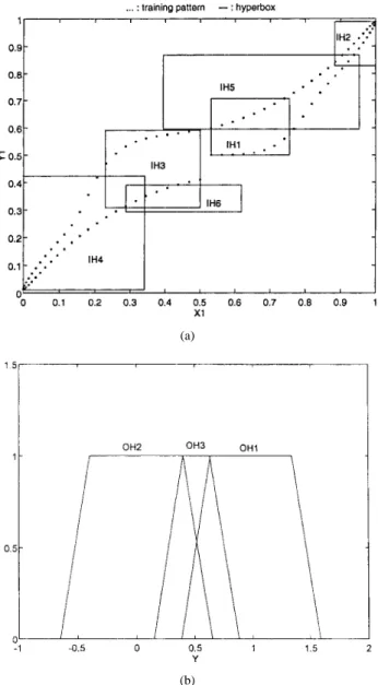
and the training process is continued for 60 000 time steps. Starting at zero, the number of clusters grow dynamically for incoming training data. Each cluster corresponds to a hyperbox in the input or output space. Fig. 7 shows the root-mean-square (rms) errors during learning. Each point on the curve is the average of 200 training time steps. The curve appears to have a big oscillation at the beginning of learning. This situation reflects the structure changing in the early stage of learning; that is, the numbers of fuzzy partitions of and are increasing and new fuzzy logic rules are generated. In this example, the case of two input and one output is considered for illustration. Fig. 8(a) illustrates the distribution of the training patterns and the final assignment of the rules (i.e., distribution of the membership functions) in plain (input space). There are six hyperboxes formed in the input space. Fig. 8(b) shows the distribution of the output membership functions in domain (output space). Three trapezoidal
membership functions are generated in
the output space. After the hyperboxes in the input and output spaces are tuned or created in the fuzzy clustering process, the mapping process then decides proper mapping between the input clusters and output clusters. There are six fuzzy logic rules formed, finally, as in the following:
Rule 1: IF is THEN is Rule 2: IF is THEN is Rule 3: IF is THEN is Rule 4: IF is THEN is Rule 5: IF is THEN is Rule 6: IF is THEN is
where and . From these fuzzy
logic rules, we know Rules 1 and 3 have the same consequent. Also, Rules 2 and 5 and Rules 4 and 6 map to the same consequent. These rules reflect the natural property that if two input data are close (similar) in the input space, the two mapped outputs are also close in the output space. Fig. 9 shows the outputs of the plant and the identification model. In this figure, the output of the FALCON-ART model are presented as dotted curve while plant output values are represented as solid curve. The results show the perfect identification capability of the trained FALCON-ART model.
Fig. 7. Learning curve of the FALCON-ART identifier in Example 1.
(a)
(b)
Fig. 8. Simulation results of the FALCON-ART model without rule annihi-lation in Example 1. (a) The input training patterns and the final assignment of rules. (b) The distribution of output membership functions.
Fig. 9. The outputs of the plant and the identification model.
During the simulation, we also applied the rule-annihilation techniques into the FALCON-ART. The learning results of the FALCON-ART with the Method 1 of rule annihilation are shown in Fig. 10. There are four fuzzy logic rules generated in this case. Fig. 10(a) and (b) show the distribution of the input and output membership functions, respectively. The four generated fuzzy logic rules are “IF is THEN is ,”
“IF is THEN is ,” “IF is THEN is
,” and “IF is THEN is .” If we use Method 2 of rule annihilation, there are five fuzzy logic rules generated when learning is terminated. Fig. 11(a) and (b) shows the distribution of the input and output membership functions in this case. The five generated fuzzy logic rules connecting these two figures are “IF is THEN is ,” “IF is
THEN is ,” “IF is THEN is ,” “IF is
THEN is ,” and “IF is THEN is .”
Simulation results show that with rule-annihilation techniques, we can still obtain perfect identification capability by using fewer fuzzy logic rules.
Notice that the possibility of the occurrence of the perfect inclusion between two hyperboxes is not low. This is the nature of the fuzzy ART and fuzzy ARTMAP algorithms [22], [23]. Especially, when a large hyperbox formed in the input (output) space, a following input pattern may easily fall into it. If this pattern is not considered to belong to the large hyperbox (e.g., the desired output of this pattern is not in the output hyperbox that the large input hyperbox associates with), it will form a new small hyperbox in the large hyperbox and perfect inclusion occurs. Moreover, since our model uses the fast-learn fuzzy ART to decide the initial hyperboxes (structure learning) and the backpropagation algorithm to tune the hyperboxes (parameter learning), a hyperbox may be tuned to include or be included by another hyperbox gradually in the parameter learning step and perfect inclusion between two hyperboxes may happen.
Example 2—Prediction of the Chaotic Time-Series: Let
be a time series. The problem of time-series prediction can be formulated as: given
determine , where
(a)
(b)
Fig. 10. Simulation results of the FALCON-ART model with Method 1 of rule annihilation in Example 1. (a) The input training patterns and the final assignment of rules. (b) The distribution of output membership functions.
to ).
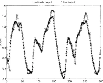
To illustrate the on-line learning ability, the FALCON-ART model is used to predict the Mackey–Glass chaotic time-series. The Mackey–Glass chaotic time-series is generated from the following delay differential equation:
(46) where . In our simulation, we choose the series with . Fig. 12 shows 1000 points of this chaotic series used to test the FALCON-ART model. We choose and in our simulation (i.e., nine point values in the series are used to predict the value of the next time point). The 200 points of the series from – are used as training data, and the final 300 points from – are used as test data. The learning rate , sensitivity parameter
, and vigilance parameter , are
chosen, where and are vigilance parameters used in the input and output fuzzy clustering processes, respectively.
(a)
(b)
Fig. 11. Simulation results of the FALCON-ART model with Method 2 of rule annihilation in Example 1. (a) The input training patterns and the final assignment of rules. (b) The distribution of output membership functions.
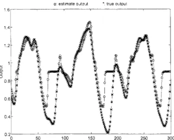
After the structure-parameter learning, there are twenty-two fuzzy logic rules generated in our model. Fig. 13 shows the prediction of the chaotic time series from –
when 200 training data [from – ] are used. In this figure, predictions of the FALCON-ART model are represented as ’s while true values are represented as ’s. The rms error of prediction output approximates 0.08. The results show the good prediction capability of the FALCON-ART model trained only by a small set of training data.
We now compare the performance of our system with that of other existing methods that can generate fuzzy rules from numerical data automatically. The performance indexes considered include numbers of fuzzy rules generated and rms error of prediction output. The comparison results are tabulated in Table I. First, we compare the performance of the FALCON-ART model with that of the system proposed by Wang and Mendel [17]. They developed a general method to generate fuzzy rules from numerical data. This method consists of five steps: Step 1 divides the input and output spaces
TABLE I
PERFORMANCECOMPARISON OFVARIOUSRULEGENERATIONMETHODS ON THETIME-SERIESPREDICTIONPROBLEM
Fig. 12. The Mackey–Glass chaotic time series.
Fig. 13. Simulation results of the time-series prediction from
x(701)–x(1000) using the FALCON-ART model with 22 fuzzy rules
when 200 training data [fromx(501)–x(700)] are used.
of the given numerical data into fuzzy regions by choosing proper membership functions, Step 2 generates fuzzy rules from the given data, Step 3 assigns a degree of each of the generated rules for the purpose of resolving conflicts among the generated rules, Step 4 creates a combined fuzzy rule base based on both the generated rules and linguistic rules of human experts, and Step 5 determines a mapping from input space to output space based on the combined fuzzy rule base using a
Fig. 14. The membership functions used in Wang and Mendel’s system for the chaotic time-series prediction.
defuzzifying procedure. They also chose and in their simulation, i.e., nine point values in the series were used to predict the value of the next time point. The membership functions used in the system are shown in Fig. 14. The 200 points of the series in Fig. 12 from – are used as training data and the final 300 points from – are used as test data. After performing the five steps described in the above, we have 121 generated fuzzy rules. Fig. 15 shows the prediction of the chaotic time series from –
when 200 training data [from – ] are used. The rms error of prediction output approximates 0.08. The results show that the proposed FALCON-ART predictor is able to keep similar rms error but needs fewer fuzzy rules than Wang and Mendel’s system. These results are shown in the second column of Table I.
The second rule-generation method for comparison is called the data-distribution method. This method generates fuzzy rules according to the training data distribution in the in-put/output product space. This method consists of five steps: Step 1 divides the input/output product space of the given numerical data into crisp regions, Step 2 generates fuzzy rules from numerical data allocated in the regions and then decides the weight of each rule according to the number of numerical data falling into each region, Step 3 fuzzifies these crisp regions into fuzzy regions by defining proper membership functions, Step 4 creates a combined fuzzy rule base based on the generated rules, and Step 5 determines a mapping from input space to output space based on the combined fuzzy rule base using a defuzzifying procedure. The membership functions shown in Fig. 14 are also used in the data distribution method for chaotic time series prediction. After performing the five steps stated in the above, we have 118 generated fuzzy rules. Fig. 16 shows the prediction of the chaotic time
Fig. 15. Simulation results of the time series prediction from
x(701)–x(1000) using the Wang and Mendel’s system when 200
training data [fromx(501)–x(700)] are used.
Fig. 16. Simulation results of the time series prediction from
x(701)–x(1000) using the data distribution method when 200 training data
[fromx(501)–x(700)] are used.
series from – when 200 training data are used. The rms error of prediction output approximates 0.08. These results are shown in the third column of Table I. According to these results, the number of fuzzy rules generated in our FALCON-ART model is still much smaller than that of the data distribution method. It is noted that the number of the generated fuzzy rules in the data distribution method and Wang and Mendel’s system cannot be determined by the users. That is, the number of fuzzy rule generated from the data distribution method and Wang and Mendel’s system depends on incoming training patterns.
Kosko [14] proposed the product space-clustering technique to the adaptive fuzzy associative memory (FAM) systems such that they can generate FAM rules directly from training data. The basic concept of automatic generation of FAM rules is to use the adaptive vector quantization (AVQ) algorithm to find and allocate synaptic quantization vectors to FAM cell from input/output training data, and then decide the weight
Fig. 17. Simulation results of the time series prediction from
x(701)–x(1000) using the UCL–AVQ algorithm with 100 fuzzy rules
when 200 training data [fromx(501)–x(700)] are used.
of each FAM cell (FAM rule) according to the number of quantization vectors falling into it. Consider the case that and . The system samples the nonfuzzy input
and output stream . Competitive AVQ
algorithm, which includes unsupervised competitive learning (UCL) and differential competitive learning (DCL), distributes the synaptic quantization vectors to different FAM cells in the space, where is an integer given in advance. To do this, we use a UCL or DCL network with two input nodes and output (competitive) nodes. Assume contains quantization vectors. Then cell counts define a frequency histogram, since all sum to . Hence, weights the corresponding FAM rule. According to the desired number of fuzzy rules or a given rule–weight threshold, a final FAM rule base is generated.
The membership functions in Fig. 14 are also used in the product space-clustering method for the chaotic time-series prediction problem. In our simulation, after competitive AVQ learning we find that the centroid defuzzification process can-not be performed on the used triangular membership functions since some test data do not fire any fuzzy rules in the rule base and thus causes a “divide by zero” problem in the defuzzification process. To solve this problem, we replace triangular membership functions with bell-shaped membership functions. We set the number of rules as 100 and use the fixed weighting of rule calculated from cell count after competitive AVQ learning. Figs. 17 and 18 show the prediction of the chaotic time series from –
using UCL–AVQ and DCL–AVQ algorithms, respectively. The rms errors of prediction output approximate 0.17 and 0.2.
To improve the prediction accuracy, we combine UCL(DCL)–AVQ algorithm with the backpropagation learning algorithm. The former determines the fuzzy rule base and the latter tunes the weighting values of fuzzy rules . For comparison, we consider two cases: and . Figs. 19 and 20 show the prediction of the chaotic time series from – using the UCL-AVQ and backpropagation hybrid learning algorithm. Figs. 21 and
Fig. 18. Simulation results of the time series prediction from
x(701)–x(1000) using the DCL–AVQ algorithm with 100 fuzzy rules
when 200 training data [fromx(501)–x(700)] are used.
Fig. 19. Simulation results of the time-series prediction from
x(701)–x(1000) using the UCL–AVQ and backpropagation hybrid
learning algorithm with 22 fuzzy rules when 200 training data [from
x(501)–x(700)] are used.
22 show the prediction of the chaotic time series from – using the DCL–AVQ and backpropagation hybrid learning algorithm. The results show that the predictor that uses hybrid learning algorithm is able to keep smaller rms error than the original predictor. These results are shown in Table I.
As shown in Table I, the proposed FALCON-ART predictor produces smaller or similar rms error by using fewer fuzzy rules than other rule generation methods. However, these simulation results do not show the perfect prediction capability of the proposed model trained only by a small set of training data. It seems that 200 training data are not enough for the chaotic time-series prediction problem. Thus, we replace 200 training data with 700 training data to train the FALCON-ART predictor. The learning parameters used are the same as those used previously. After the structure-parameter learning, there are 30 fuzzy rules generated and the rms error of prediction
Fig. 20. Simulation results of the time-series prediction from
x(701)–x(1000) using the UCL–AVQ and backpropagation hybrid
learning algorithm with 100 fuzzy rules when 200 training data [from
x(501)–x(700)] are used.
Fig. 21. Simulation results of the time-series prediction from
x(701)–x(1000) using the DCL–AVQ and backpropagation hybrid
learning algorithm with 22 fuzzy rules when 200 training data [from
x(501)–x(700)] are used.
output approximates 0.04. Fig. 23 shows the prediction of the chaotic time series from – when 700 training data [from – ] are used. The simulation results show the perfect prediction capability of the well-trained FALCON-ART. It is noted that the big increase of training data does not induce impractical increase of fuzzy rules in the FALCON-ART model. In [17], Wang and Mendel tried to improve the prediction accuracy by increasing the training data, using the updating fuzzy rule base procedure and dividing the “domain interval” into finer regions in their system. Finally, their system achieved perfect prediction capability when the domain interval was divided into 29 regions. Hence, the price paid for achieving high-prediction accuracy is a larger fuzzy rule base. Recently, Jang [9] proposed a model, called adaptive-network-based fuzzy inference system (ANFIS) architecture, for learning and tuning a fuzzy predictor. By using a hybrid
Fig. 22. Simulation results of the time-series prediction from
x(701)–x(1000) using the DCL–AVQ and backpropagation hybrid
learning algorithm with 100 fuzzy rules when 200 training data [from
x(501)–x(700)] are used.
Fig. 23. Simulation results of the time-series prediction from
x(701)–x(1000) using the FALCON-ART model with 30 fuzzy rules
when 700 training data [fromx(1)–x(700)] are used.
learning procedure, the proposed ANFIS can construct an input/output mapping based on both human knowledge (in the form of fuzzy IF–THEN rule) and stipulated input/output data pairs. The ANFIS also has perfect prediction capability on the chaotic time series prediction problem after learning. However, a set of correct fuzzy logic rules and proper input/output space partition must be given in advance by experts before initiating the training of the ANFIS.
Example 3—Control for Backing Up the Truck: Backing a
truck to a loading dock is a difficult exercise. It is a non-linear control problem for which no traditional control design methods exits. Nguyen and Widrow [26] developed a neural network controller which only used numerical data for the backing up the truck problem. Kong and Kosko [27] proposed a fuzzy controller which only used linguistic rules for the same problem. In this example, we develop a controller (called FALCON-ART controller) to back up a simulated truck to a
Fig. 24. Diagram of the simulated truck and loading zone.
loading dock in a planar parking lot. We use on-line structure-parameter learning algorithm for the FALCON to adaptively generate fuzzy rules and adjust parameters according to train-ing data. This FALCON-ART controller enables the truck to reach the desired position successfully.
The simulated truck and loading zone are shown in Fig. 24. The truck position is exactly determined by three state vari-ables , , and , where is the angle of truck with the horizontal and the coordinate pair specifies the position of the rear center of the truck in the plane. The steering angle of the truck is the controlled variable. The positive values of represent clockwise rotations of the steering wheel and negative values represent counterclockwise rotations. The truck is placed at some initial position and is backed up while being steered by the controller. The objective of this control problem is to use backward movements of the truck only to make the truck arrive at the loading dock at right angle and to have the position of the truck with the desired loading dock . The truck moves backward by fixed distance of the movement of the steering wheel at every step. The loading region is limited to the plane [0, 100] [0, 100].
The input and output variables of the FALCON-ART con-troller must be specified. The concon-troller has two inputs, truck angle and the cross position . Assuming enough clearance between the truck and the loading dock, the coordinate is not considered as an input variable. The output of controller is the steering angle . The ranges of the variables and
are as follows:
(47) (48) (49) The equations of backward motion of the truck are given by
(50) where is the length of the truck. Equation (50) is used to obtain the next state when the present state is given.
For the purpose of training the FALCON-ART controller, learning takes place during several different tries, each starting from an initial state and terminating when the desired state
Fig. 25. The moving trajectories of the truck where the solid curves represent the six sets of training trajectories and the dashed curves represent the moving trajectories of the truck under the control of the learned FALCON-ART controller.
Fig. 26. Learning curve of the FALCON-ART controller in Example 3.
is reached. In our simulation, six different initial positions of the truck are chosen. The six training paths are shown in Fig. 25. The truck moves by a small fixed distance at every step and the length of the truck is set to be . The learning rate , sensitivity parameter , and initial vigilance parameter ,
are chosen. The vigilance values decrease gradually with training epoch number increasing. The training process is continued for 600 epochs. In each epoch, all the six sets of training trajectories are presented once to the FALCON-ART controller in a random order. Fig. 26 shows the learning curves for the FALCON-ART controller. After the on-line structure-parameter learning, there are 19 fuzzy logic rules generated in our simulation. The rms error of the controller with nineteen rules approximates to 2.3 . The training result is shown in Fig. 25. In the figure, the solid curves are the training paths and the dotted curves are the paths that the truck runs under the control of the learned controller. As this figure shows, the FALCON-ART controller can smooth the
Fig. 27. Three-dimensional (3-D) control surface of the learned FAL-CON-ART controller in Example 3.
training paths. The three-dimensional (3-D) control surface of the learned FALCON-ART controller in Fig. 27 shows the steering signal outputs with respect to all the combinations of the two input variable values and after learning the six sets of training trajectories. After the training process is terminated, Fig. 28(a)–(c) shows the trajectories of the moving truck controlled by the FALCON-ART controller starting
from the initial positions (a) ,
(b) , and (c) . If we remove
the truck training trajectories 3 and 4 from the six sets of training trajectories, we find that the learned FALCON-ART controller can still move the truck nearly to the correct parking position starting at the same initial positions. The trajectory
starting at in this case is shown in
Fig. 29. Although we reduce the number of training patterns, this controller can still move the truck to the correct parking position. This indicates that the FALCON-ART controller can also produce appropriate control action even if training patterns are not distributed over a sufficiently varied area in the state space. Therefore, the FALCON-ART has good generalization capability and robustness.
In the case that six sets of training patterns are used during learning process, we also tried the rule-annihilation technique to combine some similar rules. With this learning, there are twelve fuzzy rules generated in the use of Method 1 of rule annihilation and seven fuzzy logic rules generated in the use of Method 2. The results show that by incorporating the rule-annihilation process into the FALCON-ART, we can obtain fewer fuzzy logic rules that can still move the truck to the correct parking position.
Example 4—Control of the Ball and Beam System: The ball
and beam system is shown in Fig. 30. The beam is made to rotate in a vertical plane by applying a torque at the center of rotation; the ball is free to roll along the beam. We require that the ball remain in contact with the beam. The system can be written in the following state-space form:
(51)
(a) (b)
(c)
Fig. 28. Truck moving trajectories starting at three different initial positions under the control of the FALCON-ART model after learning six sets of training trajectories.
where is the state of
the system and is the output of the system. The control is the angular acceleration and the parameters and are chosen in this system. The purpose of control is to determine such that the closed-loop system output will converge to zero from different initial conditions.
According to the input/output-linearization algorithm [28], the control law is determined as follows: for state ,
compute ,
where , , ,
, and the are chosen so that is a Hurwitz polynomial.
Compute and ;
then .
In our simulation, we solve the differential equations using the second/third-order Runge–Kutta method. We train the FALCON-ART model to approximate the aforementioned conventional controller of a ball and beam system. Let all closed-loop poles be placed at . Thus, ,
Fig. 29. Truck moving trajectory under the control the FALCON-ART model after learning four sets of training trajectories.
, , and are chosen. We use
Fig. 30. The ball and beam system.
Fig. 31. The responses of the closed-loop ball and beam system controlled by the FALCON-ART model for four initial conditions.
training pair with obtained from randomly sampling 300
points in the region .
The learning rate , sensitivity parameter ,
and vigilance parameter , are
chosen. After the on-line structure-parameter learning, there are 28 fuzzy logic rules generated in our simulation. We have tested the learned controller at four initial conditions:
, ,
, and .
Fig. 31 shows the output responses of the closed-loop ball and beam system controlled by the FALCON-ART model. These responses approximate those of the original controller for the four initial conditions. As a comparison, Fig. 32 shows the output responses of the closed-loop ball and beam system controlled by the input/output-linearization algorithm for four initial conditions. We also show the behavior of the four states of the ball and beam system starting at the initial condition in Fig. 33. In this figure, the four states of the system decay to zero gradually. The results show the perfect control capability of the trained FALCON-ART model.
VI. DISCUSSION
In this section, we summarize the features of the proposed FALCON-ART model. First, distributed representation is used to represent the input patterns in the FALCON-ART model. This is achieved by the fuzzification process through the adaptive input membership functions. With the adaptive input membership functions, the input space is divided into overlap-ping smaller regions and, more importantly, this partitioning is
Fig. 32. The responses of the closed-loop ball and beam system controlled by the input/output-linearization algorithm for four initial conditions.
Fig. 33. The responses of the four states of the ball and beam system under the control of the learned FALCON-ART controller.
not performed in advance, but is dynamically and appropriately adjusted during the learning process. As a result, each region varies in size and the degree of overlapping between regions is also adjustable. This is in contrast to the Wang and Mendel’s system [17], ANFIS system [9], and Kosko’s system [14] in which the input space need to be divided properly in advance. The second feature of the proposed FALCON-ART model is its dynamic structure-parameter-learning ability that can find proper fuzzy logic rules. This is in contrast to the approaches in [9] and [18], which need a priori control knowledge from expert operators in term of fuzzy control rules. The third feature of the proposed FALCON-ART model is its rule-annihilation ability. The FALCON-ART model has the ability to delete unnecessary or redundant rules. In other words, it can combine some nodes with the same or a very similar control action. The fourth feature of the proposed FALCON-ART model is the ease with which expert knowledge can be incorporated into the network greatly shortening learning time. The fifth feature of the proposed FALCON-ART model is that
it flexibly partitions the input/output spaces according to the distribution of environment states. This avoids the combinato-rial growth problem encountered by partitioned grids in some complex systems. In addition to the simulations done in this paper, the proposed supervised structure-parameter-learning algorithm has been used to solve many practical problems, including crane-position control and adaptive control of elec-trodischarge machining (EDM) in our laboratory.
VII. CONCLUSION
In this paper, we introduced a general connectionist model of a fuzzy logic control system called FALCON. An on-line structure-parameter learning algorithm called FALCON-ART was proposed for constructing the FALCON dynamically. The proposed learning algorithms is able to partition the input and output spaces and then find proper fuzzy rules and optimal membership functions dynamically. The FALCON-ART partitions the pattern space into irregular hyperboxes and, thus, can avoid the problem of combinatorial growing of partitioned grids in some complex systems. Simulations demonstrate that the proposed FALCON-ART model is quite effective in many applications.
REFERENCES
[1] R. R. Yager, “Implementing fuzzy logic controller using a neural network,” Fuzzy Sets Syst., vol. 48, pp. 53–64, 1992.
[2] P. J. Werbos, “Neural control and fuzzy logic: Connections and designs,”
Int. J. Approx. Reasoning, vol. 6, pp. 185–219, 1992.
[3] T. Tagaki and I. Hayashi, “NN-driven fuzzy reasoning,” Int. J. .Approx.
Reasoning, vol. 5, pp. 191–212, 1991.
[4] H. R. Berenji, “An architecture for designing fuzzy controllers using neural networks,” Int. J. Approx. Reasoning, vol. 6, pp. 267–292, 1991. [5] H. Nomura, I. Hayashi, and N. Wakami, “A learning method of fuzzy inference rules descent method,” in Proc. IEEE Int. Conf. Neural
Networks, Baltimore, MD, June 1992, pp. 203–210.
[6] D. Nauck and R. Kruse, “A fuzzy neural network learning fuzzy control rules and membership functions by fuzzy error backpropagation,” in
Proc. IEEE Int. Conf. Neural Networks, San Francisco, CA, Mar. 1993,
pp. 1022–1027.
[7] C. T. Sun and J. S. Jang, “A neuro-fuzzy classifier and its applications,” in Proc. IEEE Int. Conf. Fuzzy Syst., San Francisco, CA, Mar. 1993, pp. 94–98.
[8] J. S. Jang, “Self-learning fuzzy controllers based on temporal back propagation,” IEEE Trans. Neural Networks, vol. 3, pp. 723–741, May 1992.
[9] , “ANFIS: Adaptive-network-based fuzzy inference system,”
IEEE Trans. Syst., Man, Cybern., vol. 23, no. 3, pp. 665–685, May/June
1993.
[10] H. Bersini, J. P. Nordvik, and A. Bonarini, “A simple direct adaptive fuzzy controller derived from its neural equivalent,” in Proc. IEEE Int.
Conf. Neural Networks, San Francisco, CA, Mar. 1993, pp. 345–350.
[11] I. Enbutsu, K. Baba, and N. Hara, “Fuzzy rule extraction from a multilayered neural network,” in Proc. IEEE Int. Joint Conf. Neural
Networks, Seattle, WA, July 1991, pp. 461–465.
[12] C. C. Lee and H. R. Berenji, “An intelligent controller based on approximate reasoning and reinforcement learning,” in Proc. IEEE Intell.
Mach., Albany, NY, Sept. 1989, pp. 200–205.
[13] E. Khan and P. Venkatapuram, “Neufuz: Neural network based fuzzy logic design algorithms,” in Proc. IEEE Int. Conf. Fuzzy Syst., San Francisco, CA, Mar. 1993, pp. 647–654.
[14] B. Kosko, Neural Networks and Fuzzy Systems. Englewood Cliffs, NJ: Prentice-Hall, 1992.
[15] L. X. Wang and J. M. Mendel, “Backpropagation fuzzy rules as nonlinear dynamic system identifiers,” in Proc. IEEE Int. Conf. Fuzzy
Syst., San Diego, CA, Mar. 1992, pp. 1409–1418.
[16] , “Fuzzy basis functions, universal approximation, and orthogo-nal least-squares learning,” IEEE Trans. Neural Networks, vol. 3, pp. 807–814, May 1992.
[17] , “Generating fuzzy rules by learning from examples,” IEEE
Trans. Syst., Man, Cybern., vol. 22, no. 6, pp. 1414–1427, Nov./Dec.
1992.
[18] H. R. Berenji and P. Khedkar, “Learning and tuning fuzzy logic controllers through reinforcements,” IEEE Trans. Neural Networks, vol. 3, pp. 724–740, May 1992.
[19] C. T. Lin and C. S. G. Lee, “Neural-network-based fuzzy logic control and decision system,” IEEE Trans. Comput., vol. 40, pp. 1320–1336, Dec. 1991.
[20] , “Real-time supervised structure/parameter learning for fuzzy neural network,” in IEEE Int. Conf. Fuzzy Syst., San Diego, CA, Mar. 1992, pp. 1283–1290.
[21] , “Reinforcement structure/parameter learning for an integrated fuzzy neural network,” IEEE Trans. Fuzzy Syst., vol. 2, pp. 46–63, Feb. 1994.
[22] G. A. Carpenter, S. Grossberg, and D. B. Rosen, “Fuzzy ART: Fast stable learning and categorization of analog patterns by an adaptive resonance system,” Neural Networks, vol. 4, pp. 759–771, 1991. [23] G. A. Carpenter, S. Grossberg, N. Markuzon, J. H. Reynolds, and D. B.
Rosen, “Fuzzy ARTMAP: A neural network architecture for incremental supervised learning of analog multidimensional maps,” IEEE Trans.
Neural Networks, vol. 3, pp. 698–712, May 1992.
[24] P. K. Simpson, “Fuzzy min-max neural networks—Part 2: Clustering,”
IEEE Trans. Fuzzy Syst., vol. 1, pp. 32–45, Feb. 1993.
[25] K. S. Narendra and K. Parthasarathy, “Identification and control of dy-namical systems using neural networks,” IEEE Trans. Neural Networks, vol. 1, pp. 4–26, Jan. 1990.
[26] D. Nguyen and B. Widrow, “The truck backer-upper: An example of self-learning in neural network,” IEEE Contr. Syst. Mag., vol. 10, no. 3, pp. 18–23, Apr. 1990.
[27] S. G. Kong and B. Kosko, “Comparison of fuzzy and neural truck backer-upper control systems,” in Int. Joint Conf. Neural Network, San Diego, CA, June 1990, vol. 3, pp. 349–358.
[28] J. Hauser, S. Sastry, and P. Kokotovic, “Nonlinear control via approx-imate input–output linearization: The ball and beam example,” IEEE
Trans. Automat. Contr., vol. 37, no. 3, pp. 392–398, Mar. 1992.
Cheng-Jian Lin (S’94–M’95) received the B.S. degree in electrical engineering from Tatung Insti-tute of Technology, Taiwan, R.O.C., in 1986, and the M.S. and Ph.D. degrees in control engineering from the National Chiao-Tung University, Taiwan, R.O.C., in 1991 and 1996, respectively.
Currently, he is an Associate Professor in the Department of Electronic Engineering of Nankai College of Technology and Commerce, Nantou, R.O.C. His current research interests are neural net-works, learning systems, fuzzy control, approximate reasoning, signal processing, and image processing.
Dr. Lin is a member of the IEEE Control Systems Society and the IEEE Systems, Man, and Cybernetics Society.
Chin-Teng Lin received the B.S. degree in control engineering from the National Chiao-Tung Univer-sity, Taiwan, R.O.C., in 1986, and the M.S.E.E. and Ph.D. degrees in electrical engineering from Purdue University, West Lafayette, IN, in 1989 and 1992, respectively.
Since August 1992, he has been with the College of Electrical Engineering and Computer Science, National Chiao-Tung University, Hsinchu, Taiwan, R.O.C., where he is currently a Professor of control engineering. He is the co-author of Neural Fuzzy
Systems—A Neuro-Fuzzy Synergism to Intelligent Systems (Englewwod Cliffs,
NJ: Prentice-Hall, 1996) and the author of Neural Fuzzy Control Systems with
Structure and Parameter Learning (River Edge, NJ: World Scientific, 1994).
His current research interests are fuzzy systems, neural networks, intelligent control, human-machine interface, and video and audio processing.
Dr. Lin is a member of Tau Beta Pi and Eta Kappa Nu. He is also a member of the IEEE Computer Society, the IEEE Robotics and Automation Society, and the IEEE Systems, Man, and Cybernetics Society.