國立高雄大學資訊工程學系
碩士論文
對異質性處理器系統上的工作以加權方式作截限時間分配
Weighted Deadline Assignment for Tasks on Heterogeneous
Processor Systems
研究生:海英琪 撰
指導教授:郭錦福
ii
誌謝
經過了這兩年在研究所的洗禮,終於順利地從這個容易進但不容易出的窄門離開 了。其中讓我最感念的就是我的指導教授— 郭錦福老師,他不但每每在我有任何問題的 時候總是熱心地幫助我解決,也十分關心學生的生活。而且老師對待學生都很有耐心, 跟老師相處的時間也十分的融洽。實在很感謝老師一路來給予我的幫助與支持。 此外,我還想謝謝在我身邊幫助我並且與我一起努力的同學。雖然大家不同實驗 室,但是也因為系上每屆只有收十個學生的關係,大家的感情都很好,尤其是坤益與嘉 鈞。 最後我想感謝的是我的家人,雖然在學習過程中家裡發生了一些事情,但是他們仍 然無止盡地付出,好讓我能夠更安心地在學業上努力。感謝你們,我愛你們。iii
對異質性處理器系統上的工作以加權方式作截限時間分配
指導教授:郭錦福 博士 國立高雄大學資訊工程學系 學生:海英琪 國立高雄大學資訊工程學系 摘要 嵌入式多媒體系統在現今變得越來越普及,且其有著需要大量運算能力的需求特 性。因此,單一處理器的架構便不適合應用在這個環境中。而在異質性多處理器的架構 下,其通常由數個通用處理器以及專用處理器所組成,因此能夠提供較大的運算能力給 多媒體軟體。此外,在這個架構下,工作需要在不同的處理元件上執行,因此工作通常 會根據其執行需求被切割成許多子工作,且這些子工作仍然必須要維持原本執行的先後 順序關係。本篇論文著重於如何在異質性多處理器的架構上考量即時工作的排程,並且 針對通用處理器以及專用處理器的特性不同來考量各自適合的可排程測試,以維持即時 系統的限制。在本篇論文中,我們提出了一個基於Earliest-Deadline-First 的即時排程演 算法,並且提出了可排程測試分析用以測試工作是否可以排程。此外,使用者可能會想 讓更多的非週期性工作加入到系統中,因此我們將工作的截限時間以加權方式作調整, 並且整合於Total Bandwidth Server 的概念中,好讓處理器的負載能夠傾斜而不平衡,來 排更多的非週期性工作。而在最後,我們用許多實驗證明了我們的方法能夠得到較好的 效果。iv
Weighted Deadline Assignment for Tasks on
Heterogeneous Processor Systems
Advisor: Dr. Chin-Fu Kuo
Department of Computer Science and Information Engineering National University of Kaohsiung
Student: Ying-Chi Hai
Department of Computer Science and Information Engineering National University of Kaohsiung
ABSTRACT
As we known, the multimedia embedded systems become more and more popular and require powerful computation ability. Uniprocessor architecture is not suitable for the high computation complexity. Heterogeneous multiprocessor architecture has been adopted in many embedded systems, which is usually composed of general purpose processors and specific purpose computing components. In such a system, tasks often need to be processed at multiple different functional processing units. Therefore a task is usually divided into several subtasks according to its execution requirements and the subtasks are executed at particular processing unit with precedence constraints. This thesis focuses the problem of task scheduling on a heterogeneous multiprocessor system which consists of a general purpose CPU and a specific purpose DSP. Within considering the different features between the general purpose processor and specific purpose one, we should adopt distinct and suitable admission control to ensure the real-time guarantees. In this thesis, we present an EDF-based scheduling algorithm and propose the schedulability test analysis. To accept more regular sporadic tasks into the system, a weighted deadline assignment strategy is proposed and we integrate the Total Bandwidth Server that exploit the system computing capacity to deal with sporadic tasks. The capability of the proposed scheme is evaluated by a series of experiments, for which we have encouraging results.
Keywords: Real-time, Scheduling, Heterogeneous, Multiprocessor, Deadline Assignment
Contents
口試委員會審定 i 致謝 ii 中文摘要 iii Abstract iv Contents vList of Figures vii
List of Tables viii
1 Introduction 1 1.1 Research Background . . . 1 1.2 Related Work . . . 2 1.3 Research Motivation . . . 3 2 System Model 6 2.1 Processor Model . . . 6 2.2 Task Model . . . 7
3 Real-Time Task Scheduling on Two Heterogenous Processor Sys-tem 9 3.1 Deadline Assignment for Subtasks on Processors . . . 9
3.2 Online EDF-based Scheduling Algorithm . . . 12
3.3 Off-line Schedulability Test Analysis . . . 14
3.3.2 On the Digital Signal Processor . . . 15
3.4 Weighted Deadline Assignment (WDA) . . . 16
4 Simulation and Performance Evaluations 21 4.1 Experiment Environment Setting . . . 21
4.2 Simulation Result . . . 24
4.2.1 Schedulability Test . . . 24
4.2.2 Integration with Total Bandwidth Server . . . 28 5 Conclusion and Future Work 32
List of Figures
1.1 The upper bound of Rate-Monotonic algorithm . . . 4
2.1 Architecture configuration of the dual-core system . . . 6
2.2 Execution of a DSP task . . . 8
3.1 Illustration of schedulers on dual-core systems . . . 10
3.2 Example of splitting DSP task to subtasks . . . 12
3.3 Tradeoff between the load on the DSP and the GPP with different γ . 16 3.4 Example of the functionality of γ . . . 18
4.1 Performance of different schedulability test methods . . . 25
4.2 Admission control with sporadic task sets, where ki,dsp = ci,dspci . . . . 26
4.3 Application of TBS where the system load is 0.7 . . . 29
4.4 Application of TBS where the system load is 0.3 . . . 29
4.5 Schedulability test under different γ values where Cmax = 1000, Dmin = 10000 and K = 0.1 . . . 31
List of Tables
4.1 Parameters for the extended experiments . . . 23 4.2 Parameters for the Total Bandwidth Server experiments . . . 24
Chapter 1
Introduction
1.1
Research Background
The applications, which need higher computational functionality while meeting the real-time constraints in the embedded system at the same time, encounter much more rigor with the growth of application complexity. As the applications of mul-timedia system likewise, the processor also demands enough power to handle the video or audio streams, such as the decoding or encoding of the high-quality video compression format H.264 [1] or the Advanced Audio Coding (AAC ) [2].
For the higher computational demands of real-time applications, there are two main fashion to achieve the goal. The first fashion is to speed the processor up by means of deeper pipeline and the advance of IC technology. However, tasks are preempted with the asynchronous events to meet the real-time constraints such that the system not only losses the benefits of pipeline but also impacts additional overhead. Moreover, although the processor speed becomes faster with the advance of IC technology, it causes the problems of higher power consumption and thermal discharge too. It is not a trustworthy fashion to some devices which need to limit the power supply. The second fashion is to cope with data simultaneously on the strength of extra processors to support the system more computational capacity. The products of Intelr CoreT M2 duo and Intelr CoreT M2 quad nowadays are on
the basis of this concept. Besides, the uniprocessor architecture development not only suffers the bottleneck of IC processes but has the more cost than multiprocessor architecture. Thereby, the multiprocessor architecture platform becomes more and
more popular to the applications with higher computational capacity for meeting the fast-grown demand of applications and increasing the performance of whole system. Besides, heterogenous multiprocessor platforms has become the major trend. For example, “TMS320DM6446” of Texas Instruments is a powerful embedded system platform to support highly-computing requirement of multimedia applications [3].
The multiprocessor system can be typically classified to two kinds of architec-tures: homogenous and heterogenous. The homogenous multiprocessor system as implied by the name has serval identical processors. On the contrary, the het-erogenous multiprocessor system has different characteristics processors including the general purpose processors (GPP) and the special purpose processors (DSP). Among this two kinds of processors, the DSPs are dedicated to handle the complex large mathematic equations and the decoding or encoding of multimedia streams. Moreover, because the DSPs have large amount of registers to speed the computa-tion up, the operacomputa-tion fashions of them are non-preemptable to avoid the overhead of unnecessary context switch. In opposition to DSPs, due to the GPPs are not ded-icated to special purpose, the frequency of GPPs must be much higher than DSPs to be evenly matched with handling some special applications. Hence the homogenous multiprocessor systems lose their predominance under the consideration of cost. Fur-thermore, the architecture of DSPs is provided with predictable execution time, it has more advantage in real-time system. Consequently, the application of heteroge-nous multiprocess systems become noteworthiness in industry, such as automotive systems, communication network, consumer electronics and mobile handhelds.
1.2
Related Work
Nevertheless, many researchers have made their studies on the scheduling in the homogenous multiprocessor systems: A pioneering ”the highest actual density first (HAD)” algorithm which takes the actual remaining density into account to schedule a set of periodic tasks is presented in [4]. An EDF-based schedulability test and
EDF(k) algorithm with periodic task sets are shown by Goossens et al [5]. Baker
purposes an analysis of schedulability test with the preemptive earliest deadline first algorithm and deadline monotonic algorithm on m identical processors in [6].
Besides, a new schedulability test, dedicated to preemptive deadline scheduling of periodic or sporadic tasks on a single-queue m-server system, is proposed with a new concept, called a µ-busy interval [7].
Those researches mentioned above are preemptive algorithms. On the other hand, some scholars develop their schedulability tests based on non-preemptive al-gorithms, such as: Sanjoy purposes a feasibility analysis based on non-preemptive earliest-deadline first algorithm upon several identical processors in [8]. An on-line non-preemptive scheduling algorithm that is easy to be implemented for both, un-derload and overload upon the homogenous multiprocessor system is investigated in [9].
On the contrary, it is relative to be scanty of researches in heterogenous multipro-cessor systems. One of the most significant reason is that the problems of real-time system are NP-hard [10] and the characteristics of heterogenous multiprocessor sys-tem lead the problems to be more complex. However, our thesis focuses the previous research problem model in heterogenous multiprocessor system [11, 12, 13]. Gai et al, first points out that when the traditional scheduling algorithm such as [13] sched-ules tasks which need to be executed on DSP, a hole within each job is generated in the schedule of the GPP, and then they analyze the scenario when tasks are scheduled via Rate-Monotonic scheduling algorithm (RM) [14] to make more accu-rate the schedulability bound [12]. Due to the system model in [12] has two waiting queues (one for GPP and the other for DSP). When the DSP is active, the scheduler selects tasks from the GPP queue only. Nevertheless, the task which needs to be executed on DSP still should have the right to be executed on GPP when its partial work which needs to be executed on GPP doesn’t finish. Previous problem model is improved in [11].
1.3
Research Motivation
Under traditional real-time applications, the system decides the execution priorities of tasks according to their periods or deadlines. Many researches of real-time sys-tem are on the foundation of this basic phenomenon over the years, such as network, database and disk I/O. Even so, with the growth of complexity of real-time
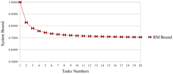
appli-Figure 1.1: The upper bound of Rate-Monotonic algorithm
cations in embedded system, tasks often need to be split to execute on different processor environments, i.e., the heterogenous multiprocessor architecture (GPPs and DSPs), to satisfy the performance and real-time constraints. For instance, a video decode program must decode 30 frames per second. During the digital pro-cessing , GPP reads the data of video from disks in the first stage. The second stage is to call DSP to decode the data and then GPP shows the manipulated data on the monitor in the final stage. However, this action influences the efficiency of traditional real-time scheduling algorithms.
Moreover, most researches assume that task priorities are static in favor of us-ing Rate-Monotonic schedulus-ing algorithm (RM) [14] to simplify the system model. However, As we know the schedulability upper bound of RM scheduling depends on the total number of tasks: n × (21n− 1), where n is the number of tasks. It supports
the highest upper bound 1 while there is only one task in the system but tends to the minimal upper bound 0.69 if n = 10 as the Figure 1.1 shown. Against RM scheduling algorithm, the Earliest-Deadline-First scheduling algorithm (EDF) [14] only takes the total utilization of tasks into account and its upper bound is 1. Even so, it is more difficult to analyze the scenario under EDF scheduling algorithm just because it dynamically assigns task priorities according to their emergency in runtime. As the reason mentioned above, there is seldom research to analyze the phenomenon while assigning task deadlines under different characteristics based on EDF scheduling algorithm.
the DSP queue doesn’t break off when DSP is active against [12]. Furthermore, in order to improve the upper bound limit, we choose Earliest-Deadline-First (EDF) scheduling algorithm as our basis algorithm instead of RM algorithm. Note that the schedulability tests of prior researches just calculate the total utilization of GPP, but we count both the DSP and GPP utilizations separately in our schedulability tests. It give a more precise analysis than previous researches. Finally, we evaluate the effect of the proposed algorithms by a series of simulations. Our thesis proposes the contributions:
• To offer a precise schedulability test analysis for task scheduling in
heteroge-nous multiprocessor systems.
• To propose a weighted deadline assignment strategy to let the system accept
more sporadic tasks.
In Chapter 2, we first introduce the architecture of a heterogenous multipro-cessor system. And we then propose our deadline-assignment method considering that the platform has different processors and tasks have non-preemptive execution requirements on the DSP. We illustrate the simulation and propose the evaluation results in Chapter 4. Finally, Chapter 5 presents an inductive conclusion of this thesis and our future work.
Chapter 2
System Model
2.1
Processor Model
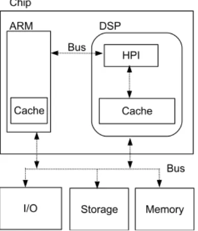
In this section, we will describe the processor architecture in this thesis. The system architecture is composed of two different kinds of computational units named general purpose processor (GPP) and digital signal processor (DSP), respectively, is built in the same chip. Hence, the heterogenous multiprocessor system can exchange message to each other via sharing a common bus. Figure 2.1 illustrates the abstract of heterogenous dual-core architecture.
Figure 2.1: Architecture configuration of the dual-core system
For instance, in the playback upon TMS320C64x of Texas Instruments [3], the general purpose processor (ARM9) saves the captured raw frame data from the video capture device to the common memory shared by the GPP and the DSP, and then invokes the DSP to begin encoding those data using a video encoder algorithm. After above steps, the GPP writes those handled data to the file system.
The functionality of host port interface (HPI) in Figure 2.1 lets the GPP can directly access the cache of the DSP and thereby speed the communication up. Furthermore, the two processors are built on the same chip and both can share the memory address space of the architecture, we can assume that the communication overheads between the GPP and the DSP can be considered as negligible. Even if some possible communication overheads still exist when tasks invoke requests on the GPP or migrate to another core, we can put it into account in priori. Hence, we can classify the system model as similar as system-on-a-chip (SoC) architecture. Note that the GPP not only communicates with the DSP but also directly controls the other peripherals.
In the system, all the jobs launching on a DSP are invoked by a remote procedure call (RPC) and are executed in a non-preemptive fashion. Such RPC is also called
DSP activity and scheduled by the GPP. Therefore, the GPP has the responsibility
of the real-time kernel to prevent that a task invokes a DSP request when there is at least one task on the DSP.
2.2
Task Model
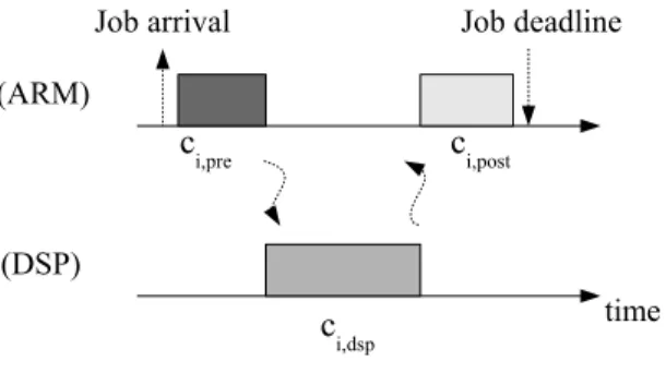
Figure 2.2 illustrates the considered real-time task model on the two heterogeneous processor system. Each task τiis a stream of job instances generated in runtime. For
example, a decoder task needs to decompress about 30 encoded frames per second. The task reads the video file on the GPP, decompress the data on the DSP, and then display the frame on the GPP. For frame encoding, the execution sequence is similar to decoding procedure [15]. Therefore, each job τi,j which arrives at time
ri,j needs ci,gpp = ci,pre+ ci,post unit of time on the GPP. ci,pre and ci,post are for the
data reading and frame displaying, respectively, in a decoder task. The job also need ci,dsp unit of time and on the DSP. Besides, we assume that there is at most
one DSP request invoked by each job during its execution after ci,pre unit of time.
When a job finishes its DSP activity it then executes for ci,post unit of time, so that
ci,pre+ ci,post = ci,gpp.
Definition 1. If a task needs to be executed on the DSP, it is regarded as a DSP
Figure 2.2: Execution of a DSP task
Moreover, jobs should arrive periodically (i.e., ri,j− ri,j−1= Ti, where Ti denotes
the task’s period) or sporadically (that is ri,j−ri,j−1 ≥ Ti, where Ti means minimum
interarrival time) and end before the absolute deadline adi,j. Therefore, the relative
deadline di = adi,j−ri,j. A regular task, in fact, is equal to a DSP task with ci,dsp= 0
but for the sake of simplicity, we disrepute regular tasks as DSP tasks when their
ci,dsp = 0. Finally, ui denotes the utilization of task τi, where
ui =
ci
min(di, Ti)
Chapter 3
Real-Time Task Scheduling on
Two Heterogenous Processor
System
In this chapter, we propose the on-line EDF-based scheduling algorithm and apply the deadline assignments for off-line schedulability test and on-line admission con-trol. To accept more sporadic tasks on the GPP or the DSP separately, we adjust the load of the GPP or the DSP to make the load unbalanced to let more sporadic tasks be accepted. Therefore, the weighted deadline assignment strategy (WDA) which adjusts the relative deadline of subtasks with a weighted parameter γ is proposed.
3.1
Deadline Assignment for Subtasks on
Proces-sors
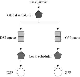
In order to guarantee the real-time requirements of tasks on the system with two heterogenous processors, the idea behind our proposed approach is to assign the relative deadlines to the subtasks of a DSP task and do the off-line schedulability analysis. In runtime, when the processor (i.e., GPP or DSP) is idle, the global scheduler dispatchs the subjob with the most urgent absolute deadline in the corre-sponding ready queues to the processors. As forementioned, the system maintains a global scheduler that has the responsibility to dispatch subjobs to appropriate processors, as Figure 3.1 shown, against local scheduler that only deals with its own
Figure 3.1: Illustration of schedulers on dual-core systems
processor such as GPP or DSP. Furthermore, the scheduling strategy of the sched-uler is EDF [14]. In this section, first we discuss how to assign the relative deadlines to the subtasks of a DSP task.
A DSP task is composed of three subtasks that carry out on different processors according to their execution requirements. Each subtask can be considered as a stream of subjobs. The subtasks of task τi can be viewed as individual and
indepen-dent tasks with equal period but different absolute deadlines. Let di,pre, di,dsp and
di,post represent the relative deadline of three subtasks, i.e., τi,pre, τi,dsp, and τi,post of
task τi, respectively. If a job τi,j arrives at ri,j, its corresponding subjobs are τi,j,pre,
τi,j,dsp, and τi,j,post. Let adi,j,pre, adi,j,dsp, and adi,j,post denote the corresponding
ab-solute deadlines of the subjobs. The abab-solute deadline of subjob τi,j,pre/(τi,j,dsp) is
the ready time of subjob τi,j,dsp/(τi,j,post). The absolute deadlines are derived by the
following equations:
adi,j,pre= ri,j+ di,pre.
adi,j,dsp = adi,j,pre+ di,pre.
adi,j,post= adi,j,dsp+ di,post.
The subjobs τi,j,pre and τi,j,post are then saved in the corresponding ready queue
the subjobs in the queues based on their absolute deadlines.
The relative deadlines of subtasks can be assigned according to different deadline assignment strategies such as Effective Deadline (ED), Equal Slack (EQS), Equal Flexibility (EQF) in [16] and Equal Deadline (EQD). The formulas of the deadline assignment strategies are shown in the following:
Effective Deadline (ED):
di,pre = Ti− (ci,dsp+ ci,post). (3.1a)
di,dsp = Ti− (di,pre+ ci,post). (3.1b)
di,post = Ti− (di,pre+ di,dsp). (3.1c)
Equal Slack (EQS):
di,pre = ci,pre+ Ti− (ci,gpp+ ci,dsp) 3 . (3.2a) di,dsp = ci,dsp+ Ti− (ci,gpp+ ci,dsp) 3 . (3.2b) di,post = ci,post+ Ti− (ci,gpp+ ci,dsp) 3 . (3.2c) Equal Flexibility (EQF):
di,pre = Ti× ( ci,pre ci,gpp+ ci,dsp ). (3.3a) di,dsp= Ti× ( ci,dsp ci,gpp+ ci,dsp ). (3.3b) di,post= Ti× ( ci,post ci,gpp+ ci,dsp ). (3.3c) Equal Deadline (EQD):
di,pre= di,dsp = di,post =
Ti
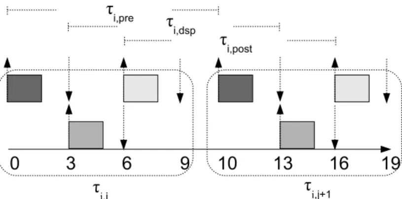
3. (3.4a) For instance, a DSP task τi with di = 9, Ti = 10, ci,pre = ci,dsp = ci,post = 1,
under the deadline assignment strategy EQF. In Figure 3.2, τi,j,pre arrives at time 0,
for the reason that we can visualize the subjob of τi,pre of τi as an independent and
Figure 3.2: Example of splitting DSP task to subtasks
The subjobs of τi,j,dspand τi,j,posthave the properties s similar as τi,j,pre. The period of
the three subtasks are all equal to 10. The most difference is adi,j,dsp = adi,j,pre+dk =
3 + 3 = 6 and adi,j,post = adi,j,dsp+ di,pre = 6 + 3 = 9. Note that The different color
boxes represent the subtasks of the DSP task.
3.2
Online EDF-based Scheduling Algorithm
The proposed Online EDF-based Scheduling Algorithm (OESA) is based on EDF scheduling algorithm [14], that always assigns the highest priority to the job with the absolute deadline nearest to the current time. The most significant difference about the scheduling strategy in this thesis is the scheduler takes no absolute deadlines of jobs but absolute deadlines of subjobs as the foundation of priority assignment in runtime, i.e., the subjob whose absolute deadline is the closest to the current time of all subjobs of all ready jobs has the highest priority to be executed. If a job finishes its partial works on one processor GPP(/DSP)and it still needs to be executed on the other processor DSP(/GPP) whose characteristics is different from the previous one, the job then is migrated to the other processor. Algorithm 1 describes the scheduling situation in detail.
Whenever a scheduling event occurs such as subjob finishes and new job released, etc, the global scheduler is invoked. The scheduler has the two queues, G-queue and D-queue to maintain job information. The elements in the queues are in the order of non-decreasing absolute deadlines. Besides, we use two variables named nowGPP and nowDSP to keep the information of jobs running on the GPP and the DSP, respectively.
Algorithm 1: Online EDF-based Scheduling Algorithm (OESA) /* Deals with the operations while a subjob of job τi,j is
finished or job τi,j arrives */
if subjob of job τi,j finishes then
1
if the status of job τi,j == pre then
2
if ci,dsp != 0 then
3
The status of job τi,j := dsp;
4
Insert nowGPP into D-queue;
5
nowGPP := Null;
6
else
7
if the status of job τi,j == dsp then
8
if ci,post != 0 then
9
The status of job τi,j := post;
10
Insert nowDSP into G-queue;
11
nowDSP := Null;
12
else
13
if the status of job τi,j := post then
14
nowGPP := Null;
15
if job τi,j arrives then
16
Insert job τi,j into G-queue;
17
/* Checking the urgency of jobs */ if the first element of G-queue has a more urgent deadline than the deadline
18
of nowGPP then
Insert nowGPP into G-queue;
19
nowGPP := the first element of G-queue; if nowDSP := Null then
20
nowDSP := the first element of D-queue;
21
Execute the corresponding operation of nowGPP and nowDSP.
From steps 1 to 15, the scheduler deals with the operations after subjobs comple-tion by checking the statuses of jobs, such as changing statuses or clearing nowGPP and nowDSP. There are three kinds of statuses of job named pre, dsp, and post, respectively, and the order of them takes turns. Each status represents the execution requirement of job now. Hence, a job has no status of dsp if it is a instance of a regular task. From steps 16 to 19, the scheduler checks if the subjob of the new arrival job is more urgent than the current running subjob. If the result is true, the running subjob will be preempted. Finally, because of the non-preemptive fashion of DSP, the scheduler must check whether DSP is active or not before assigning subjob to it in step 20.
3.3
Off-line Schedulability Test Analysis
In our study, we propose a off-line schedulability test analysis to determine whether the system with n tasks is schedulable or not, which is divided into two parts. The first part is used for the consideration of the GPP and the other is used for the DSP. As long as one of them is failed, the system is unschedulable.
3.3.1
On the General Purpose Processor
As we mention in Section 3.2, the scheduling algorithm we adopt is on the basis of EDF algorithm. Hence, the utilization upper bound which determines a system is feasible or not is equal to 1. Theorem 1 gives a complete depiction.
Theorem 1. [17] A system of n independent, preemptable tasks is schedulable upon
one processor via the EDF algorithm if the total utilization of the tasks is not more than 1.
Theorem 1 is applied to uniprocessor system without considering the existence of DSP tasks. However, as forementioned visualization, the subtasks of the same task are viewed as individual and independent tasks with equal period but different deadlines. Therefore the utilization ui,pre of subtask τi,pre is equal to min(dci,prei,pre,Ti).
The deriving of ui,dsp and ui,post are similar to ui,pre. Besides, because the relative
ui,preto cdi,prei,pre for subtask τi,pre. Before we extend Theorem 1 to the system we study,
we define some notations first.
• UT is the total utilization of task set T in system.
• Φ is the task set whose subtasks need to execute on DSP in system. • ui,dsp denotes the utilization of τi,dsp, where ui,dsp= uci,dspi,dsp.
• ui,post denotes the utilization of τi,post, where ui,post = dci,posti,post.
Because of the characteristics of splitting jobs, we then conclude the following corollary that deal with the GPP schedulability.
Corollary 1. A system with the task set T , where T consists of n independent and
preemptable tasks, is schedulable via the EDF algorithm if
UT = X τi∈Φ (ui,pre+ ui,post) + X τi∈T −Φ ui ≤ 1. (3.5)
Proof. The proof is a direct consequence of the point of view of visualization
men-tioned behind Theorem 1.
3.3.2
On the Digital Signal Processor
We show the schedulability test on the DSP in this subsection. First, we define some basic notations.
• Cmax is the maximal blocking time of all non-preemptable subtasks on the
DSP, i.e.,
Cmax= max ∀τi∈Φ
{ci,dsp}.
• Dmin is the minimal relative deadline of all non-preemptable subtasks on the
DSP, that is
Dmin = min ∀τi∈Φ
{di,dsp}.
Theorem 2. [18] For a system with non-preemptable subtasks is schedulable via the
EDF algorithm if X τi∈Φ ui,dsp ≤ 1 − Cmax Dmin . (3.6)
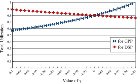
Figure 3.3: Tradeoff between the load on the DSP and the GPP with different γ values
Therefore, we follow Theorem 2 as our scheduling test on DSP. Due to take consideration of different processors, the advantages is not only to enhance the schedulability but to relax the total utilization UT.
3.4
Weighted Deadline Assignment (WDA)
In this section, we further add a weighted parameter γ to adjust the load of GPP and DSP so that to make more bias load balance. Therefore, the system can run more sporadic tasks whose executions are only on the GPP or the DSP. Based on the parameter γ, the new relative deadlines will be derived for computing the total utilization. In this section, we use the parameter γ to adjust the relative deadlines of subtask on the DSP. If the γ value is smaller than 0, it implies that the relative deadline of one subtask on the DSP will be lengthened. Otherwise, it will be shortened.
Figure 3.3 shows that the phenomenon of the tradeoff of load between the GPP and the DSP for a fixed task set under different γ value settings, where the settings of Figure 3.3 are Cmax = 1000, Dmin = 10000 and ci,pre = ci,post = 0.1 × (ci,gpp+ ci,dsp).
For a subtask τi,dsp on the DSP, the decreased relative deadline is added to the
related deadlines of the two subtasks, τi,pre and τi,post, according to the execution
time of the subtask. Besides, from Figure 3.3, we can observe when the γ value becomes smaller, the increased amount of the total utilization of subtasks on the
DSP is smaller than the decreased utilization of subtasks on the GPP.
In this work, we just discuss the situation where the system can schedule more regular tasks (which do not require DSP execution). Therefore, in the following discussion, the γ values are set as negative values. Let ˆdi,dsp denote the newly
derived relative deadline based on the γ value of subtask τi,dsp, where
ˆ
di,dsp= di,dsp× (1 + γ).
For simplicity, in the following sections, we assume that each task in the task set is adjusted by the same γ value.1
The basic deadline assignment strategy we adopt is Equal Flexibility (EQF). However, it it not restricted to use EQF as the based deadline assignment strategy. The designer can choose whatever deadline assignment strategies they want. But from the simulation results in Section 4.2.1 of our study we observe the average per-formance is better while using EQF. The new utilization equations of each subtask can be rewritten as
ˆ
ui,pre =
ci,pre ci,pre×di
ci,pre+ci,dsp+ci,post −
γ×di,dsp×ci,pre ci,pre+ci,post . ˆ ui,post = ci,post ci,post×di
ci,pre+ci,dsp+ci,post −
γ×di,dsp×ci,post ci,pre+ci,post . ˆ ui,dsp = ci,dsp ˆ di,dsp .
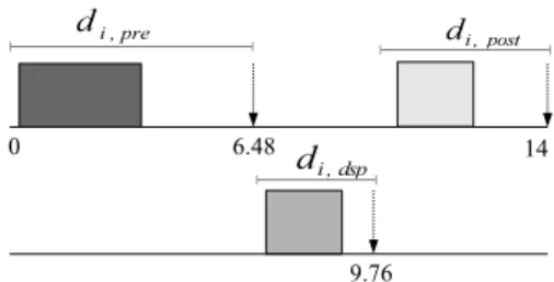
For instance, there is a DSP task τi whose ci,pre = 3, ci,dsp = 2, and ci,post = 2,
and its period is equal to 14. If the γ value is set as −0.18. The relative deadlines allocated to subtasks τi,pre, τi,dsp, and τi,post are from 6, 4 and 4 to 6.48, 3.28 and
4.24, respectively. Figure 3.4 gives above example a clear illustration. ˆ
di,pre and ˆdi,post are contributed by the relative deadline of subtask τi,dsp.
There-fore, the longer relative deadlines τi,pre and τi,post have, the more detriment τi,dsp
1In fact, all tasks are adjusted by γ whether on online or off-line. The scheduler can schedule
tasks with different γ values according to the present system load, and then, the schedulability tests can therefore achieve the upper bounds more closely. However, assigning different γ values to tasks brings out the additional overhead and complicates the algorithm. For simplicity, in our thesis we assume each task has the same γ value.
(a) Initial situation before adjusting with γ
(b) Split of subtasks with γ = −0.18
Figure 3.4: Example of the functionality of γ
suffers. The sum of total utilization of subtasks on GPP and DSP is fixed. It is difficult to estimate that Equation 3.5 or Equation 3.6 has a higher probability of leading scheduling test fail a priori. There is flexibility between the utilizations of subtasks on GPP and DSP. By regulating relative deadlines of the subtasks we want to transfer the failed schedulability test to be successful. To determine the situa-tions, first we make some definitions for convenience beforehand, as showed in the following: ci = ci,gpp+ ci,dsp, ki,pre = ci,preci , ki,dsp= ci,dspci , ki,post = ci,postci , and di ≥ ci.
Note that ki,pre+ ki,dsp+ ki,post = 1.
Based on the definitions, the original relative deadlines of subtasks with EQF are shown as follows:
di,pre = di× ki,pre ≥ ci,pre. (3.7a)
di,post = di× ki,post ≥ ci,post. (3.7b)
di,dsp= di× ki,dsp ≥ ci,dsp. (3.7c)
While considering the parameter γ, the new relative deadlines of subtasks are: ˆ
di,pre = di× ki,pre− di × ki,dsp× γ ×
1
2 ≥ ci,pre. (3.8a) ˆ
di,dsp= di× ki,dsp× (1 + γ) ≥ ci,dsp. (3.8b)
ˆ
di,post= di× ki,post− di× ki,dsp× γ ×
1
Then, the new utilization ˆui,pre of subtask τi,pre is equal to: ˆ ui,pre = ci,pre ˆ di,pre = ci,pre di× ki,pre− di× ki,dsp× γ × 12 . (3.9a) = ci,pre di× (ki,pre− ki,dsp× γ × 12) . (3.9b) = ci× ki,pre di× (ki,pre− ki,dsp× γ × 12) . (3.9c) = ui ki,pre ki,pre− ki,dsp× γ × 12 . (3.9d) and the new utilization ˆui,post of subtask τi,post is equal to:
ˆ ui,post = ci,post ˆ di,post = ci,post di× ki,post− di× ki,dsp× γ × 12 . (3.10a) = ci,post di× (ki,post− ki,dsp× γ × 12) . (3.10b) = ci× ki,post di× (ki,post− ki,dsp× γ × 12) . (3.10c) = ui ki,post ki,post− ki,dsp× γ × 12 . (3.10d) The new utilization ˆui,dsp of subtask τi,dsp is:
ˆ ui,dsp = ci,dsp ˆ di,dsp = ci,dsp di× ki,dsp× (1 + γ) . (3.11a) = ci× ki,dsp di× ki,dsp× (1 + γ) . (3.11b) = ci di× (1 + γ) . (3.11c) = ui 1 1 + γ. (3.11d) Hence, we obtain the new schedulability test equations. There is adjustable flexi-bility to achieve the bias load balance between GPP and DSP if the schedulaflexi-bility test equations below are satisfied, i.e., γ exists.
X τi∈Φ ui( ki,pre ki,pre− ki,dsp× γ × 12 + ki,post ki,post− ki,dsp× γ × 12 ) + X τi∈T −Φ ui ≤ 1. (3.12) X τ∈Φ ui 1 1 + γ ≤ 1 − Cmax Dmin . (3.13)
Note that, when the feasible range of γ is all negative (/positive) except zero, it means the task set, without being adjusted by γ, fails in the schedulability test for the GPP (/DSP). We can let the task set become schedulable with a γ value in the range. Besides, the WDA strategy with γ = 0 is equivalent to EQF strategy.
Chapter 4
Simulation and Performance
Evaluations
The purpose of this chapter is to evaluate the performance of the proposed schedul-ing scheme. We develop a simulation model for the scheme, and use some numerical examples to show the capabilities of our scheme. We investigate two kinds of experi-ments. First we examine the task sets in the heterogenous multiprocessor system to be scheduled or not. Then we apply the WDA strategy to integrate Total Bandwidth Server [19, 20], and evaluate and analyze the phenomenons.
4.1
Experiment Environment Setting
In our experiments, the subtasks on each processor are scheduled via EDF algo-rithm [14]. We design a task generator to produce end-to-end periodic tasks and their workload for each set of the experiments. The performance of our scheduling test analysis is inspected on a large number of task sets by the schedulability test equations (i.e., Equation 3.6 and Equation 3.5), each simulation result is an average over twenty independent simulation runs. The execution times of tasks in a task set are generated by random variables with uniform distribution while the utilization of a task is assigned with poisson distribution. Besides, the experimental environment has the characteristics as follow:
• The total utilization of the system is first randomly generated between 0 and 1,
and then the average utilization of each task is calculated as the seed of poisson distribution. We assign the utilization of each tasks via poisson distribution variable with mean equal to the average utilization of each task.
• In each experimental task set, the proportion of DSP tasks to total tasks is
0.9.
• The ci,pre and ci,post are chosen between 1 to 10 with uniform probabilities, and
the ci,dsp is assigned in the range between 0.5 to 0.8 of ci,gpp.
• The Ti is derived by ci,pre+ci,dspui +ci,post.
At the first experiment, we examine the performance and correctness of our off-line schedulability test. The performance metric is the average schedulability
ratio. The schedulability ratio is the feasible solution number divided by the number
of task sets. We compare the evaluation of three different approaches: MDSS [12],
RSHD [11] and DPCP [13], as description in Section 1.2, against our proposed
method. Moreover, we extend the schedulability test with periodic task sets to adapt to schedule sporadic tasks. That is the schedulability test transforms to
admission control which decides sporadic tasks can be joined to the system or not in
runtime. The parameters settings of the extended experiment are listed as Table 4.1. We set up the minimal interarrival time (MIT ) of sporadic tasks as the same as their period, and the next arrival times (NAT ) of them are chosen evenly between Ti
and 2 × Ti. The attributes of sporadic tasks are somewhat different: each task τi has
density generated by uniform distribution between (0,1], the execution requirement is set between 25 and 50, and each simulation time per tested task set is about three millions unit of time. Besides, we add one additional parameters ρ to denote the proportion of the number of DSP tasks to the number of all tasks in a tested task set. Finally, we compare the four mentioned deadline assignment strategies, i.e., ED, EQS, EQF, and EQD, with ρ = 0.2 or 0.8 and ki,dsp = 0.2 or 0.8.
At the second experiment, we want to extend the WDA deadline assignment strategy to integrate Total Bandwidth Server (TBS) [19, 20]. For simplification, we assume the ki,pre = ki,post = k, so Equation 3.12 and 3.13 in the end of Section 3.4
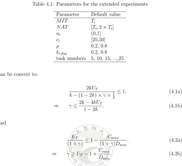
Table 4.1: Parameters for the extended experiments Parameter Default value
MIT Ti NAT [Ti, 2 × Ti] ui (0,1] ci [25,50] ρ 0.2, 0.8 ki,dsp 0.2, 0.8 task numbers 5, 10, 15, ...,25 can be convert to:
2kUT k − (1 − 2k) × γ × 1 2 ≤ 1. (4.1a) ⇒ γ ≤ 2k − 4kUT 1 − 2k . (4.1b) and UT (1 + γ) ≤ 1 − Cmax (1 + γ)Dmin . (4.2a) ⇒ γ ≥ UT − 1 + Cmax Dmin . (4.2b) To show the benefit of adjustment with γ, we set the parameters as Table 4.2. Therefore we can derive the range of γ. Besides, the attributes of sporadic tasks are the same as the extended experiment of the first experiment. The metric here is the
rejected ratio which is the number of rejected tasks to the number of all generated
tasks. Initially, the server size of TBS is set as 1 − UT. While sporadic tasks arrive,
the scheduler permits the sporadic tasks adding into the system if Equation 4.3 is satisfied [19, 20].
max(t, ω) + ci
β ≤ t + di, (4.3)
where t denotes the current time, ω represents the virtual deadline of the last spo-radic task, β means the server size of TBS, and di is the original relative deadline
of the task. If the above inequality is satisfied, task τi therefore can be added into
this system without influencing the system schedulability, and then ω is updated as the left hand side of Equation 4.3 (ω = max(t, ω) +ci
Table 4.2: Parameters for the Total Bandwidth Server experiments Parameter Default value
Dmin 10000 Cmax 1000 k 0.1 UT 0.3, 0.7 task numbers 5,10,15,...,35
4.2
Simulation Result
4.2.1
Schedulability Test
Figure 4.1(a) shows the schedulability ratios under different compared algorithms. We can observe that when the system load is light (i.e., the total utilization is less or equal to 0.4, which is defined as Pci,pre+ci,dsp+ci,post
Ti ), the results of OESA are
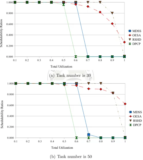
similar to that of DPCP, MDSS and RSHD. The schedulability ratios start to drop when the total utilizations are equal to 0.4, 0.5, 0.6 and 0.8 under DPCP, OESA, MDSS and RSHD, respectively. We can also observe that the performance of OESA is better than MDSS and DPCP in most situation. However, the performance of OESA algorithm is worse than that of RSHD when the total utilization of the system is less than 0.9. That is because Equation 3.5 of our OESA algorithm lets the utilization of DSP tasks become twice lager against the other algorithms. Therefore, the performance of OESA algorithm decays when the total utilization of the system is about equal to 0.5. However, although the point, where the schedulability ratios decreasing of our OESA algorithm is earlier than RSHD and MDSS, the decay ratio of our OESA algorithm is smoother and outperforms the others when the total utilization of the system is larger than 0.9. The reason can be concluded that because we use EDF-based scheduling algorithm as our method which is different from the compared RM-based algorithms, the schedulability upper bound of EDF-based algorithm is higher than that of RM-EDF-based algorithm. Moreover, the previous researches only take the total utilization including DSP activities as blocking time on GPP into account. Our proposed method separates the utilization calculation for the GPP and the DSP, respectively. Hence, our method is better when the system has a higher load. When the task number is equal to 50, the similar results can be obtained in Figure 4.1(b).
(a) Task number is 30
(b) Task number is 50
(a) ki,dsp= 0.8, ρ = 0.8 (b) ki,dsp= 0.2, ρ = 0.8
(c) ki,dsp = 0.8, ρ = 0.2 (d) ki,dsp= 0.2, ρ = 0.2
The Extended Experiment
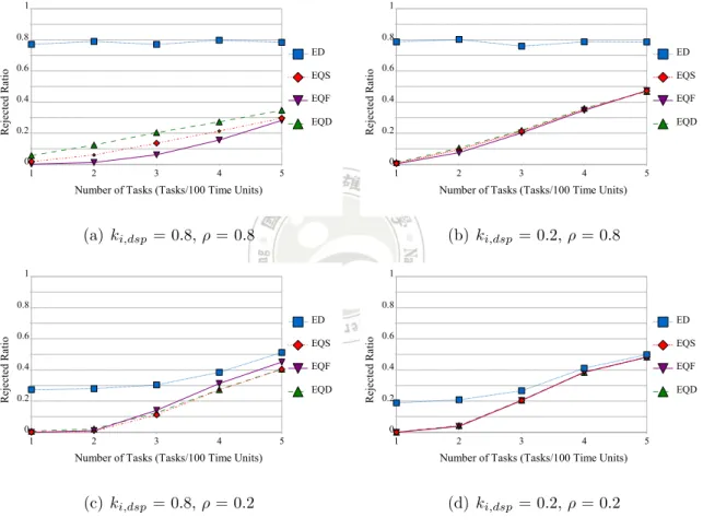
At the extended experiment, we compare four deadline assignment strategies under our method. The strategies are ED, EQS, EQF, and EQD. Figures 4.2(a), 4.2(b), 4.2(c), and 4.2(d) show the rejected ratios when ki,dsp= 0.8 and ρ = 0.8, ki,dsp= 0.2
and ρ = 0.8, ki,dsp = 0.8 and ρ = 0.2, and ki,dsp = 0.2 and ρ = 0.2, respectively.
From Figure 4.2(a), we can observe that the rejected ratio of ED strategy is always near 0.8. The reason is that ED strategy always assigns most of the relative deadline of the task to the subtask τi,pre if τi is a DSP task, and then it causes the admission
control test for the DSP to fail. Almost all DSP tasks are rejected. Thereby, its rejected ratio is close to the ρ value, i.e., 0.8. The similar results are shown in Figure 4.2(b), too. In addition, we can observe the EQF strategy outperforms the other strategies. Furthermore, because EQF strategy assigns relative deadlines to subtaks according to their execution requirements, it has better flexibility than the other compared strategies, i.e., ED, EQS, and EQD. As we know that EQS strategy assigns “slack” to subtasks fairly, and EQD strategy assigns “relative deadlines” of subtasks impartially. Consequently, EQF strategy has better performance than the others, and EQS strategy outperforms EQD strategy.
Moreover, the performance of EQD(/EQS) in Figures 4.2(b) and 4.2(d) is worse than that of EQD(/EQS) in Figure 4.2(a) and 4.2(c) on average. The reason is that for a DSP task τi when ki,dsp = 0.8 and ρ = 0.8, or ki,dsp = 0.8 and ρ = 0.2,
EQD(/EQS) strategy assigns the relative deadline to subtasks fairly and causes the utilization of subtask τi,dsp becomes larger (because ci,gpp is relatively smaller). On
the contrary, EQD(/EQS) strategy brings out the utilization of a DSP task on GPP larger when ki,dsp= 0.2 and ρ = 0.8, or ki,dsp = 0.2 and ρ = 0.2. As the twice larger
utilization caused by DSP tasks in Equation 3.5, the higher the utilization on GPP is, the worse the performance becomes. Furthermore, when there are more DSP tasks in the system, there are more tasks which cause the utilization of Equation 3.5 twice larger.
Another noticeable point is that the performance of EQF strategy is worse than EQS and EQD in Figure 4.2(c). It is because when ki,dsp = 0.8 and ρ = 0.2, the
ci,gpp of a DSP task is relatively smaller than ci,dsp. So the fair deadline assignment
comparatively. However, EQF strategy keeps the utilization of subtasks form im-balance. Equation 3.5, hence, is hard to pass for EQF strategy.
Besides, the performance differences among EQF, EQS and EQD in Figure 4.2(a) are larger than those in Figure 4.2(b), Figure 4.2(c) and Figure 4.2(d). It is because when ki,dsp = 0.2 and ρ = 0.8, ki,dsp = 0.8 and ρ = 0.2, and ki,dsp = 0.2 and ρ = 0.2,
Equation 3.5 has a higher probability of failure than that of Equation 3.6. When the load of the DSP is higher (i.e., the case where ki,dsp = 0.8 and ρ = 0.8), the
load on GPP is lighter relatively. The deadline assignment strategy which has larger flexibility such as EQF can affect the system more and the difference between those
deadline assignment strategies therefore is more obvious. Note that the rejected
ratio of EQF strategy increases faster than the other strategies just because DSP has already no adjustable spaces. In Figure 4.2(c) and Figure 4.2(d), ED strategy has the alike ratio as the value of ρ initially. It has the same reason of why ED strategy rejects tasks in Figure 4.2(a) initially. Nevertheless, the rejected ratio of ED strategy becomes worst as the task numbers increase against Figure 4.2(a) and Figure 4.2(b). The scheduler rejects sporadic tasks while the task numbers increases just because of not only the DSP tasks but also the regular tasks.
One more significant point is that EQD, EQS and EQF strategies have similar results in Figures 4.2(b), 4.2(c), and 4.2(d). It is due to the total utilization of GPP when ki,dsp= 0.2 and ρ = 0.8, ki,dsp = 0.8 and ρ = 0.2, and ki,dsp= 0.2 and ρ = 0.2
is higher than that when ki,dsp = 0.8 and ρ = 0.8. Therefore, there is no enough
adjustable flexibility for GPP. Hence, the rejected ratios of EQF, EQS and EQD are similar when ki,dsp = 0.2 and ρ = 0.8, ki,dsp = 0.8 and ρ = 0.2, or ki,dsp = 0.2 and
ρ = 0.2.
4.2.2
Integration with Total Bandwidth Server
The Total Bandwidth Server [19, 20] is dedicated to schedule aperiodic and sproadic tasks. The estimative threshold which decides a sporadic task can be inserted into the system or not is shown in Equation 4.3. WDA strategy can let users reave slacks of subtask on the DSP to subtasks on the GPP with the user-defined γ value. Thereby, more aperiodic and sporadic tasks on the GPP are capable of being accepted and scheduled.
Figure 4.3: Application of TBS where the system load is 0.7
Figure 4.3 shows the rejected ratios of sporadic tasks under the setting of different
γ values while the total utilization of the system is equal to 0.7. When γ = −0.1,
the rejected ratio is always close to 1. The reason is that when γ = −0.1, the rejected ratios is close to the upper bound of feasible range of γ such that there is no enough flexibility on the DSP to offer to the GPP. Therefore, there are nearly no new sporadic tasks that are able to be inserted into the system. Moreover, while the value of γ is set as −0.15 or −0.2, the rejected ratios is increased when the task arrival ratio of sporadic tasks is larger. The reason is because the load on the GPP has already fulfilled progressively and the newly-arrival sporadic task therefore fails to pass through the Equation 4.3. Compared with γ = −0.1, when γ = −0.15 or
−0.2, more slack of subtasks on the DSP is purloined. Therefore, the GPP has more
idle time to run sporadic tasks. Hence, the rejected ratio becomes smaller. The most significant point is that the feasible range of γ in Figure 4.3 is negative. It means the original schedulability test, without adjusting via γ, fails under the task sets (note that WDA strategy with γ = 0 is equivalent to EQF strategy). The WDA strategy
is a general case of EQF strategy and may fortunately help the schedulability tests succeed even if the tests fail initially.
As similar with Figure 4.3, Figure 4.4 has similar phenomenons. Moreover, while the task number is 5 or 10, the rejected ratios of γ = 0 and −0.05 have similar results in Figure 4.4. It is due to that although the set values of γ are close to the lower bound of feasible range of γ, the stolen slacks of subtasks on the DSP is enough so that the sporadic tasks could be accepted and scheduled by the system. Note that the feasible range of γ in Figure 4.4 has positive values, i.e. 0.1, and 0.05. It implies that we can steal slacks of subtasks on the DSP for subtasks on the GPP in an opposite manner according to the user requirement.
Figure 4.5 shows the schedulability ratios while using different γ values to adjust relative deadlines of subtasks. The experiment settings are the same as those for Figure 4.3. We can observe that under γ = 0 the schedulability ratio becomes zero when the total utilization is 0.7, i.e., if we use EQF strategy instead of WDA strategy, all the tested task sets fail in the schedulability test. However, most the tested task sets could pass the schedulability tests while we adjust the relative deadline via
Figure 4.5: Schedulability test under different γ values where Cmax = 1000, Dmin =
10000 and K = 0.1
between −0.9 and −0.2, which are derived based on Equations 3.12 and 3.13. The schedulability ratios get worse when γ is not in the range, e.g., γ = −0.3 in the figure.
Chapter 5
Conclusion and Future Work
In this thesis, we propose an online EDF-based scheduling algorithm, named OESA, which dynamically schedules real-time tasks in a heterogenous multiprocessor sys-tem. And then we add the concept of weighted deadline assignment to conduce to bias load balance and to apply to schedule sporadic tasks with Total Bandwidth Server. As the simulations results, we evaluate the performance of our method com-paring with MDSS, RSHD and DPCP. Moreover, we show the results of adding WDA strategy based on OESA at the second experiment and present an inductive conclusion and give some future work in this chapter. Besides, we address the situa-tion of scheduling a set of tasks in a heterogenous multiprocessor system composed of a general purpose processor and a DSP. To summarize our OESA algorithm and WDA strategy, there are some primary contributions listed below:
1. The equations of schedulability test which decide the system can obtain a feasible solution or not has been shown to have higher performance in our simulation results while the total system utilization is higher.
2. The schedulable upper bound is relaxed from 0.69 to 1.
3. Obtaining a better deadline assignment strategy in average case.
4. The results of achieving more load balance between GPP and DSP and letting some unschedulable system become schedulable with WDA strategy are also testified in the simulation results.
More than our features mentioned before, there are still some appealing prob-lems which are worthy to be investigated in the future, such as: Assigning relative
deadlines of subtasks via different γ according to their characteristics dynamically in runtime; Deriving a more accurate schedulability bound in this dual-cores het-erogenous multiprocessor system; Extending our OESA algorithm to deal with the condition where all the GPP and DSP have multiple cores.
Bibliography
[1] T. Wiegand, G. J. Sullivan, G. Bjontegaard, and A. Luthra, “Overview of the h.264/avc video coding standard,” IEEE Transactions on Circuits and Systems
for Video Technology, vol. 13, pp. 560–576, July 2003.
[2] M. Bosi, K. Brandenburg, S. Quackenbush, L. Fielder, K. Akagiri, H. Fuchs, M. Dietz, J. Herre, G. Davidson, and Y. Oikawa, “ISO/IEC MPEG-2 advanced audio coding,” Journal of the Audio Engineering Society, vol. 45, pp. 789–814, 1997.
[3] “TMS320DM6446 Digital Media System-on-Chip – Datasheet.” Texas Instru-ments, 31 Mar 2008.
[4] M. Pelleh, “A study of real time scheduling for multiprocessor systems,” in
Proc. IEEE 24th Convention of Electrical and Electronics Engineers in Israel,
pp. 295–299, Nov. 2006.
[5] J. Goossens, S. Funk, and S. Baruah, “Priority-driven scheduling of periodic task systems on multiprocessors,” Real-Time System, vol. 25, no. 2-3, pp. 187– 205, 2003.
[6] T. P. Baker, “Multiprocessor edf and deadline monotonic schedulability analy-sis,” in Proc. 24th IEEE Real-Time Systems Symposium RTSS 2003, pp. 120– 129, 2003.
[7] T. P. Baker, “An analysis of edf schedulability on a multiprocessor,”
Transac-tions on Parallel and Distributed Systems, vol. 16, pp. 760–768, Aug. 2005.
[8] S. K. Baruah, “The non-preemptive scheduling of periodic tasks upon multi-processors,” Real-Time System, vol. 32, pp. 9–20, Feb 2006.
[9] S. Dolev and A. Keizelman, “Non-preemptive real-time scheduling of multime-dia tasks,” in Proc. Third IEEE Symposium on Computers and
Communica-tions ISCC ’98, pp. 652–656, 30 June–2 July 1998.
[10] C. Lee, J. Lehoczky, D. Siewiorek, R. Rajkumar, and J. Hansen, “A scalable solution to the multi-resource qos problem,” in Proc. 20th IEEE Real-Time
Systems Symposium, pp. 315–326, 1–3 Dec. 1999.
[11] K. Kim, D. Kim, and C. Park, “Real-time scheduling in heterogeneous dual-core architectures,” in Proc. 12th International Conference on Parallel and
Dis-tributed Systems ICPADS 2006, vol. 2, p. 6pp., 12–15 July 2006.
[12] P. Gai, L. Abeni, and G. Buttazzo, “Multiprocessor dsp scheduling in system-on-a-chip architectures,” in Proc. 14th Euromicro Conference on Real-Time
Systems, pp. 231–238, 19–21 June 2002.
[13] L. Sha, R. Rajkumar, and J. P. Lehoczky, “Priority inheritance protocols: an approach to real-time synchronization,” IEEE Transactions on Services
Com-puting, vol. 39, pp. 1175–1185, Sept. 1990.
[14] C. L. Liu and J. W. Layland, “Scheduling algorithms for multiprogramming in a hard-real-time environment,” Journal of the ACM JACM 1973, vol. 20, no. 1, pp. 46–61, 1973.
[15] P. G. Paulin, C. Pilkington, M. Langevin, E. Bensoudane, O. Benny, D. Lyon-nard, B. Lavigueur, and D. Lo, “Distributed object models for multi-processor soc’s, with application to low-power multimedia wireless systems,” in DATE
’06: Proceedings of the conference on Design, automation and test in Europe,
(3001 Leuven, Belgium, Belgium), pp. 482–487, European Design and Automa-tion AssociaAutoma-tion, 2006.
[16] B. Kao and H. Garcia-Molina, “Deadline assignment in a distributed soft real-time system,” IEEE Transactions on Parallel and Distributed Systems, vol. 8, pp. 1268–1274, Dec. 1997.
[17] J. M. L´opez, J. L. D´ıaz, and D. F. Garc´ıa, “Utilization bounds for edf scheduling on real-time multiprocessor systems,” Real-Time System, vol. 28, no. 1, pp. 39– 68, 2004.
[18] J. W. S. Liu, Real-Time Systems. Prentice Hall, 2000.
[19] Z. Deng, J.-S. Liu, and J. Sun, “A scheme for scheduling hard real-time applica-tions in open system environment,” in Real-Time Systems, 1997. Proceedings.,
Ninth Euromicro Workshop on, pp. 191–199, Jun 1997.
[20] M. Spuri and G. Buttazzo, “Scheduling aperiodic tasks in dynamic priority systems,” Real-Time System, vol. 10, pp. 179–210, Mar. 1996.