合作式學習為基礎之混合型進化演算法在模糊類神經系統設計及多漏斗函數最佳化的應用

國 立 交 通 大 學

電控工程研究所

博士論文

合作式學習為基礎之混合型進化演算法在模糊類神

經系統設計及多漏斗函數最佳化的應用

Cooperative Learning Based Hybrid Evolutionary Algorithms

for Neural Fuzzy System Design and Optimization of

Multi-funnel Functions

研究生：鄭逸章

指導教授：林昇甫 博士

合作式學習為基礎之混合型進化演算法在模糊類神

經系統設計及多漏斗函數最佳化的應用

Cooperative Learning Based Hybrid Evolutionary Algorithms

for Neural Fuzzy System Design and Optimization of

Multi-funnel Functions

研 究 生：鄭逸章

Student: Yi-Chang Cheng

指導教授：林昇甫 博士

Advisor:

Dr.

Sheng-Fuu

Lin

國 立 交 通 大 學

電機與控制工程學系

博 士 論 文

A Dissertation

Submitted to Institute of Electrical Control Engineering

National Chiao Tung University

In Partial Fulfillment of the Requirements

For the Degree of

Doctor of Philosophy

in

Electrical and Control Engineering

June 2012

Hsinchu, Taiwan, Republic of China

中華民國一○一年六月

合作式學習為基礎之混合型進化演算法在模糊類神

經系統設計及多漏斗函數最佳化的應用

研究生：鄭逸章 指導教授：林昇甫 博士

國立交通大學 電控工程研究所

摘 要

在這篇論文中，我們主要在探討的是進化型演算法的合作學習機制。本論文中所探討的 三種進化型演算法包括：基因演算法、粒子群聚最佳化演算法、以及自適應共變異數矩 陣演化策略。在基因演算法的改良上，我們提出了族群式的共生演化概念，使得基因演 算法可以將解空間分割成數個子空間，且在每個子空間中分別得去探索最佳解。我們也 在合作式的粒子群聚演算法中提出了一個可分割度的偵測方法，以便將不可分割之變數 置入同一族群中演化。至於關於自適應共變異數矩陣演化策略的改良，本論文提出了一 個基於均值移動的平行運算機制，使得我們可以平行地在解空間中提供多個自適應共變 異數矩陣演化策略學習器來探索解空間中的不同區域。論文的內容包括了將進化型演算 法套用在模糊類神經系統上之架構和參數學習、演算法上的改良、平行運算機制以及結 合兩種演算法優點的混合型演算法的研究。 關鍵字：合作式學習，基因演算法，粒子群聚最佳化演算法，演化策略，自適應共變異 數矩陣。

Cooperative Learning Based Hybrid Evolutionary Algorithms

for Neural Fuzzy System Design and Optimization of

Multi-funnel Functions

Student：Yi-Chang Cheng Advisor：Dr. Sheng-Fuu Lin

Institute of Electrical Control Engineering

National Chiao Tung University

Abstract

In this dissertation, we mainly focus on researching the cooperative behavior of evolutionary algorithms. Algorithms discussed in this dissertation include genetic algorithm (GA), particle swarm optimization (PSO) and evolution strategy with covariance matrix adaptation (CMA-ES). The modification of genetic algorithm (GA) is done by introducing the group-based symbiotic evolution (GSE) technique which enables genetic algorithm (GA) to partition the search space into smaller subspaces and explore each smaller subspace by a separate agent to alleviate the curse of dimensionality. We also propose a separability detection method based on covariance matrix adaption mechanism into the cooperative particle swarm optimization (CPSO) to locate non-separable variables into the same swarm. As to the research of evolution strategy with covariance matrix adaptation (CMA-ES), we introduce the mean shift procedure which allows us to apply multiple CMA-ES instances to explore different parts of the search space in parallel. The scope of this dissertation includes how to implement evolutionary algorithms on neural-fuzzy systems, the improvement of algorithms, parallel computing and the emergence of two algorithms

Keywords: cooperative learning, genetic algorithm, particle swarm optimization, evolution

誌謝

經過六年的奮戰，博士生涯終告一段落，這六年，需要感謝的人太多，因為攻讀博 士學位又豈是易事，若不是有這麼多貴人相助與支持，怎有辦法成就今日。 家人，往往是最好的避風港，感謝父親鄭文昌先生、母親羅鳳美女士如此無怨無悔 的付出，沒有您們的支持，我無法辦到，身為您們兒子，實在太幸福了；相對於您們的 付出，我並不是個稱職的好兒子，總在實驗室忙到沒日沒夜，為了學業的繁忙而忘了關 心，照顧您們，卻從未聽您們抱怨，甚至在經濟上如此的資助我，謝謝您們，您們是我 永遠的靠山，而將來我也會努力，成為您們的靠山。弟弟鄭彥章先生，感謝你的體諒； 如此漫長的求學，父親母親都靠你們照顧，辛苦了。 指導教授是博士論文產生最重要的ㄧ環，我的指導教授-林昇甫博士，感謝您指導 學生，在您的教導下，學生學習到很多，您在學術研究上的身教、言教，讓學生的博士 生活能無比的充實，也增加了多元的歷練。 博士論文的完善需要口試委員的監督指導，感謝我的口試委員—潘晴財教授、林錫 寬教授、張翔教授以及鍾鴻源教授，感謝您們不辭辛勞不遠千里而來，也感謝您們指導 學生口試，有了您們的指導，學生的博士論文才能更臻完備。 研究室裡互相扶持幫忙的好友太多了，謝謝你們。特別感謝實驗室博士班學長永 吉，同學啟曜及俊偉，有你們的並肩作戰，博士生涯才不致如此漫長。另外也特別感謝 碩士班學弟煒清，你是一個很好的學習夥伴，感謝你的協助，此博士論文才能順利完成， 辛苦了。 在此，僅將此論文獻給我最愛的家人、師長、學長、同學、學弟妹，願與大家分享 這難得的榮耀。 鄭逸章 一○一年 六月 五日

Contents

CHINESE ABSTRACT... I ABSTRACT ...II CHINESE ACKNOWLEDGEMENTS ... III CONTENTS...IV LIST OF TABLES ...VI LIST OF FIGURES... VII

CHAPTER 1 INTRODUCTION... 1

1.1MOTIVATION... 1

1.2RELATED WORKS... 4

1.2.1 Reinforcement Learning Tasks... 4

1.2.2 Multi-funnel Function Optimization Functions ... 7

1.3APPROACH... 10

1.4ORGANIZATION OF DISSERTATION... 11

CHAPTER 2 FOUNDATIONS ... 13

2.1NEURAL FUZZY SYSTEM... 13

2.2GENETIC ALGORITHM... 16

2.3PARTICLE SWARM OPTIMIZATION... 18

2.3.1 Standard Particle Swarm Optimization... 18

2.3.2 Cooperative Particle Swarm Optimization ... 20

2.4EVOLUTION STRATEGY WITH COVARIANCE MATRIX ADAPTATION... 22

2.4.1 Standard CMA-ES... 22

2.4.2 Kernel Density Estimation ... 24

2.4.3 Mean Shift Procedure ... 26

CHAPTER 3 EVOLUTIONARY ALGORITHMS... 29

3.1Q-VALUE BASED PSO... 29

3.1.1 Learning Q-values of Particles... 30

3.2.2 Q-value based PSO... 31

3.2TWO-STRATEGY REINFORCEMENT EVOLUTIONARY ALGORITHM... 33

3.2.1 Two-strategy Reinforcement Signal Design ... 33

3.3.1 Motivation ... 38

3.3.2 Sampling from a Mixture Model ... 41

3.3.3 Mean Shift-based Clustering ... 41

3.3.4 Updating of Mixture Probability Model ... 45

3.4ASEPARABILITY DETECTION APPROACH TO COOPERATIVE PARTICLE SWARM OPTIMIZER... 48

CHAPTER 4 SIMULATIONS ... 51

4.1REINFORCEMENT LEARNING TASKS... 51

4.2REAL-VALUED FUNCTION OPTIMIZATION TASK... 78

4.2.1 Test Functions Introduction ... 79

4.2.2 Function Optimization Simulation... 81

CHAPTER 5 CONCLUSION... 89

BIBLIOGRAPHY ... 92

VITA ... 100

PUBLICATION LIST ... 101

List of Tables

Table 4.1: The initial parameters of the QPSO for cart-pole balancing system...54

Table 4.2 : The initial parameters of the TSR-EA for cart-pole balancing system. ...55

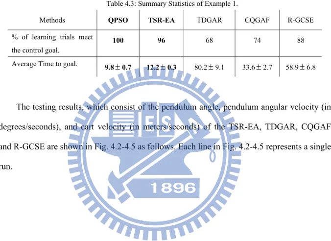
Table 4.3: Summary Statistics of Example 1. ...56

Table 4.4: Summary Statistics of Example 1 under a difficult control goal. ...61

Table 4.5: The initial parameters of the QPSO for two-pole inverted pendulum system. ...66

Table 4.6 : The initial parameters of the TSR-EA for two-pole inverted pendulum system...67

Table 4.7: Summary Statistics of Example 2. ...68

Table 4.8: Type and name of test functions. ...79

Table 4.9: Parameters of the simulation...82

Table 4.10: MS-CMA-ES and CMA-ES parameters...83

Table 4.11: Average fitness at 20% number of fitness calculations...84

Table 4.12: Average fitness at 50% number of fitness calculations...84

Table 4.13: Average fitness at 100% number of fitness calculations...85

List of Figures

Figure 1.1: Visualization of a single-funnel, 2-D Rastrigin’s function. ...7

Figure 1.2: Visualization of a multi-funnel-funnel, 2-D double Rastrigin’s function. ...7

Figure 2.1: Structure of TSK-type NFS...15

Figure 2.2: Flowchart of the genetic algorithm. ...16

Figure 2.3: The roulette wheel selection. ...17

Figure 2.4: Crossover operator. ...17

Figure 2.5: Mutation operator...18

Figure 2.6: Diagram of the PSO learning mechanism...19

Figure 2.7: Flowchart of the PSO...21

Figure 2.8: Schematic diagram of the CPSO...21

Figure 3.1: Architecture of QPSO. ...30

Figure 3.2: Coding scheme between a particle and a TSK-type NFS in QPSO...32

Figure 3.3: Block diagram of QPSO. ...32

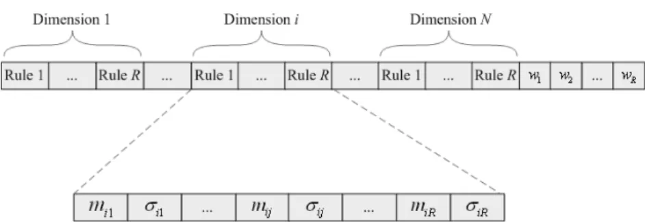
Figure 3.4: Structure of a chromosome in the GSE...37

Figure 3.5: Coding structure of a chromosome in the TSR-EA. ...37

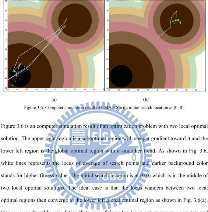
Figure 3.6: Computer simulation result of CMA-ES with initial search location at (0, 0). ....39

Figure 3.7: The block diagram of the MS-CMA-ES. ...40

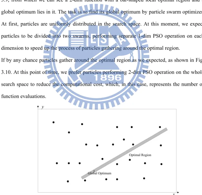
Figure 3.8: Example of kernel density estimation with variable bandwidth selection...46

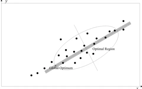
Figure 3.9: Case with particles uniformly distributed in the search space to find the global optimum lies in a bar-shaped local optimal region...48

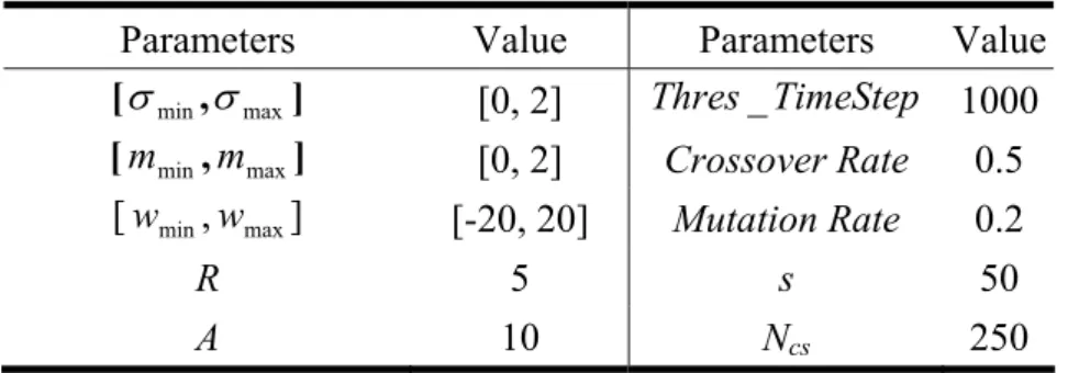
Figure 3.10: Case with particles gather around the bar-shaped optimal region to find the global optimum...49

Figure 3.11: Block diagram of SD-CPSO. ...50

Figure 4.1: Single-link inverted pendulum system. ...52

Figure 4.2: 50 control results of the cart-pole balancing system using the TSR-EA in Example 1. (a) Angle of the pendulum. (b) Angular velocity of the pendulum. (c) Velocity of the cart. ...57

Figure 4.3: 50 control results of the cart-pole balancing system using the TDGAR in Example 1. (a) Angle of the pendulum. (b) Angular velocity of the pendulum. (c) Velocity of the cart. ...58

Figure 4.4: 50 control results of the cart-pole balancing system using the CQGAF in Example 1. (a) Angle of the pendulum. (b) Angular velocity of the pendulum. (c) Velocity of the cart. ...59 Figure 4.5: 50 control results of the cart-pole balancing system using the R-GCSE in Example

cart. ...60

Figure 4.6: 50 first 1000 time steps control results the QPSO of the cart-pole balancing system. . (a) Angle of the pendulum. (b) Angular velocity of the pendulum. (c) Velocity of the cart. ...62

Figure 4.7: 50 last 1000 time steps control results the QPSO of the cart-pole balancing system. . (a) Angle of the pendulum. (b) Angular velocity of the pendulum. (c) Velocity of the cart. ...63

Figure 4.8: Double-link inverted pendulum system. ...64

Figure 4.9: 50 first 1000 time steps control results of the double-link inverted pendulum system using the QPSO. (a) Angle of link 1. (a) Angle of link 2. (c) Angular velocity of link 1. (d) Angular velocity of link 2...70

Figure 4.10: 50 first 1000 time steps control results of the double-link inverted pendulum system using the TSR-EA. (a) Angle of link 1. (a) Angle of link 2. (c) Angular velocity of link 1. (d) Angular velocity of link 2...71

Figure 4.11: 50 first 1000 time steps control results of the double-link inverted pendulum system using the TDGAR. (a) Angle of link 1. (a) Angle of link 2. (c) Angular velocity of link 1. (d) Angular velocity of link 2...72

Figure 4.12: 50 first 1000 time steps control results of the double-link inverted pendulum system using the CQGAF. (a) Angle of link 1. (a) Angle of link 2. (c) Angular velocity of link 1. (d) Angular velocity of link 2...74

Figure 4.13: 50 first 1000 time steps control results of the double-link inverted pendulum system using the R-GCSE. (a) Angle of link 1. (a) Angle of link 2. (c) Angular velocity of link 1. (d) Angular velocity of link 2...75

Figure 4.14: 50 last 1000 time steps control results of the double-link inverted pendulum system using the QPSO. (a) Angle of link 1. (b) Angular velocity of link 1. (c) Angle of link 2. (d) Angular velocity of link 2...77

Figure 4.15: 50 last 1000 time steps control results of the double-link inverted pendulum system using the TSR-EA. (a) Angle of link 1. (b) Angular velocity of link 1. (c) Angle of link 2. (d) Angular velocity of link 2...78

Figure 4.16: Contour details of double-Rastrigin function. ...80

Figure 4.17: Graph of global search ability test of (a) CMA-ES. (b) MS-CMA-ES. ...81

Fugure 4.18: Visualization of a 2-D Michalewicz's function. ...88

Figure 4.19: Computer simulation results of applying Michalewicz's function in its (a) unrotated form, (b) rotated form...88

CHAPTER 1

INTRODUCTION

Evolutionary algorithms [1]-[6] are stochastic, population-based optimization learning algorithms that can be applied to a wide range of problems. Generally speaking, there is no clear rank between different evolutionary algorithms. We can only say that certain algorithm is more applicable than others to certain optimization problems. In this dissertation, we apply the modified version of genetic algorithm (GA) [7] and particle swarm optimization (PSO) [8]-[10] to high-dimensional, reinforcement learning tasks, and apply evolution strategy with covariance matrix adaptation (CMA-ES) [11]-[13] to complex, low-dimensional real-valued function optimization tasks.

1.1 Motivation

Evolutionary algorithms are discovered through simulating some social behavior, such as the bird flocking, the recombination or the mutation of genes. Normally, evolutionary algorithms maintain a population of potential solutions to some optimization problem, generating new solutions at each iteration by using a variety of corresponding operators. Their learning procedures take place in populations made of individuals with specific behaviors similar to certain biological phenomena. Individuals keep exploring the solution space and exploiting information between individuals while evolution proceeding. In general, by means of exploring and exploiting, evolutionary algorithms are less likely to be trapped at the local optimum.

Evolutionary algorithms are applicable to a wide range of problems, including training neural-fuzzy systems (NFS) [14]-[17], reinforcement learning control [18]-[22] and complex, multi-funnel [23]-[26] function optimization tasks. However, as with GA, PSO and CMA-ES,

nearly every other kind of stochastic optimization algorithms suffer from the “curse of dimensionality,” which simply put, implies that their performance deteriorates as the dimensionality of the search space increases. One way to overcome this difficulty is to partition the search space into lower dimensional subspaces, as long as the optimization algorithm can guarantee that it will be able to search every possible region of the search space. Van den Bergh and Engelbrecht suggested that the search space should be partitioned by splitting the solution vectors into smaller vectors and proposed a cooperative approach to particle swarm optimization (CPSO) [27]-[28]. Each of these smaller search spaces is then searched by a separate PSO instance; the fitness function is evaluated by combining solutions found by each swarm of the PSO instance. In this dissertation, we introduce the cooperative learning behavior to GA and proposed the groups-based symbiotic evolution (GSE) [29]. The proposed GSE is applied to training a NFS. It is different from traditional symbiotic evolution where each population in the GSE is divided to several groups and each group represents a set of chromosomes that belongs to one fuzzy rule. The fitness value of each fuzzy rule can be evaluated locally. However, separating the search space also arouses two issues.

The first issue is the possibility that the partitioning could lead to the introduction of pseudooptimum, which means that the combination of optima found by each learning instance may not be an actual optimum point to the original search space, may not even be a local optimum point. In [27], Van den Bergh and Engelbrecht proposed a variation of CPSO called the CPSO-HK to alleviate the issue of pseudooptimum. The CPSO is one of the most

significant improvements to the standard PSO. Algorithm CPSO-HK is a hybrid from the

standard PSO and the CPSO-SK model. It prevents the solution found so far from becoming a pseudooptimum by executing the CPSO-SK algorithm for one iteration, followed by one

iteration of the PSO algorithm. Computer simulations in [27] have shown that the CPSO-HK

among parameters.

The second issue aroused by partitioning the search space is that performances of the cooperative learning algorithms deteriorate when correlated variables are placed into separate populations. In this dissertation, we call such variables “non-separable.” A function f is said to be separable if

1 1 1 1

( , , )

arg min ( , , ) (arg min ( , ), ,arg min ( , ))

n n n n

x x f x x = x f x x f x , (1.1)

and it is followed by a fact that f can be optimized in a sequence of n independent 1-D optimization processes. In this dissertation, we propose a separability detection approach based on covariance matrix adaptation to find non-separable variables so that they can previously be placed into the same swarm to address the difficulty that the original CPSO encounters. This proposed variation on the original CPSO to detect the separability of the variables is called the SD-CPSO [106]. The SD-CPSO helps the CPSO self-organize the swarms composed of non-separable variables. In order to implement this idea, we have to determine the timing of switching between the PSO and the CPSO operation when dealing with a task. In this dissertation, we think this can be done by determining the separability between variables, and placing non-separable into the same swarm at each generation. If at certain moment, all variables are determined as non-separable, then the PSO operation is taken; otherwise, the CPSO operation is taken. The separability between variables is found by estimating the covariance matrix of the distribution of particles. The mechanism we adopt is the covariance matrix adaptation proposed from evolution strategy with covariance matrix adaption (CMA-ES) [11]-[13]. Conventionally, there exists a contradiction between the local search performance and the global exploration power of a learning algorithm [32]. For example, the GA and PSO are noted for their great global exploration power; whereas, due to the adaptivity of the local search, the CMA-ES owns an outstanding local search performance. In this dissertation, we apply the GA and PSO to high-dimensional, reinforcement learning

tasks, and apply the CMA-ES to complex, mid-dimensional real-valued function optimization tasks.

1.2 Related Works

In this dissertation, we basically encode parameters on a NFS into individuals of GA or PSO to perform reinforcement learning control, and apply a parallel learning structured version of CMA-ES to complex, multi-funnel function optimization. As a result, we will discuss these two types of optimization tasks in this section. The discussion of reinforcement learning will be shown in section 1.2.1 and the discussion of multi-funnel function optimization will be shown in section 1.2.2.

1.2.1 Reinforcement Learning Tasks

In recent years, the application of NFS in control engineering has become a popular research topic [33]-[43]. In general, the way of tuning the parameters on a NFS can be divided into two categories: supervised learning [44] and reinforcement learning [18].

Supervised learning is a machine learning technique for updating its parameters from training data. The training data is composed of pairs of inputs, and desired outputs. The object of the supervised learning is to predict the output value of the NFS for any valid input data after its parameters have been trained by a number of training data. However, for many control tasks, training data are usually difficult or too costly, or even not accessible. As a result, reinforcement learning is more practicable than supervised learning in many occasions.

In reinforcement learning, the agent receives from its environment a reinforcement signal at each time step. This signal could be either a reward or a punishment. Meanwhile, the agent explores actions from the action set, and finds out which action yields the greatest reward. To solve reinforcement problem, temporal difference (TD) [19]-[21] is one of the most common

method. In TD learning, learners don’t have to wait until the end of a trial; instead, TD methods need wait only one time step. This is crucial for applications that have very long trials or tasks that are continuous and have no trials at all. Q-learning [22] is a powerful and easy-implementing TD-based approach. It is a reinforcement learning technique that works by updating a simple action-value iteration function. This function gives the measurement of taking a given action in a given state.

Besides TD methods, many evolutionary algorithms such as PSO, GA, evolutionary programming [45], and evolution strategies [46] are popular for solving reinforcement learning tasks. These learning procedures are based on populations made of individuals with specific behaviors similar to certain biological phenomena. Individuals keep exploring the solution space and exploiting information between individuals while evolution proceeding. In general, by means of exploring and exploiting, evolutionary algorithms are less likely to be trapped at the local optimum. Many researches on using evolutionary algorithm for solving reinforcement learning tasks have been proposed recently [47]-[50]. In [49], authors propose a swarm intelligence based reinforcement learning (SWIRL) method to train artificial neural networks (ANN). Authors apply ant colony optimization to select ANN topology and apply the PSO to adjust ANN connection weights. In [50], Lin and Hsu present a reinforcement hybrid learning algorithm (R-HELA) combining the compact GA (CGA) [51] and the modified variable-length GA (VGA) [52] on recurrent wavelet-based NFS. A counter is used to accumulate the time steps until the control task fails and the accumulated values are fed into individuals as fitness functions. Lin and Hsu’s model is very effective; however, its fitness function only indicates how long can the controller work well instead of measuring how soon the system can meet the control goal, which is also very important in reinforcement learning. There is also a growing interest in combining the advantages of evolutionary algorithms and TD-based reinforcement learning [53]-[54]. In [53], a TD and GA based reinforcement learning (TDGAR) is proposed. Authors propose a neural structure composed

of two feedforward networks for reinforcement learning, the critic network and the action network. The critic network predicts the external signal provides a more informative internal signal to the action network. The action network uses GA to determine the output of the learning system. The weight update rule for the hidden layer of the critic network is based on error backpropagation. In [54], an on-line clustering and Q-value based GA reinforcement learning for fuzzy system (CQGAF) is proposed. In one generation CQGAF learning, one individual is applied to the environment to estimate the fitness function, Q-value, and Q-values of other individuals are updated by eligibility trace. The GA operation is performed by the end of each trial and creates a new generation of individuals. In [55], authors proposed a recurrent wavelet-based NFS with a reinforcement group cooperation-based symbiotic evolution (R-GCSE) algorithm. In [55], a population is divided to several groups. The R-GCSE has a good ability of parameter learning by adopting the concept that each group formed by a set of chromosomes cooperates with other groups to generate better chromosomes.

Although the aforementioned reinforcement learning methods work well in many applications, there is an issue remains to be solved. No fitness function in these methods indicates how soon the learning agents can control the system's state into a set of goal states. Sure there is no need to define the fitness function that way if there is no guidance provided to the controller of how to maintain the system's state in a desired operating range. As a result, in this dissertation, we proposed a Q-value based particle swarm optimization (QPSO) [56] which adopts the concept of Lyapunov design [57] for constructing safe reinforcement learning agents, and a GA based learning method called two-strategy reinforcement evolutionary algorithm (TSR-EA) [29] to solve reinforcement learning tasks. In both algorithms proposed in this dissertation, we manipulate our fitness function so that it can indicate how soon the controller achieves its control goal.

1.2.2 Multi-funnel Function Optimization Functions

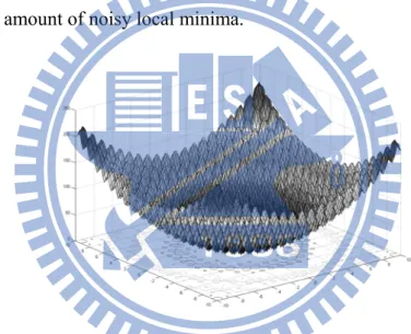
Normally, continuous function optimization problems are categorized into convex (unimodal) and non-convex (multimodal) functions. In this dissertation, we classified optimization problems into single-funnel and multi-funnel problems and we mainly focus on the optimization of multi-funnel functions. The difference between single- and multi-funnel functions can be illustrated by the following two figures, where Fig. 1.1 shows a visualization of a 2-D Rastrigin’s function, from which we can see that in spite of the large amount of local minima, there exists a trend to the global minimum. Figure 1.2 shows a visualization of a 2-D double Rastrigin’s function, from which we can see that there are two funnel-type global trends and a large amount of noisy local minima.

Figure 1.1: Visualization of a single-funnel, 2-D Rastrigin’s function.

A function is said to be single-funnel, even though it is highly multi-modal, if its local optima is structured such that there exists a global trend toward the best solution [58]. However, there are several real-world applications do not have this simple structure. Many optimization problems are characterized by their local optima distributing in separate clusters within the search space and there is no underlying convex topology toward their global optima. Problems of this type are referred to as multi-funnel functions [23]. Prominent examples for such applications include potential energy surfaces of biomolecules [24] and protein aggregation and misfolding [25]. It has been suggested that the global topology of a problem may have a strong influence on the performance of optimization of multi-funnel functions [26]. To this end, we introduce the mean shift procedure [59] into the evolution strategy with covariance matrix adaptation (CMA-ES) which allows us to apply multiple CMA-ES instances to explore different parts of the search space in parallel.

The CMA-ES has been proven to be among the most successful optimization algorithms for optimization of non-convex functions. During exploring of the search space, the CMA-ES generates a population of samples from a multivariate Gaussian distribution. The mean and covariance matrix of the sampling distribution are continuously adapted in order to improve the search direction and the sampling distribution. Recent improvements include a local restart CMA-ES (LR-CMA-ES) [60], which greatly prevents CMA-ES from being trapped into local optima, and a CMA-ES with iteratively increasing population size (IPOP-CMA-ES) [61], achieving excellent performance on non-convex, high-dimensional optimization problems. However, Hansen and Kern [62] have pointed out that on multi-funnel functions, where local optima cannot be interpreted as perturbations to an underlying convex (unimodal) topology, performance can strongly be limited. This could be due to the fact that CMA-ES was originally proposed as a local search strategy, whereas the concept of multi-funnel functions is intrinsically based on global information. As a result, some researches [26, 63]

exploration power. In [63], a particle swarm guided evolution strategy (PSGES) is proposed. Computer simulation results have shown that PSGES improves the original evolution strategy but is inferior to LR-CMA-ES and IPOP-CMA-ES. This could be due to a lack of local adaptivity mechanism. In [26], authors propose a particle swarm CMA-ES (PS-CMA-ES), which combines the local search performance of the CMA-ES with the global exploration power of the PSO. Computer simulation results in [26] have shown that no salient improvement over LR-CMA-ES and IPOP-CMA-ES on optimization of unimodal, basic multimodal functions, but improvement can be seen in optimization of high-dimensional multi-funnel functions. However, in spite of the great performance the PS-CMA-ES achieves, this methodology tends to be computationally expensive and the criterion of how frequent the PSO updates can be performed is not straightforward. In this dissertation, our objective is to improve performance on multi-funnel problems on one hand, and on-line determine the number of the CMA-ES instances on the other. Instead of directly combing the CMA-ES with certain “global” evolutionary algorithm, we introduce a computational module based on mean shift procedure into the CMA-ES. Mean shift procedure is a density estimation-based, non-parametric mode detection and clustering approach toward feature space analysis [59, 64, 65]. It determines the number of modes in a unknown probability density function (p.d.f.), and the density estimation is completed by kernel density estimator [66].

First, we apply kernel density estimation to the candidate solutions sampled by the CMA-ES. Then, we use the mean shift-based mode detection to determine the number of CMA-ES instances for exploring the search space simultaneously. In cases of more than one CMA-ES instances are applied, the proposed mean shift based evolution strategy with covariance matrix adaption (MS-CMA-ES) samples a population of candidate solutions from a mixture model of Gaussian distribution [67]. The covariance matrix of the mixture Gaussian sampling distribution is formed by the linear combination of the covariance matrixes of separate CMA-ES instances. Enforcing a mixture model provides a communication between

different CMA-ES instances such that the CMA-ES instances with better search locations can sample more offspring, while the CMA-ES instances trapped in local optima can fade out. Another advantage of the proposed MS-CMA-ES is that there is no requirement of the criterion for the fusion (or division) of the CMA-ES instances, nor does the predefinition of the number of CMA-ES instances as a parameter. The bandwidth of the kernel density estimator can also be computed through kernel smoothing [68]. The only extra parameter besides the original parameters of the CMA-ES is the learning rate of mixture weightings for mixture Gaussian components, which reduces challenges of applying our methodology.

In this dissertation, we compare the proposed MS-CMA-ES with the standard CMA-ES [13], some of its improvements [60, 61], and some hybrid algorithms that combine the evolution strategy with the PSO [26, 63]. Computer simulation results will show that the MS-CMA-ES has better performance in optimizing multi-funnel functions.

1.3 Approach

In this dissertation, four major algorithms are proposed. The first two algorithms are called Q-value based particle swarm optimization (QPSO) and two-strategy reinforcement evolutionary algorithm (TSR-EA) respectively. These two algorithms are both proposed to solve reinforcement learning tasks. The advantages of the QPSO can be shown from that it provides an alternative for Q-learning to solve reinforcement learning problem in one hand, and it extends the applicability of the PSO into reinforcement environment on the other. It also provides a reliable initial learning performance due to the Lyapunov design of learning agents. But one drawback of the QPSO is that it requires additional priori knowledge. The main advantages of the TSR-EA can be summarized as follows: 1) the proposed TSR mechanism enables us to evaluate a learning trial for both how long can the controller work under operating range instead of measuring how soon the system meet the control goal; 2) the

GSE is proposed to evaluate the fuzzy rule locally. However, in the TSR-EA, divide parameters corresponding to different fuzzy rule into separate groups is very straightforward. However, in the optimization task, if the correlation between parameters is unknown, placing uncorrelated parameters into a same group would be a challenge.

The third algorithm proposed in this dissertation is a separability approach to cooperative particle swarm optimization (SD-CPSO), and it is mainly proposed to help placing uncorrelated variables into a same swarm. The proposed separability detection approach is based on the CMA-ES.

The fourth algorithm proposed in this dissertation is the mean shift-based evolution strategy with covariance matrix adaptation (MS-CMA-ES). The introduced mean shift procedure provides functions of mode detection and clustering which allows us to apply multiple CMA-ES instances to explore different parts of the search space in parallel. The global exploration power of the standard CMA-ES is enhanced by the concept that each instance forms a separate CMA-ES agent to explore different parts of the search space. We evaluate the performance of the MS-CMA-ES on the optimization of multi-funnel functions and the new MS-CMA-ES algorithm shows superior performance on it.

1.4 Organization of Dissertation

The dissertation is arranged as follows.

Chapter 1 introduces the motivation, related work, approach, and organization of the dissertation.

Chapter 2 provides the fundamental information used in the dissertation. The foundation includes neural fuzzy network, genetic algorithm, standard and cooperative PSO, mean shift procedure and CMA-ES.

In Chapter 4, two types of computer simulations, reinforcement learning control tasks and multi-funnel optimization functions, are performed to verify the performance of the proposed algorithms. We apply QPSO and TSR-EA to two reinforcement learning control tasks, cart-pole balancing system and two-pole inverted pendulum control. The SD-CPSO and MS-CMA-ES are applied to real-valued function optimization tasks.

In Chapter 5, the conclusions, contribution, and future works of the dissertation are discussed.

CHAPTER 2

FOUNDATIONS

The background material and literature review that relates to the major components of the research purpose outlined above (neuro-fuzzy controller, genetic algorithm, particle swarm optimization, and evolution strategy with covariance matrix adaptation) are introduced in this chapter. The concept of neuro-fuzzy controller is discussed in the first section. The concept of genetic algorithm (GA) is introduced in Section 2.2. In Section 2.3, the concept of particle swarm optimization (PSO) and some of its improvements are discussed. The final section focuses on some background knowledge related to the proposed mean shift-based evolution strategy with covariance matrix adaptation (MS-CMA-ES), such as kernel density estimation, mean shift procedure and standard CMA-ES

.

2.1 Neural Fuzzy System

In general, there are three typical types of neural-fuzzy system (NFS) and they are the TSK-type [34], Mamdani-type [16], and singleton-type. According to [69] and [70], the authors have shown that the TSK-type NFS can offer better network size and learning accuracy than the Mamdani-type and singleton-type NFS. Thus, in this dissertation, only the TSK-type NFS is introduced and such NFS is applied to reinforcement learning tasks.

A TSK-type NFS employs different implication and aggregation methods from a standard Mamdani fuzzy model. Instead of using fuzzy sets, the conclusion part of a rule is a linear combination of the crisp inputs.

IF x1 is A1j (m1j , σ1j )and x2 is A2j(m2j , σ2j )…and xn is Anj (mnj , σnj )

The structure of a TSK-type NFS is shown in Fig. 2.1. It is a five-layer network structure. In a TSK-type NFS, the firing strength of a fuzzy rule is calculated by performing the following “AND” operation on the truth values of each variable to its corresponding fuzzy sets. The functions of the nodes in each layer are described as follows:

Layer 1 (input node): Each node in this layer is called an input linguistic node, which corresponding one linguistic variable. These nodes only pass the input signal to the next layer.

, ) 1 ( i i x u = (2.2) where u_i(1) denotes the ith node’s input in the 1st layer and xi denotes ith input dimension.

Layer 2 (membership function node): each node in this layer acts as a Gaussian membership function, and its output value specifies the degree to which the given input value belongs to a fuzzy set. Thus, the membership value in layer 2 can be calculated by:

2 (1) (2) 2 exp i ij , ij ij u m u σ ⎛ _{⎡ − ⎤} ⎞ ⎣ ⎦ ⎜ = − ⎜ ⎟ ⎝ ⎠ ⎟ (2.3)

where and are the outputs of 1st and 2nd layers ; mij and σij are the center and

the width of the Gaussian membership function of the jth term of the ith input variable xi

respectively. In this paper, the reason of adopting the Gaussian membership function is that it can be a universal approximator of any nonlinear functions on a compact set [69].

i x ui = ) 1 ( (2) ij u

Layer 3 (rule node): The output in this layer are used to perform precondition matching of fuzzy rules. In the TSK-type NFS, the firing strength of a fuzzy rule is calculated by performing the following “AND” operation:

(3) (2)

j ij i

u =

∏

u . (2.4) Layer 4 (consequent node): each node in this layer calculates the consequent value. Each consequent value (linear combination of the crisp inputs) is weighted by the firing strength of the fuzzy rule and it can be written by:

), ( 1 0 ) 3 ( ) 4 (

∑

= + = n i i ij j j j u w w x u (2.5) where the summation is the consequent part and w_ij is its corresponding parameters.

Layer 5 (output node): The node in this layer computes output signal. The output node integrates with links connected to it and acts as a defuzzifier with:

(4) (3) 0 1 1 1 (5) (3) (3) 1 1 ( ) , R M n j j j ij j j i R R j j j j u u w w y u u u = = = = = + = =

∑

=

∑

∑

∑

∑

i x (2.6)

where u(5) is the output of 5th layer , wij is the weighting value with ith dimension and jth rule

node, and R is the number of a fuzzy rule.

2.2 Genetic Algorithm

Genetic algorithms (GAs) are search algorithms inspired by the mechanics of natural selection, genetics, and evolution. It is widely accepted that the evolution of living beings is a process that operates on chromosome-organic devices for encoding the structure of living beings.

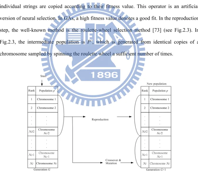
The flowchart of the learning process is shown in Fig. 2.2, where Nc is the size of population, G denote Gth generation. The learning process of the GAs involves three major steps: reproduction, crossover, and mutation. Reproduction [71]-[73] is a process in which individual strings are copied according to their fitness value. This operator is an artificial version of neural selection. In GAs, a high fitness value denotes a good fit. In the reproduction step, the well-known method is the roulette-wheel selection method [73] (see Fig.2.3). In Fig.2.3, the intermediate population is P’, which is generated from identical copies of a chromosome sampled by spinning the roulette wheel a sufficient number of times.

Figure 2.3: The roulette wheel selection.

In crossover step [74]-[78], although reproduction step directs the search toward the best existing individuals, it cannot create any new individuals. In nature, an offspring has two parents and inherits genes from both. The main operator working on the parents is the crossover operator, the operation of which occurred for a selected pair with a crossover rate. Figure 2.4 illustrates how the crossover works. Crossover produces two offspring from their parents by exchanging chromosomal genes on either side of a crossover point generated randomly.

Figure 2.4: Crossover operator.

In mutation step [79]-[85], although the reproduction and crossover would produce many new strings, they do not introduce any new information to the population at the site of an

individual. Mutation can randomly alter the allele of a gene. The operation is occurred with a mutation rate. Figure 2.5 illustrates how the mutation works. When an offspring is mutated, one of its genes selected randomly is changed to a new value.

Figure 2.5: Mutation operator.

Since GAs search many points in the space simultaneously, they have less chance to reach the local minima than single solution methods. The advantages of GAs are: 1) some individuals have a better chance to come close to the global optima solution, and 2) the genetic operators allow the GA to search optima solution. According to above reasons, GAs are suitable for searching the parameters space of neuro-fuzzy controller. For solving the problem that a neuro-fuzzy controller which performs gradient-descent based learning algorithms may reach the local minima very fast but never find the global solution, the GAs sample the parameters space of neuro-fuzzy controllers and recombine those that perform best on the control problem.

2.3 Particle Swarm Optimization

In this section, we will introduce the PSO. The standard PSO is introduced in section 2.3.1

and the CPSO is introduced in section 2.3.2.

2.3.1 Standard Particle Swarm Optimization

PSO is first introduced by Kennedy and Eberhart in 1995 [8]. It’s one of the most powerful methods for solving global optimization problems. The algorithm searches an

optimal point in a multi-dimensional space by adjusting the trajectories of its particles. The individual particle updates its position and velocity based on its previous best performance and previous best performance of other particles which denote y and respectively. A simple demonstration of how PSO learning proceeds can be shown in Fig. 2.7 as follows:

ˆy

Figure 2.6: Diagram of the PSO learning mechanism.

The position xi,d and velocity vi,d of the d-th dimension of i-th particle are updated as

follows: , ( 1) = , ( ) 1 1 ( , ( ) , ( )) 2 2 ( ( ) , ( )), ( 1) ( ) ( 1), i d i d i d i d d i d i i i v t v t c rand y t x t c rand y t x t x t x t v t + + ⋅ ⋅ − + ⋅ ⋅ − + = + + _(2.7)

where yi represents the previous best position yielding the best performance of the i-th particle;

c1 and c2 denote the acceleration constants describing the weighting of each particle been pulled toward y and y respectively; and are two random numbers in the range [0, 1].

1

rand rand₂

Let s denote the swarm size and f() denote the fitness function evaluating the performance yielded by a particle. After Eq. (2.7) is executed, the personal best position y of each particle is updated as follows:

( 1) ( 1), if ( ( 1)) ( ( )), ( 1), if ( ( 1)) ( ( )), i i i i i i i x t f x t f y y t t y t f x t f y + + ≥ ⎧ + = ⎨ _{+ + <} ⎩ t (2.8)

and the global best position is found by:

( 1) arg min ( ( 1)), 1 . (2.9)

i i

y

y t+ = f y t+ ≤ ≤i s

In 2002, Clerc [12] confirms the convergence of PSO by using a constriction factor which greatly enhances the applicability of PSO. The implementation of the constriction factor is shown in Eq. (2.10)-(2.12):

, ( 1) = [ , ( ) 1 1 ( , ( ) , ( )) 2 2 ( ( ) , ( ))], ( 1) ( ) ( 1), i d i d i d i d d i d i i i v t v t c rand y t x t c rand y t x t x t x t v t χ + + ⋅ ⋅ − + ⋅ ⋅ − + = + + (2.10) where 2 2 2 4 χ φ φ φ = − − − , (2.11) and 1 2, 4 c c φ = + φ > . (2.12) The flowchart of the PSO is shown in Fig. 2.7.

2.3.2 Cooperative Particle Swarm Optimization

The CPSO [9] is one of the most significant improvements to the original PSO. Van den Bergh presented a family of CPSOs, including CPSO-S, CPSO-SK, CPSO-H, CPSO-HK.

Algorithm CPSO-HK is the hybrid from PSO and CPSO-SK and it is proposed to address the

issue of “pseudominima.”

The concept of CPSO-S is that instead of trying to find an optimal n-dimensional vector, the vector is split into n parts so that each of n swarms optimizes a 1-D vector. The CPSO-SK

is a family of CPSO-S, where a vector is split into K parts rather than n, where . K also represents the number of swarms. Each of the K swarms acts as a PSO optimizer. The main

Figure 2.7: Flowchart of the PSO.

difference between the PSO and the CPSO is that the fitness of a single particle of the CPSO has to be evaluated through global best particles of the other swarms. Let Pj denote the j-th

swarm and Pj‧xi represents the i-th particle in the swarm j. The concept of the CPSO can be

illustrated as follows:

The fitness of Pj‧xi is defined as:

f P x( _ji _i)= f P y( ₁i …, ,P_j−1iy P x, . , ,_{j i} … P y_Ki . (2.13) ) The CPSO applies cooperative behavior to improve the PSO on find the global optimum in a high-dimensional space. This is achieved by employing multiple swarms to explore the subspaces of the search space separately to reduce the curse of dimensionality. However, there is no absolute criterion stating that the CPSO is superior to the PSO since independent changes made by different swarms on correlated variables will deteriorate its performance. In addition, in one generation of an n-dim CPSO-S operation, the computational cost is n times larger than that of a PSO operation.

2.4 Evolution Strategy with Covariance Matrix Adaptation

In this section, we introduce some background knowledge related to the proposed MS-CMA-ES. The standard CMA-ES is introduced in section 2.4.1, kernel density estimation is introduced in section 2.4.2 and mean shift procedure is introduced in section 2.4.3.

2.4.1 Standard CMA-ES

In the standard CMA-ES, a population of new search points is generated by sampling a multivariate normal distribution N with mean _m∈ n and covariance matrix _C∈ n n× _{. The}

equation of sampling new search points, for each generation number g = 0,1,2,…, reads

(g 1) ( )g ( )g _(0, ( )g _{) for 1, ,} i

x + ∼m +σ N C i= λ, (2.14) where ~ denotes the same distribution on the left and right hand side; σ(g) denotes the overall standard deviation, step-size, at generation g and λ is the sample size. The new mean m(g+1) of the search distribution is a weighted average of the μ selected points from λ samples

, ,…, ( 1) 1 g x + ( 1) 2 g x + _x(g 1) λ + :

( 1) ( 1) : 1 g i i i m w x μ λ g + + = =

∑

, (2.15) with 1 2 1 1 1, 0 i i w w w w μ = = ≥ ≥ ≥ >

∑

, (2.16)

where wi are positive weights, and x_i(_:λg+1) denotes the i-th rank individual out of λ samples. The index i:λ denotes the i-th rank individual and

, (2.17) ( 1) ( 1) ( 1) 1: 2: : ( g ) ( g ) ( f x_λ+ _≤ f x _λ+ _{≤ ≤} f xg ₎ λ λ+

where f(‧) is the objective function to be minimized. The adaptation of new covariance

matrix C(g+1) is formed by a combination of rank-μ and rank-one update [13]

(

)

(

( 1) ( ) cov ( 1) ( 1) ( 1) ( 1)

cov cov : :

1

cov cov

rank-one update _{rank- update}

1 (1 ) (1 ) T T g g g g g c c i i i i c c p p c w y y μ λ λ μ μ μ + + + = = − + + − ×

∑

C C + g+

)

_{, (2.18)}

where μcov ≥ 1 is the weighting between rank-μ update and rank-one update; ccov∈[0,1] is the learning rate for the covariance matrix update, and

( 1) ( 1) ( ) ( )

: ( : ) /

g g g i i

y _λ+ ₌ x_λ+ ₋m _σ g _(2.19)

is a modified formula used to compute the estimated covariance matrix for the selected samples. The evolution path (g 1) for rank-one update is described as follows:

c p + ( 1) ( ) ( 1) ( ) eff ( ) (1 ) (2 ) g g g g c c c c c g m m p c p c c μ σ + + _{= − + −} − _{, (2.20)}

where cc ≤ 1 denotes the backward time horizon and 1 2 eff 1 i i w μ μ − = ⎛ ⎞ = ⎜ ⎝

∑

⎠⎟ (2.21) denotes the variance effective selection mass. The new step-size σ(g+1) is updated according to

( 1) ( 1) ( )_{exp 1} (0, ) g g g c p d E N σ σ σ σ σ + + ₌ ⎛_⎜ ⎛_⎜ ⎞⎞ ⎜ ⎜ _{⎝ ⎠}⎟ ⎝ I ⎠ ⎟ ⎟ − ⎟ , (2.22) with

1 2 ( 1) ( ) ( 1) ( ) ( ) eff ( ) (1 ) (2 ) g g g g g g m m p_σ c p_{σ σ} c_σ c_σ μ σ − + + _{= − + − C} − _{, (2.23)}

where cσ is the backward time horizon of evolution path, similar to cc; dσ is a damping

parameter and _p(g 1)

σ + is the conjugate evolution path for step-size σ(g+1). The expectation of the Euclidean norm of a N(0, I) reads

1

(0, ) 2 ( ) / ( ) (1/ )

2 2

n n

E N I = Γ + Γ ≈ n O+ n . (2.24) where Γ() denotes the gamma function and O() represents high-order terms.

2.4.2 Kernel Density Estimation

In parametric model estimation analysis, we need to suppose the distribution of data points coincides with certain model. Empirical evidence have shown that there tends to exist large differences between parametric estimation-based models and real-world physical models. Based on above defects, Rosenblatt and Parzen proposed a non-parametric way called kernel density estimator [66] to estimate the unknown p.d.f. of a random variable. The kernel density estimator does not require prior knowledge of how data distribute; instead, it analyzes the characteristic of the distribution of data. Hence, it is highly valuable in both statistical theory and application.

In the proposed MS-CMA-ES, sampled search points in the search space are considered as data in the feature space. It is very intuitive since the location of search points tends to be the phenomenal feature in function optimization problems. The rationale behind density estimation-based clustering approach is that the feature space can be regarded as the empirical p.d.f. Due to the fact that search points are sampled from normal distribution with adjusted mean and adapted covariance matrix, and are further selected according to their fitness, dense regions in the search space correspond to local maxima of the p.d.f.; in other words, the modes of the unknown density. Consider n points xi, i = 1,…, n, in the d-dimensional space

definite matrix bandwidth matrix H, computed in the point x is given by 1 1 ˆ ( )_h n _h( ) i i f x K x n = x =

∑

− , (2.25) with 1 ( ) ( ) h x K x h K h − = , (2.26) where Kh(x) is a d-variate kernel function satisfying

( ) 1 h K x dx ∞ −∞ =

∫

. (2.27)

Normally speaking, kernel functions are symmetric, unimodal probability density functions. Uniform, normal and Epanechnikov kernel are the most common seen. It has been proven that, in certain routine conditions, kernel density estimator approximates the real density functions gradually with increasing sampling size [86]. Although the choice of different kernel functions have different effects on the results, but the effect appears small compared with the effect caused by the bandwidth, so researches focus more on the selection of bandwidth [87]. Theoretically, the selection of bandwidth is based on the mean integrated square error (MISE) between kernel density estimation and the real density function. However, the computation of MISE is too complicated. In practice, how selection of bandwidth affects the performance is analyzed by computing an asymptotic mean integrated error (AMISE) from a large number of samples. Recently, many literatures use plug-in method and cross-validation method to determine the optimal bandwidth, so that the selection of bandwidth no longer depends on the prior guess of true density function [86, 87]. In addition to the aforementioned fixed bandwidth mechanism, the variable bandwidth mechanism, bandwidth varies with different sample position, is also widely adopted in practice [88, 89]. Because it is very difficult for the fixed bandwidth mechanism to properly address multimodal density functions, especially in cases when density of each peak varies greatly. However, the analysis is relatively more complicated when compared with fixed bandwidth mechanism. In practice, the utilization of variable bandwidth mechanism is mostly based on rule of thumb [86]. If the variable

bandwidth mechanism is adopted, the kernel density estimator Eq. (2.25) becomes 1 1 ˆ ( ) n ( _i) i f x K x n = =

∑

− H H x , (2.28) where 1/ 2 _{1/ 2} ( ) ( ) K x ₌ − K − x H H H , (2.29)

H is the symmetric, positive definite bandwidth matrix.

2.4.3 Mean Shift Procedure

Mean shift procedure is a very versatile tool for feature space analysis and it is applicable to many field of tasks [90-92]. In the previous research [65], authors successfully extend this algorithm to computer vision applications, and have attracted huge attention. Mean shift procedure is an iterative algorithm based on kernel density estimation, which continually updates the mean shift vectors of data points according to the gradient of kernel function. Although the mean shift algorithm is very simple in form, but in practice there is a high efficiency and stability. The most classic application is the mean shift-based clustering algorithm. If we can have a good estimation of bandwidth, mean shift-based clustering algorithm would be a nice alternative relative to algorithms that the number of clusters needs to be pre-set, such as K-means algorithm. In the proposed MS-CMA-ES, search points in the search space are considered as data in the feature space. It is very intuitive since location of search points tends to be the phenomenal feature in function optimization problems. Due to the fact that, in the MS-CMA-ES, sampled search points are further selected according to their fitness, dense regions in the search space correspond to local maxima of the p.d.f.; in other words, the modes of the unknown density.

Consider the density estimation kernel Kh(x) introduced earlier this section. If the profile

notation [21] is employed, the kernel Kh(x) can also be written as 2

where kh(x) is a radially symmetric kernel defined as the profile of the Kh(x), and ck,d is the

normalization constant which makes Kh(x) integrate to one. If we define

( )g x_h = −k x_h′( ), (2.31) the d-variate kernel Gh(x) can also be written as

2 ,

( ) ( )

h g d h

G x =c g x , (2.32) and similarly, cg,d denotes the normalization constant. The density estimation kernel Kh(x) is

also called the shadow kernel of Gh(x) [65]. Consider n points xi, i=1,…, n, in the

d-dimensional space d, the mean shift vector at x is given by

1 1 ( ) ( ) ( ) n i h i i n h i i x G x x m x x G x x = = − = − −

∑

∑

. (2.33)

Intrinsically, mean shift procedure can be viewed as a mode seeking method [59], which determines the modes of p.d.f. estimated by kernel Kh(x). Denote {yj}j=1,2,… the sequence of

successive search locations of kernel Gh, from Eq. (2.33) it has the form

1 1 1 ( ) 1, 2, ( ) n i h j i i j n h j i i x G y x y G y x = + = − = −

∑

∑

j= (2.34)

and y1 is the initial search location. The corresponding sequence of density estimates computed with kernel Kh is given by

{

fˆh K, ( )j

}

= f yˆh( ) j j=1, 2, . (2.35)

In the previous research [59], authors have proven that once search location yj gets sufficiently

close to a mode of estimated density function fˆ_{h K,} , it converges to it, and the set of all locations converge to the same mode is defined as the basin of attraction of that mode. The general steps of applying mean shift procedure is listed as follows:

Step 2: Sequentially or parallelly run the mean shift procedure until the search points converge.

Step 3: Each convergence point defines a mode and each initial location converges to that mode defines the basin of attraction of that mode.

CHAPTER 3

EVOLUTIONARY ALGORITHMS

In this chapter, the proposed four algorithms are discussed. In section 3.1, a Q-valued based particle swarm optimization and the concept of using Lyapunov design principles for constructing safe reinforcement learning agents are introduced. In section 3.2, the proposed two-strategy reinforcement (TSR) learning mechanism and the group-based symbiotic evolution (GSE) which enables the learning agent to evaluate the fuzzy rule locally are introduced. In section 3.3, a separability detection approach to cooperative particle swarm optimization (SD-CPSO) for placing correlated variables into the same swarm is discussed. In section, 3.4, the proposed mean shift based evolutionary strategy with covariance matrix adaptation (MS-CMA-ES) is introduced. We cannot directly apply mean shift clustering to the sampled points generated by CMA-ES because the adopted mean shift clustering requires independent identity distribution of samples to perform density estimations. Several previous works such as importance sampling [93,94] and bandwidth estimation [86,87] are also discussed in this section.

3.1 Q-value based PSO

Thorough learning algorithm of QPSO is described in this section. The architecture is shown in Fig. 3.1. The whole learning process can be roughly divided into two parts: the Q-value and PSO operation part. The learning strategy for Q-values of particles is detailed in section 3.1.1 while the PSO operation and the flowchart of QPSO are described in section 3.1.2.

Figure 3.1: Architecture of QPSO.

3.1.1 Learning Q-values of Particles

In QPSO learning, if there are s particles in the swarm, s trials are taken in one generation. The agent applies in each trial an action to the environment by selecting a particle based on its Q-value. Every time a particle is selected, the Q-value of the selected particle is updated based on the system’s reward. If the -th particle is selected, its Q-value qi i is updated as

* 1 ( ) ( ) [ ( ( 1)) ( )] i i i q t q t Q x t q t t α γ = + − + + − , (3.1)

for i=1…s, where

* * ' ( ( 1)) 1... 1... ( ( 1)) max ( ( 1), ') max ( ( 1), ) max ( ) ( ). a A x t i i s i i i s Q x t Q x t a Q x t p q t q t ∈ + = = + = + = + = = (3.2) That is * 1 ( ) ( ) [ ( ) ( )] ( ) ( ), i i i i i i q t q t q t q t t q t t α γ αδ = + − + − = + (3.3) for i=1, ,s, where δ_i( ) t is regarded as TD error.

fitness values for PSO evolution.

3.2.2 Q-value based PSO

The PSO operation used in QPSO consists of two major steps: swarm initialization and Q-valued base PSO evolution. Details of these two steps are described step-by step as follows. ‧ Swarm initialization:

The particle swarm is composed of particles encoded by the parameters on a NFS. Each particle is encoded by the mean, deviation of Gaussian membership functions and the weightings for output action strength. The number of fuzzy rules determines the length of each particle. After the number of rules is set, the initial particles are generated according to the following equations:

[ ]

[

min max

]

Mean: x , , where 1, 3, , 2 -1; 1, 2, , . i n random m m n NR i = = = s (3.4)

[ ]

[

min max

]

Deviation: x , , where 2, 4, , 2 . i n random n NR σ σ = = (3.5)

[ ]

[

min max

]

Weight: , , where 2 1, 2 2, , . i x n random w w n NR NR D = = + + (3.6) i

p represents the i-th particle in the swarm; N represents the input dimension; R

represents the number of fuzzy rules; D represents the size of each particle, usually D

equals to (N+1)R in most of cases where the dimension of output variable is 1;

[

mmin,mmax

]

,

[

σmin,σmax

]

and

[

wmin,wmax

]

are the predefined ranges. The above

equations result in the coding scheme between a neural fuzzy system and a particle shown in Fig. 3.2.

Figure 3.2: Coding scheme between a particle and a TSK-type NFS in QPSO.

‧ Q-value based PSO evolution:

The Q-values derived in Eq. (3.3) are used as the fitness values for PSO evolution. The Q-value of each particle determines the performance of a particle for controlling the system. In the proposed QPSO, the Q-value of each particle indicates how soon a particle can guide the system’s state to reach the set of goal states. The learning processes proceed to new generation until a predefined stop criterion is met. The block diagram of whole learning process in QPSO is shown in Fig. 3.3.

3.2 Two-strategy Reinforcement Evolutionary Algorithm

The proposed two-strategy reinforcement evolutionary algorithm (TSR-EA) is introduced in this section. Two major modifications are proposed in this algorithm: a two-strategy

reinforcement signal design and the group-based symbiotic evolution (GSE). Details of these two operations are described as follows:

3.2.1 Two-strategy Reinforcement Signal Design

The TSR-EA is constructed on a TSK-type NFS model. The NFS model acts as a control network to determine a proper action according to the current input vector (environment state). The feedback signal is the reinforcement fitness value that functions as a performance measurement. The reinforcement learning architecture adopted in the TSR-EA is the time-step reinforcement architecture [95]-[97]. In this architecture, the only available feedback is a reinforcement signal that notifies the model only when a failure occurs. This architecture is straightforward and easy to implement. However, its fitness function can only indicates how long can the controller work well instead of measuring how soon the system can enter the desired state, which is also very important. Most reinforcement learning algorithms offer no guarantee on stabilizing a system around a certain operating point, or keeping the state of a system within a certain range. In this dissertation, the proposed QPSO described in section 3.1 can meet the aforementioned goals by adopting the concept of safe reinforcement learning agents based on Lyapunov design principles proposed Perkins and Barto [57]. Using the concept proposed in [57], the QPSO can guide the state of a system to reach and remain in a desired set of goal states by constraining the action choices of the agents. Actions constrained by Lyapunov design principles cause the system to descend on an appropriate Lyapunov function. The feedback reinforcement signal of in the QPSO is the time step that indicates how soon the system enters the desired set of goal states. The QPSO provides not only

reliable initial learning performance but also accurate learning result. However, in order to apply Lyapunov design principles, we have to identify the Lyapunov function of a control plant in advance, which refers to the requirement of more information about the state of the control plant. For some real-world applications, some states are difficult or expensive to obtain. As a result, in the TSR-EA method, we proposed the TSR design so that our method can enjoy the convenience brought by the standard reinforcement learning architecture on one hand, and the accurate learning performance on the other. The TSR learning signal design for determining the fitness value of each learning trial is described as follows.

The proposed two strategies are judgment and evaluation. The judgment strategy measures the fitness value of a learning trial that fails to maintain the system’s state in a desired operating range, whereas the evaluation strategy measures the fitness value of a learning trial that works the system well in the original successful range, but fails under a stricter successful range is applied. At first, for each different control task, a corresponding operating range Original_Range is predefined. Then, we shrink the original successful operating range as the control time step increases, as defined in Eq. (3.7).

(

)

(

)

_ = _ , where 1, if , _ _{, if < _ ,} _ , , _

Strict Range Original Range

t A

Thres TimeStep A t _{A t Thres TimeStep}

Thres TimeStep A _otherwise Thres TimeStep δ δ × ⎧ ⎪ ≤ ⎪⎪ + − =_⎨ ≤ ⎪ ⎪ ⎪⎩ (3.7)

where A is a parameter that simply prevents the modified range from becoming zero. This equation provides guidance to the controller to meet the control goal sooner. The

Original_Range and Strict_Range are both considered as stopping criteria. If a learning trial

fails because the system state falls beyond the Original_Range, this learning trial is then considered as failing under a “looser” constraint. Hence, a smaller fitness value is obtained from this learning trial. On the contrary, if a learning trial fails for the system state deviating