即時車輛導航系統之GPS/INS/GIS整合設計

全文

(1)國立交通大學電機與控制工程學系碩士論文. 即時車輛導航系統之 GPS/INS/GIS 整合設計 Design of GPS/INS/GIS for a Real-Time Vehicle Navigation System. 研究生：楊世宏指導教授：陳永平. 教授. 中華民國九十三年六月.

(2) 即時車輛導航系統之 GPS/INS/GIS 整合設計. Design of GPS/INS/GIS for a Real-Time Vehicle Navigation System 研究生：楊世宏. Student：Shih-Hung Yang. 指導教授：陳永平教授. Advisor：Professor Yon-Ping Chen. 國立交通大學電機與控制工程學系碩士論文. A Thesis Submitted to Department of Electrical and Control Engineering College of Electrical Engineering and Computer Science National Chiao Tung University In Partial Fulfillment of the Requirements For the degree of Master In Electrical and Control Engineering June 2004 Hsinchu, Taiwan, Republic of China. 中華民國九十三年六月.

(3) 即時車輛導航系統之 GPS/INS/GIS 整合設計. 學生：楊世宏. 指導教授：陳永平教授. 國立交通大學電機與控制工程學系. 摘要本論文提出一套以卡爾曼濾波器整合全球定位系統與慣性導航系統的即時車輛導航系統，再利用地圖匹配演算法消除來自卡爾曼濾波器的誤差，且找到正確的道路與位置。此硬體架構整合一個加速規與一個陀螺儀量測二維位移、速度、車頭方向，同時設計了兩個微算器以擷取全球定位系統接收器與慣性量測元件之資料，然後傳送到主處理器運算。接著主處理器利用卡爾曼濾波器來估算最佳導航資訊。此外本論文提出一個修正的地圖匹配演算法以調整車頭方向。最後最佳導航資訊將會顯示在使用者之圖示介面。實驗結果將證實提出的方法對於車輛行經都市區、地下道、樹林茂盛的地區時是有效且可實現的。. i.

(4) Design of Integrated GPS/GIS for a Real-Time Vehicle Navigation System. Student: Shih-Hung Yang. Advisor: Professor Yon-Ping Chen. Department of Electrical and Control Engineering National Chiao Tung University. ABSTRACT In this thesis, a GPS/INS navigation system integrated by Kalman Filter is proposed. Furthermore, a map-matching algorithm that eliminates the error of GPS/INS and finds the correct road and position on the map is also applied to this real-time vehicle navigation system. One accelerometer and one gyro are integrated in the system to obtain 2-D displacement, velocity, and heading direction. Two microprocessors are designed to capture both the signals of GPS receiver and IMU set, and then transmit data to the main processor. After that, the optimal navigation information of GPS/INS is estimated in the main processor by the Kalman filter. In addition, a modified map-matching algorithm is adopted to adjust the heading direction of vehicle. Finally, the optimal navigation information would be shown in a graphical user interface. The experiment results would demonstrate the effectiveness and applicability of the proposed methods as the vehicle runs in the urban area, underground passage, and wooded area. ii.

(5) Acknowledgment 在兩年的研究過程中，首先要感謝我的指導老師陳永平教授，教導我們正確的研究方法、態度以及解決問題的能力，在研究同時，也親自批改我們的論文，增長我們英文寫作能力，此外，也感謝忠隆、佳宏學長，儘管畢業在外工作，也不時幫助我的研究，在實驗上，更要感謝翰宏同學開車進行實驗，成果才會如此完美。研究所兩年中，很感謝室友智傑的鼓勵，不管在學業、研究、生活，都能彼此互相鼓勵、扶持，也謝謝實驗室的伙伴，尤其是一起畢業的翰宏、依娜、智淵、倉鴻、培瑄，生活中有了你們的陪伴，才能如此快樂，還有手語 91 的同伴們，彼此關懷近況，也謝謝 Campus 的鼓舞以及生活上的支持，這本論文富含著你們的色彩，最後，我要感謝我的家人，給予無時無刻的照顧。僅以此篇獻給所有關心、照顧我的朋友們。楊世宏 2004/7/6. iii.

(6) Contents. Chinese Abstract. i. English Abstract. ii. Acknowledgement. iii. Contents. iv. Index of Figures. vi. Index of Tables. viii. Chapter 1 Introduction. 1. Chapter 2 Global Positioning System. 3. 2.1 Introduction. 3. 2.2 GPS Satellite Signals. 4. 2.3 GPS Navigation Message. 6. 2.4 GPS Observations. 7. 2.4.1 Pseudo Range. 7. 2.4.2 Carrier Phase. 8. 2.5 GPS Error Sources. 8. 2.6 Position Accuracy and DOP. 9. 2.7 Differential GPS Technique. 10. 2.8 The Positioning Equation. 11. Chapter 3 Inertial Navigation System 3.1 System Overview. 13 13. 3.1.1 Gimballed System. 13. 3.1.2 Strapdown System. 14. 3.2 Coordinate Frames and Transformation. 15. 3.2.1 Coordinate Frames. 15. 3.2.2 Transformation Between ECEF and Geodetic Frames. 17. 3.2.3 Transformation Between Body And Navigation Frames. 19. 3.3 Dynamic Equations In Navigation. 21. 3.3.1 Coordinate Transformation Matrix Properties iv. 21.

(7) 3.3.2 Velocity Dynamic Equation. 23. 3.4 INS Error Model. 27. 3.4.1 Error Model. 27. 3.4.2 Error Sources. 29. 3.4.3 The Reduced Error Model. 33. Chapter 4 Geographic Information System. 34. 4.1 Introduction. 34. 4.2 Reference Ellipsoids and Projection. 34. 4.3 Taiwan Coordinates. 37. 4.4 Map-Matching Algorithm. 38. 4.4.1 Map Matching Issues. 38. 4.4.2 Map Matching Structure. 40. 4.4.3 Initial Mode. 41. 4.4.4 Node Nearby Detection and Searching Mode. 41. 4.4.5 Tracking Mode. 44. Chapter 5 Integration of GPS/INS/GIS. 45. 5.1 Motivation. 45. 5.2 Integration Mode. 46. 5.3 Filter Design. 50. 5.3.1 Discrete Linear Dynamics Model and Observation Model. 50. 5.3.2 Optimal State Vector Estimation. 52. 5.4 Navigation System Design. 54. 5.4.1 Hardware and Software. 54. 5.4.2 Programming Procedure. 56. 5.5 Experiments. 61. Chapter 6 Conclusions. 67. References. 70. v.

(8) List of Figures Figure 2.1 Global Positioning System Overview. 3. Figure 2.2 GPS Satellite Signals. 5. Figure 2.3 GPS Navigation Data Format. 6. Figure 2.4 Dilution of Precision. 10. Figure 2.5 Differential GPS Technique. 11. Figure 2.6 GPS Positioning Method. 12. Figure 3.1 The gimballed INS system. 14. Figure 3.2 Body (Vehicle) coordinate frame. 15. Figure 3.3 Navigation frame or tangent plane reference coordinate frame. 16. Figure 3.4 ECEF rectangular coordinate system. 16. Figure 3.5 Geodetic reference coordinate system. 17. Figure 3.6 Relation between body and navigation frame. 19. Figure 3.7 Rotation by the Euler angles. 20. Figure 3.8 Gravitational acceleration vector in the navigation frame. 25. Figure 4.1 Semi-major axis and semi-minor axis. 35. Figure 4.2 Projections and the appearance of the Graticules. 36. Figure 4.3 Azimuthal projection. 36. Figure 4.4 Projected errors. 39. Figure 4.5 Dot-product. 39. Figure 4.6 Moving distance. 39. Figure 4.7 Map matching flowchart. 40. Figure 4.8 Initial mode. 41. Figure 4.9 Searching mode flowchart. 42. Figure 4.10 Condition 2. 43 vi.

(9) Figure 4.11 Tracking mode. 44. Figure 5.1 GPS/INS integration scheme. 46. Figure 5.2 GPS/INS without GIS fix. 47. Figure 5.3 GIS fix GPS/INS. 48. Figure 5.4 Turn Detect Range. 48. Figure 5.5 GIS fix GPS/INS. 49. Figure 5.6 GPS/INS/GIS integration mode. 49. Figure 5.7 Raw Map Data Format. 55. Figure 5.8 Shapefile in ArcView. 56. Figure 5.9 The data flowchart in two microprocessors. 57. Figure 5.10 Heading direction estimation. 59. Figure 5.11 Initialize heading direction for INS. 59. Figure 5.12 Check position reliability. 60. Figure 5.13 Path 1. 62. Figure 5.14 Path 2. 62. Figure 5.15 Path 1 result without GIS correction. 63. Figure 5.16 Path 1 result with GIS correction. 65. Figure 5.17 Path 2 result. 66. Figure 5.18 Experiment equipment. 66. vii.

(10) List of Tables Table 2.1 User equivalent range error (UERE). 11. Table 4.1 Ellipsoidal Parameters. 35. Table 4.2 Selected reference ellipsoids. 35. Table 4.3 Taiwan coordinates. 37. viii.

(11) Chapter 1. Introduction. In recent years, many research are devoted to the real-time car navigation systems. Some of them are concentrated on position estimation; some developed systems gave the shortest route. They are all expected to communicate with traffic management in the future. The car navigation system mainly provides the position estimation. Dead reckoning and Inertial Navigation System (INS) has been adopted to estimate vehicle’ s position. They estimate position from integrating the displacement, acceleration, and angular rate at every sampling time. However, this estimated method would produce large error due to the fact that the error would be accumulated from surface roughness or sensor error for a long time. To remedy this problem, the Global Positioning System (GPS) attractive in car navigation system is employed to provide the absolute position every second if more than four satellites were observed. However, the GPS is subject to the signal outage, interference, and jamming. On the contrary, INS is a self-contained and much immune to surrounding environment. The best way to obtain the optimal position estimation is to combine GPS and INS. In order to combine them, most researchers relied on Kalman filter, which is a recursive algorithm and requires external measurements to compute optimal corrections of system state variables. The assumptions in the use of Kalman filter are the system is linear and the noise is white Gaussian. However, the system model in INS is nonlinear and the noises of GPS and INS aren’ t Gaussian. The position estimation from Kalman filter is not optimal. The map-matching algorithm is a useful method to eliminate the error according to the exact position in map, as reliable road maps are available. The map-matching algorithm is a scheme to find the road and position where the vehicle runs. The fact is. 1.

(12) that the vehicle always runs on the road and the error from filter would be eliminate if the position of vehicle is known in the road on map. [11] However, this algorithm would leads to mapping error as the GPS signal is unavailable and the error accumulation from INS is too large. In this thesis, a modified map-matching algorithm is proposed to solve this problem. This modified algorithm, heading direction estimation, employs the direction of road to adjust the heading direction of vehicle. Furthermore, as the vehicle makes a turn, the INS would measure the variation of angular rate and the GIS would detect if there were a node near the vehicle. There are some roads that are new built and don’ t updated in the GIS database. The proposed method would detect whether there were a road near the vehicle or not. If not, that means the GIS is fail, the GPS/INS trajectory would replace the matching point from GIS. The practical experiment would show the effectiveness and applicability of the proposed algorithm. In chapter 2, the Global Positioning System (GPS) is presented to introduce how the GPS determine the absolute position. The chapter 3 will discuss the Inertial Navigation System (INS) and present the dynamic equation and error model in INS. In chapter 4, the geographic information system (GIS) is introduced to know the Taiwan coordinates and the map-matching algorithm. The chapter 5 will present the integration of GPS/INS/GIS and the proposed method, heading direction estimation, is provided. The real road experiment results are also shown in this chapter. Concluding remarks are given in chapter 6.. 2.

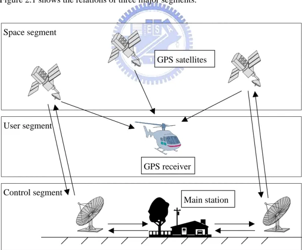
(13) Chapter 2. Global Positioning System. 2.1 Introduction NAVSTAR GPS, an acronym standing for Navigation System with Timing and Ranging Global Positioning System, is designed to provide highly accurate, 24-hour and worldwide coverage for position reporting and created by the United States Department of Defense. The NAVSTAR GPS consists of three major segments: A. The space segment B. The user segment C. The control segment Figure 2.1 shows the relations of three major segments.. Space segment GPS satellites. User segment. GPS receiver Control segment. Main station. Figure 2.1 Global Positioning System Overview [23]. 3.

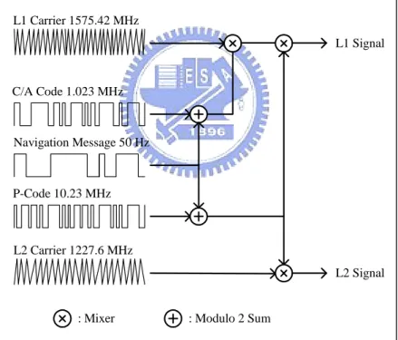
(14) The space segment of the GPS includes 21 working satellites and 3 spares, and they are arranged in six nearly circular orbit planes, which contain four satellites each plane. The 24 spacecraft are placed in 20,200 km circular orbits inclined at 55 degrees and surround Earth with approximately 12 sidereal hours. The control segment is made up of a master control station, worldwide monitor stations and ground control stations. These monitor stations track the satellites continuously all day, and they measure signals from the space vehicles (SVs), which are incorporated into orbital models for each satellite. The models compute precise orbital data (ephemeris) and SV clock data to the SVs. Then the SVs send subsets of the orbital ephemeris data to GPS receivers. Thus, the purpose of the control segment is to track the GPS satellites and correct ephemeris constants and clock-bias errors. The user segment consists of the GPS receivers and the user community. As GPS receivers receive four satellites signals, the four dimensions, x, y, z, and time would be calculated from triangulation. The receiver measures the pseudo range and carrier phase from the satellite. Furthermore, the satellites provide two different accurate signals. Coarse-Acquisition Code (C/A) is used for civilian and Precision Code (P) provides more accurate positional precision.. 2.2 GPS Satellite Signals Each satellite transmits a unique coded signal that consists of the identification of the satellite and the ranges to it. The satellite signals based on two L-band frequencies centered on 1575.42 MHz (L1 frequency) and 1227.60 MHz (L2 frequency), which are derived from a fundamental clock frequency of 10.23 MHz. The L1 frequency carries the navigation message and the Standard Positioning Service (SPS) code signals. The L2 frequency is used to measure the ionospheric delay by Precise 4.

(15) Positioning Service (PPS) equipped receivers. The C/A Code, which modulates the L1 carrier phase, is a repeating 1 MHz Pseudo Random Noise (PRN) code. This noise-like code modulates the L1 carrier signal to spreading the spectrum over 1 MHz bandwidth. Each SV has different C/A code PRN, i.e. satellites are identified with their PRN number. The P-Code, is a 10 MHz PRN code, modulates both the L1 and L2 carrier phases. In the Anti-Spoofing (AS) mode of operation, the P-Code is encrypted into the Y-Code that is used by authorized users with cryptographic keys. Therefore, the C/A Code and P (Y)-Code are the basis of civil SPS and PPS respectively. Figure 2.2 schemes the structure of GPS satellite signals. L1 Carrier 1575.42 MHz L1 Signal. C/A Code 1.023 MHz. Navigation Message 50 Hz. P-Code 10.23 MHz. L2 Carrier 1227.6 MHz L2 Signal. : Mixer. : Modulo 2 Sum. Figure 2.2 GPS Satellite Signals. 5.

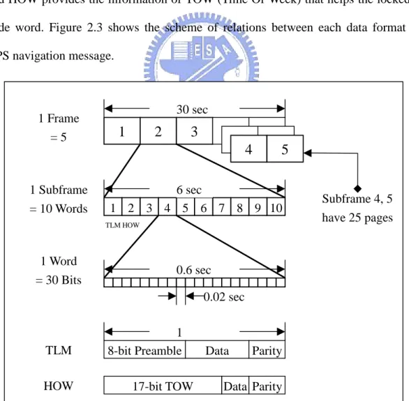
(16) 2.3 GPS Navigation Message GPS navigation message, a 50 Hz signal, consists of data bits that describe the GPS satellite orbits, clock corrections, and other system parameters. A data bit frame, which is transmitted every 30 seconds, consists of 1500 bits divided into five 300-bit subframes. The subframes 1, 2, and 3 contain orbital and clock data where subframe 1 send SV clock corrections and subframes 2 and 3 send precise SV orbital data sets (ephemeris data parameters). Furthermore, subframes 4 and 5 transmit different pages of system data. In addition, each subframe comprises the telemetry word (TLW) and the handover word (HOW). TLW tells the receiver what the subframe data received, and HOW provides the information of TOW (Time Of Week) that helps the locked P code word. Figure 2.3 shows the scheme of relations between each data format in GPS navigation message.. 1 Frame =5. 30 sec. 1. 2. 3 4. 1 Subframe = 10 Words. 5. 6 sec 1 2 3 4 5 6 7 8 9 10 TLM HOW. 1 Word = 30 Bits. 0.6 sec 0.02 sec. TLM HOW. 1 8-bit Preamble. Data. 17-bit TOW. Parity. Data Parity. Figure 2.3 GPS Navigation Data Format 6. Subframe 4, 5 have 25 pages.

(17) 2.4 GPS Observations There are two fundamental observations, pseudo range and carrier phase, which can determine the user location. In general, the pseudo range, the main positioning tool, is utilized with less computation, and the carrier phase is always used in high precision surveying that costs a lot of time to obtain the high precision position. The two observations would be presented in the following sections.. 2.4.1 Pseudo Range The pseudo range measures the distance by decoding the P or C/A code at the epochs between transmitting and receiving the signals. In fact, because the clock of the satellites and the receivers are asynchronous, this method is not achievable and timing errors might be cause. Not only the asynchronous effect, but the tropospheric and ionospheric propagation delays also affect the measurement of pseudo range. Thus, the general expression of pseudo range can be interpreted as: [23] PR R c   t r t s  c  t a. (2.4.1). where PR : Pseudo range R : True range. c : Light speed. t r : Receiver clock bias t s : Satellite clock bias t a : Atmospheric propagation delay. 7.

(18) 2.4.2 Carrier Phase Carrier phase tracking GPS signals requires specially equipped carrier tracking receivers and has a revolution in land surveying. L1 and L2 cycles have wavelengths of 19 and 24 centimeters respectively. These carrier signals can provide ranging measurements with around millimeters accuracy under special circumstances. However, it always costs much time to get high precision position, and therefore the carrier phase is generally used in surveying. The carrier phase observation is still affected from the receiver clock error and the atmospheric propagation. Furthermore, as using carrier phase observation, there would be two problems, which affect the positioning accuracy. One is the cycle or phase ambiguity problem, and the other is the cycle slips problem. With the description above, the general expression of the carrier phase observation equation can be shown as: [23] f   R c t r t a t s  N  c. (2.4.2). where.  : Carrier phase observation. f : Carrier wave frequency. N : Cycle ambiguity..  : Other noise.. 2.5 GPS Error Sources The accuracy of GPS position measurements depends on the quality of the pseudo range measurements and satellite ephemeris data. The major error factors that 8.

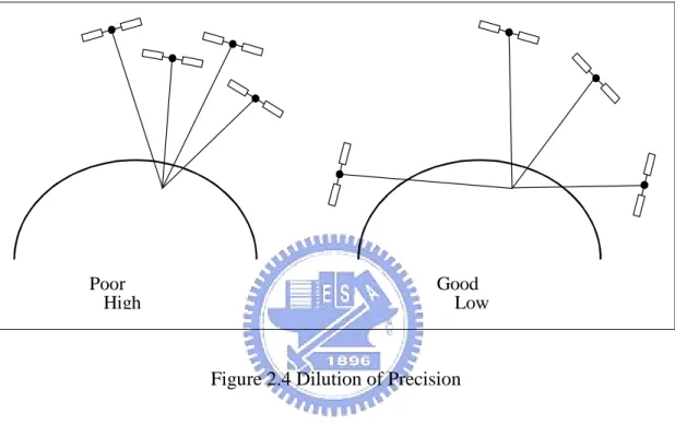
(19) affect the accuracy of the GPS measurements are: [24] A. Satellite clock errors B. Ephemeris errors (satellite position errors) C. Receiver errors D. Ionosphere errors (upper atmosphere errors) E. Troposphere errors (lower atmosphere errors) F. Multipath errors (errors from bounced signals) G. Selective Availability errors The main GPS error source is the Selective Availability errors that are the signal transmission perturbations and produced by the NAVSTAR managers. However, the SA errors were removed at May 20, 2000, and therefore the GPS positioning accuracy can be up to 10~20 m level now.. 2.6 Position Accuracy and DOP [24] Dilution of Precision (DOP) is a value, which is the exception quality of position measurement based solely on the geometric arrangement of the satellites and the receiver being used for the measurement. When DOP value is unity, the accuracy is as good as it can be considering all the sources of error. This might occur when one satellite is overhand and the three others located in the horizon with 120 degrees to each other. Figure 2.4 shows the scheme of DOP. The overall DOP number includes several sub-DOPs: A. HDOP (Horizontal DOP) is a combination of NDOP (North DOP) and EDOP (Earth DOP). 9.

(20) B. VDOP (Vertical DOP). C. PDOP (Position DOP) is a combination of HDOP and VDOP. D. TDOP (Time DOP). E. GDOP (Geometric DOP) is a combination of PDOP and TDOP.. Poor High. Good Low. Figure 2.4 Dilution of Precision. 2.7 Differential GPS Technique All receivers in the same local geographic area have similar qualities of errors outlined in the section 2.5. Thus, the Differential GPS (DGPS) employs this characteristic and attempts to compensate the other receivers with a base station, whose accurate position is know, situated at a precisely surveyed location. This base station, like all other receivers, obtains signals and errors from the satellites and determines the range errors by differencing the calculated and the measured ranges. Then, these errors are broadcast to other receivers in the same local geographic area, so that the range measurements of receivers can be corrected and the more accurate position estimate can be also obtained. [23] Figure 2.5 shows that the reference station. 10.

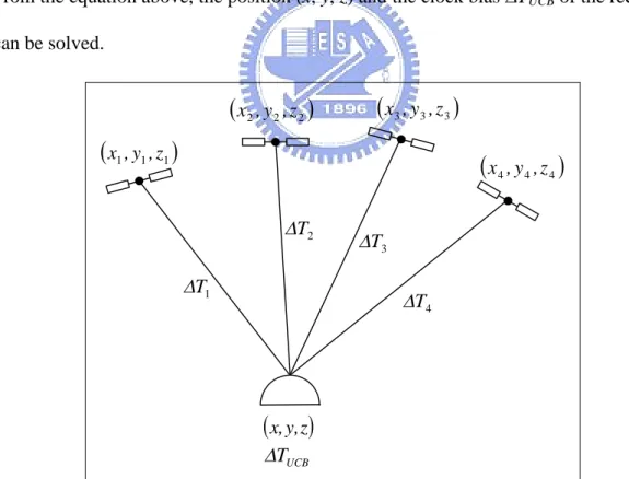
(21) receives and calculates the errors, and then transmits errors to the other receivers to correct the position error. Table 2.1 shows the set of error sources between GPS and DGPS. It is clear that DGPS is more accurate than GPS.. Reference Station. GPS Receiver Correction Processor. Figure 2.5 Differential GPS Technique Table 2.1 User equivalent range error (UERE) [11] Predicted Error (m) Error Sources Satellite ephemeris error Satellite clock error Multipath error Ionosphere error Troposphere error Receiver error User ranging error (RMS). P code 2.62 3.48 1.22 0.4 0.4 0.24 4.25. GPS C/A code 2.62 3.48 3.48 6.4 0.4 2.45 8.54. P code 0 0 1.22 0.15 0.15 0.24 1.28. DGPS C/A code 0 0 3.48 0.15 0.6 2.45 3.96. 2.8 The Positioning Equation This section would present how to determine the coordinate and time from observing four satellites. When the satellites are observed, each satellite signal can provide its position (xi, yi, zi) and the PRN code time Ti shown as figure 2.6. The 11.

(22) position (x, y, z) and the clock bias TUCB of the receiver can be solved by using the signal provided from each observed satellite. Thus, the basic observable equation can be shown as follows: [10] Ri c  Ti TUCB   xi x  yi y  z i z  i 1,2,3,4 2. 2. 2. (2.8.1). where Ri : Pseudo range between receiver and the ith observable satellite.. c : Light speed.. Ti : PRN code delay time.. xi , yi , zi : Position of the ith observable satellite. From the equation above, the position (x, y, z) and the clock bias TUCB of the receiver can be solved.. x 2 , y 2 , z 2 . x3 , y3 , z 3 . x1 , y1 , z1 . x 4 , y 4 , z 4  T2. T3. T1. T4. x, y, z TUCB Figure 2.6 GPS Positioning Method. 12.

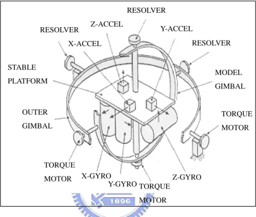
(23) Chapter 3. Inertial Navigation System. Inertial Navigation System (INS) has been developed for a wide range of vehicles. In general, an INS is mainly built up by a set of inertial measurement units (IMU), which consists of accelerometers and gyros, and the IMU is mounted on a platform. Besides, a processor is required to transform the measured data of acceleration and angular rate into useful navigation information: position, velocity, and attitude. [3] However, INS inevitably has its disadvantage in the errors of position, velocity, and attitude, which are usually caused by alignment, measurement, calculation, and initial states and often accumulate and grow divergently with time in the integral process. Therefore, INS needs external sensor to compensate, and the most popular method is using GPS to correct the divergent error in INS. INS can provide continuously position interpolation during the period of receiving GPS signal. The other purpose of INS would be used in automatic car control and that is to provide the velocity of vehicle, then the velocity would be feedback to control the vehicle.. 3.1 System Overview There are two general types of INS, gimballed and strapdown, which will be described in this section.. 3.1.1 Gimballed System. Figure.3.1 shows the gimballed system, where the accelerometers and gyros are mounted on a stabilized platform system; hence, it is also called the stabilized platform system [18]. To be a stabilized reference coordinates, the gimbals should be well controlled and then isolated from the vehicle’ s motion. Furthermore, the 13.

(24) accelerometers can be horizontally aligned to get rid of the gravity effect by rotating the platform. Although the gimballed system has high accuracy, some disadvantages, such as complex hardware design, high cost, and large power consuming, make the design of this system difficult. RESOLVER RESOLVER. Z-ACCEL. Y-ACCEL RESOLVER. X-ACCEL STABLE. MODEL. PLATFORM. GIMBAL. OUTER. TORQUE. GIMBAL. MOTOR. TORQUE MOTOR. X-GYRO Z-GYRO Y-GYRO TORQUE MOTOR. Figure 3.1 The gimballed INS system. 3.1.2 Strapdown System Contrary to gimballed INS system, the accelerometers and gyros (IMU) are mounted on a platform fixed on the vehicle in strapdown INS (SDINS). The IMU can measure the acceleration and angular velocity of vehicle, which are used to calculate the variation of position, velocity, and attitude. In the computing process, numerical errors caused by integrating the accelerations and angular rates would be produced accumulatively and divergently. Besides, the calculation of DCM (Direct cosine matrix) and Euler angle is quite complicated such that a high-performance processor is often needed. Fortunately, the technology of processor has been increasingly improved and good enough to do this work. 14.

(25) It is known that the gimballed INS system, better than the SDINS in accuracy, is commonly adopted for long-term navigation. However, the SDINS is generally employed for short-term navigation due to its small size, low cost, power saving, and easy design. For car-navigation, Hence the SDINS is available for car-navigation, which requires short-term data, with external sensors, like GPS, which can compensate the disadvantages in long-term work.. 3.2 Coordinate Frames And Transformation In general, there are five coordinate frames commonly used in an inertial navigation system. This section will first briefly describe these five coordinate systems and then show two transformations, between body and navigation frames and between geodetic and Earth-centered earth-fixed frames.. 3.2.1 Coordinate Frames A. Body Frame The body frame, also called the vehicle coordinate frame, is symboled as b-frame. The measurements acquired by various inertial sensors can easily apply to the body frame. Usually, the body frame is rigidly attached to the vehicle’ s center of gravity and its three axes are conventionally defined along the forward, right, and down directions as shown in Figure. 3.2, especially when adopted for car navigation. xb. yb zb Figure 3.2 Body (Vehicle) coordinate frame 15.

(26) B. Navigation Frame [3] The navigation frame, denoted as n-frame, is also called local geodetic frame with origin fixed on the vehicle and three axes pointing to the true north, east, and down as shown in Figure. 3.3. Clearly, the navigation frame intrinsically moves with the vehicle and then it is not suitable for specifying the vehicle’ s position on the earth. In fact, this frame plays a main role to provide local north, east, down directions and velocities, which is useful for navigation systems with sensors generally aligned with the local horizontal and vertical planes. x = north(true) y = East. Equator z = down Prime Meridian. Figure 3.3 Navigation frame or tangent plane reference coordinate frame C. Earth-Centered Earth-Fixed (ECEF) Frame The earth-centered earth-fixed frame, which is symboled as e-frame, is constructed with origin at the earth’ s mass center and the three axes rotate with earth. Furthermore, WGS-84 (World Geodetic System, 1984) is one kind of ECEF frame. Besides, the x-axis and the y-axis respectively point to the prime meridian of 0o longitude and the meridian of 90o longitude through the tangent plane of the equator, and the z-axis points to North Pole as shown in Figure. 3.4.. 16.

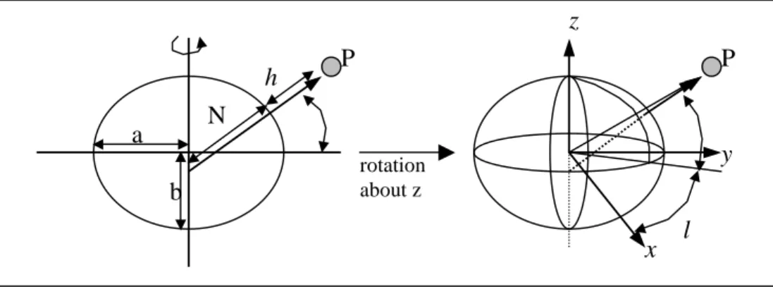
(27) z Prime meridian. y. Equator plane. x. Figure 3.4 ECEF rectangular coordinate system D. Geodetic Frame The geodetic frame, which is symboled as g-frame, describes the position of a moving body by the longitude, latitude, and altitude, denoted as l, L, and h, where the 0o longitude is defined at Greenwich meridian and the 0o latitude is defined at the equator. The meridian longitudes start from 0o longitude at Greenwich meridian to the west and the east each up to 180o and the parallel latitudes start from 0o latitude at the equator to the north and the south each up to 90o. The altitude is defined as a distance from the local sea level to the point where the vehicle locates as shown in Figure 3.5. z h. P. P. N. a b. y. rotation about z. x. l. Figure 3.5 Geodetic reference coordinate system E. Inertial frame This frame is the most fundamental coordinate system that is symboled as i-frame and defined in which Newton’ s laws of motion apply. The frame is static or in uniform linear motion system without accelerating. The definitions of axes are 17.

(28) generally built base on the star in universe. The x and z axes point toward the vernal equinox and along the earth’ s spin axis. The y-axis is defined to complete the right-handed coordinate system. In this analysis, the frame is attached to the center of earth, and is not rotating.. 3.2.2 Transformation Between ECEF and Geodetic Frames This section will discuss the transformation between ECEF and geodetic (Longitude, Latitude, and Altitude)[17]. Besides, the WGS-84 ellipsoid parameters are used throughout this discussion. The position in the ECEF frame is calculated as follows.. x  N h   cos L  cos l. (3.2.1). y  N h   cos L  sin l. (3.2.2).   . z  N 1 e 2 h  sin L. (3.2.3). N  L . (3.2.4). where a 1 e 2 sin 2  L. Semimajor axis length: a 6378137.0m Semiminor axis length: b 6356752.3142m Eccentricity: e 0.0818 In GPS application, the range measurements of GPS receiver are determined in ECEF frame. However, the information of geodetic frame is more useful in navigation. Therefore, the transformation between ECEF and geodetic frame is desired to solve. Longitude (l) can be solved as. 18.

(29) l arctan 2 y, x . (3.2.5). The solutions of h and L can be computed by iterations as follows: A. Initialization: Let h 0 N a. . p  x 2 y 2. . B. Perform the following iteration until convergence: z sin L  N 1 e 2 h.   z e Nsin L arctan L /p  2. N. a 1 e 2 sin 2  L. p h N cos L. 3.2.3 Transformation Between Body and Navigation Frames In vehicle navigation application, the relation between body frame (x, y, z) and navigation frame (N, E, D) is shown in Figure 3.6. This relation exists angular motion between body and navigation frame. Therefore, the transformation between them will be discussed in this section. N. E. x. Tangent plane. y z D. Figure 3.6 Relation between body and navigation frame 19.

(30) Consider the three rotations involving the Euler angles  φ, θ , ψ =(roll, pitch, yaw). A. Rotates the navigation frame by ψ radians about the D axis as shown in Figure 3.7 (a). x N   cosψ sinψ 0   y      sinψ cosψ 0    E     0 1 D z     0   . (3.2.6). B. The second rotation rotates the coordinate that resulted from previous yaw rotation by θ radians about the y axis as shown in Fig 3.7 (b).. N. . x.  x x . E.  D,z.  x ,x. y.   z.  y , y. z. (a). (b).  y .  y z   z (c). Figure 3.7 Rotation by the Euler angles  x cosθ 0 sinθ x      y         1 0    0 y       sinθ 0 cosθ z      z  . (3.2.7). C. The third rotation rotates the coordinate that resulted from previous pitch rotation axis as shown in Fig 3.7 (c). by φ radians about the x .  x  1 0 0  x    y       0 cosφ sinφ   y      0 sinφ cosφ z      z  . (3.2.8). 20.

(31) The vector represented in tangent-plane coordinate can be transformed into body-frame by the transformation described as x N   y C b E   t     D z    . (3.2.9). where 1 0 0  cos  0 sin    cos sin 0      C  0 cos  sin  1 0  sin cos 0 0         0  sin  cos  sin  0 cos  0 0 1       b t.   coscos   sincos    cossin sin   sinsin    cossin cos  .  sincos  sin    coscos  cos sin   sinsin sin   cossin  cos cos   sinsin cos  . (3.2.10). Furthermore, the transformation C bt is determined as  C tb . T. 3.3 Dynamic Equations in Navigation Generally, navigation problem is based on integrating sensed accelerations and angular rates to solve position, velocity, and attitude. In n-frame, there are a lot of differential nonlinear equations, based on the dynamics of motion according to Newton’ s Law, which can be formulated and constitute dynamic equations. In this section, the dynamic equations will be derived. In order to realize the dynamic equations, two fundamental concepts and properties should be discussed and expounded, and then dynamic equations can be derived easily.. 3.3.1 Coordinate Transformation Matrix Properties 21.

(32) Consider the position of a point represented by a-frame and b-frame. The transformation of the a-frame to b-frame can written as r b C ab r a. where. (3.3.1). r a and r b are respectively the position vectors in a-frame and b-frame and. C ab is the transformation matrix, called the direct cosine matrix (DCM).. There are two properties used in dynamic equations and described as: A. The time derivative of the transformation matrix is given by:. C ab  ΔC ab C ab  t Δt t b C  lim  lim a t 0 Δ t t 0 Δt. (3.3.2). . (3.3.3). C ab  t Δt C ab  t I Δa. . where I a. . is the small angle transformation relating the a frame at time t to. the rotated a frame at time tΔt. Then substituting (3.3.3) into (3.3.2) Δa b b C  C  t  lim a a t 0 Δ t. (3.3.4). define Δa lim baa t 0 Δ t where baa is the angular velocity of the a frame w.r.t. the b frame, with coordinates in the a frame. Consequently b b a C a C a ba. (3.3.5). a where baa denotes a skew-symmetric matrix with elements from ba .. 22.

(33) 0    ωz  ωy  a ba.   a ba. ωz 0 ωx. ωy   ωx  0  . (3.3.6). B. Since the columns of C ab are mutually orthogonal, as are the rows. Therefore the matrix C ab is an orthogonal matrix, i.e..   C . C ba  C ab. 1. b T a. (3.3.7). For any 3-by-3 matrix, A a , under an orthogonal frame transformation can be derived as follows. Let r a A a r a . From the transformation between coordinates described in (3.3.1) and the property derived in (3.3.7), we have r b C ab A a C ba r b. (3.3.8). From (3.3.8), it follows that A b C ab A a C ba. (3.3.9). These two properties would be useful in deriving dynamic equation. Furthermore, the next section would start the derivation of velocity dynamic equation.. 3.3.2 Velocity Dynamic Equation After the necessary properties (3.3.5) and (3.3.9) are given, the derivation of the velocity dynamic equation could be started from measuring the specific force in motions based on the Newton’ s law. First, let’ s consider the force exerted on the system in the inertial coordinate. 23.

(34) frame, say i frame [9, 10], which is obtained as i  f i r G i. (3.3.10). where r i and G i represent the positional vector and gravitational acceleration at the system, respectively. Now define the position vector and velocity vector in the navigation. coordinate. v n  vN. vE. frame,. say. n. frame,. as. r n  rN. rE. rD  and. v D . Further applying the transformation between two different. coordinates shown as (3.3.1), we have r e C ie r i. (3.3.11). e v n C en r. (3.3.12). where the super indices e and n denote the Earth coordinate and navigation coordinate. Substituting (3.3.11) into (3.3.12) leads to. . n i e i v n C e C ie r C i r. n. . . i C e C ie r C ie eii r i. . . . . i C in r eii r i. i C in r iei r i. . (3.3.13). The time derivative of (3.3.13) is given by n i n i n i i i i r i  C v C in  r C C in iei r C in  i r  i ie r  ie.  . . . i i i r i C in  r iei ini r ini iei r i C in  ie. (3.3.14). i 0 , it is attained that Since iei C ni ien C in , ini C ni inn C in and assume  ie. . . . n i i  v C in r C ni ien inn C in r C ni inn C in C ni ien C in r i. . . i i C in  r ien inn C in r inn ien C in r i. 24. .

(35) From (3.3.13) and (3.3.1), we have. . . . .  . . .  . . . . n i v C in  r ien inn v n C in iei r i inn ien r n. . i C in  r ien inn v n ien inn C in C ni ien C in r i inn ien r n. i C in  r ien inn v n ien inn ien r n inn ien r n. i C in  r ien inn v n ien ien r n. (3.3.15). Pre-multiplying (3.3.10) by C in yields i f n C in  r G n. (3.3.16). Substituting (3.3.16) into (3.3.15) shows that. . . . n v ien inn v n f n G n ien ien r n. where. . (3.3.17). ien ien r n represents the centripetal acceleration.. -r. Figure 3.8 Gravitational acceleration vector in the navigation frame Define the gravity vector in the n frame as g n G n ien ien r n. (3.3.18). then (3.3.17) would be rewritten into. . . n v ien inn v n f n g n. (3.3.19). where ien v n ien v n , also note that ien , inn represent the Earth rate vector and the angular rate respectively in the n frame relative to i frame. Traditionally,. 25.

(36) ωe sinL 0 ωe cosL   0        0  ωe sinL 0 ωe cosL         ω sinL 0 ω cosL 0 e  e    n ie. n ie.  . ωe lcosL   0    inn inn  L  ωe lsinL     ωe lsinL     L.  .  . ω lsinL.  L  0 ωe lcosL   ωe lcosL 0  e.  .  . Hence, (3.3.19) could be expressed as the following the state-space form:. . . . . n    v 0 2 ωe lsinL N n   v 2 ωe lsinL 0 E   n    L v 2 ωe lcosL D  . . .   L v Nn  f Nn  0   n   n    2 ωe lcosL  v E f E 0     n  0 v Dn  gn    f D   . . . (3.3.20) Consequently, (3.3.19~20) are the velocity dynamic equations useful for inertial navigation and autonomous control of vehicle. In addition, the relation between n and geodetic frames is shown as  v Nn   ρM h n   v E  0   v Dn   0   .   0 L     ρp h  cosL 0  l    0 1 h    0. (3.3.21). or  1  ρM h    L    l  0    h   0  . 0 1  ρP h  cosL 0.  0  v Nn   n  0 vE     v Dn    1  . where.  e2 2  ρM a  1 e  sin 2 L 1 R  2 . . .  e2  ρP a  1  sin 2 L R  2  26. (3.3.22).

(37) With the dynamic equation in (3.3.20) and the relations in (3.3.21-22), the INS dynamic equations are more complete. In next section, the INS error model would be introduced to realize how the errors affect the INS system performance.. 3.4 INS Error Model The inertial navigation system is a rather complex instrument whose components would affect the system errors due to initial random errors and modeling errors. Therefore, in order to understand the influence of the system errors in navigation solution, it is important to develop the dynamic and stochastic models for these system errors.. 3.4.1 Error Model How the sensor errors affect the position and velocity is described by the dynamic error model which be derived by applying a differential operator to the dynamic navigation equations. That is, the variables of the navigation equations are perturbed differentially. There are two approaches generally employed to derive dynamic error model: perturbation approach and psi-angle approach [4]. First, from (3.3.22) the use of perturbation approach would give the dynamic error model as  1    ρM h δL    δl  0  δ h   0  . 0 1 ρP h cosL 0.  L   0   ρM h   δ v    0   N    l    0 δ vE   δ h l tan L δ L    (3.4.1)   ρP h      δ vD    0  0  1        . In this thesis, the psi-angle approach is adopted and the dynamic error model is. 27.

(38) represented as [4] n δr ρδr n δv n. . (3.4.2). . n δv ien inn δv n δf n g n. (3.4.3). inn δ  δ. (3.4.4). where. v : velocity error vector. r : position error vector..  : attitude error vector.  : accelerometer error vector.. g : error in the computed gravity vector..  : gyro drift vector. ρ : rotation rate vector of the navigation frame w.r.t. the Earth.. The state space form of (3.3.2~4) is given as. XI AI X I B I. (3.4.5). where. X I  δrN A11 AI  A21  033 . δrE I 33 A22 033. δrD. δ vN. δ vE δ vD. 033  A23   A33   99. 0 l sinL L    A11  l sinL 0 l cosL  L l cosL 0   . 28. δ ψN. δ ψE. δ ψD  T.

(39) g/R 0 0    A21  0 g/R 0     0 0 2 g/R  . . . . .  0 2 ωien lsinL  A22 2 ωien lsinL 0 n   L 2 ωie lcosL . . 0 A23  f D  f E . . f D 0 fN. . B I  0 0 0 N. . . fE  f N   0  . . . . .  0 ωien lsinL  A33 ωien lsinL 0 n   L ωie lcosL . .  L  n 2 ωie lcosL   0 . E. D. ε N.  L  n ωie lcosL   0 . . . ε ε E D T. Actually, there exist stochastic characteristics in sensor. Therefore, in the following section, the stochastic model of sensors will be derived and expounded.. 3.4.2 Error Sources The major error sources of INS are gyro and accelerometer, and furthermore their bias and scale factor error are not always white noise. In this section, the principle work is to discuss these sources and model these errors, so that the INS error model would be completely expounded. The discussion can be separated into two parts: gyro and accelerometer [19~21]. In general, gyro has four types of error, such as random bias B g , scale factor SFg , random drift ε g , and random noise w g . The instrument specification can be. described as:. 29.

(40) B g ε ψ g w g SFg ω. where. (3.4.6).  represents the output of the gyro ψ. ω represents the angular rate of the vehicle. These four types of error can be modeled as:. B g 0 SF g 0 E ε 0 g 2 E ε t  ε τσε δ t τ  g g  g. wg wg /τ g w gn. where. g is the correlation time of random noise wg . E w g n 0. E w gn  t  w gn  τσw2 gn δ t τ  2 Q gn  2 σgn /τ represents the power spectrum of wgn g. Therefore, the gyro errors can be modeled as:. Xg Ag X g w1. where. X g  w gN. wgE. (3.4.7). wgD. B gN. B gE. 30. BgD. SFgN. SFgE. SFgD.  T.

(41) 1 / gN   0 Ag   0  . . w1  w gnN. 0 1 / gE 0 063. w gnE. wgnD. 0 0 1 / gD.  036     066 . 0 0 0 0 0 0.  T. As the same discussion above, the instrument specification of accelerometer can be expressed as vΔBa SFa f where. (3.4.8). v represents the output of accelerometer. Δ represents the random drift. Ba represents the random bias SFa represents the scale factor f. represents the acceleration of vehicle. The accelerometer errors can be modeled as SF a 0. E Δ 0 2 E Δ t  Δ τσΔ δ t τ . B a B a /τ a wa. where. a represents the correlation time of random bias. 31.

(42) E wa 0.  E wa  t  wa  τσw2 a δ t τ Qa  2 σa2 /τ represents the power spectrum of wa a Thus, the accelerometer errors can be modeled as:. Xa AaX a w 2 where. X a  BaN. BaE. 1 / aN   0 Aa   0  . w 2  waN. waE. (3.4.9). BaD. 0 1 / aE 0 033. waD. SFaN. SFaE. SFaD  T.  033     033 . 0 0 1 / aD. 0 0 0 T. With the discussion of errors in IMU (3.4.7~9), the dynamic error model mentioned in (3.4.5) would be extended to 24 state variables and shown as. XAX B where. (3.4.10). X  r v   wg   AI 99     A 099     069  . 033 033 I 33. Bg. SFg. 033 033 033 033 I 33 33. 033 I 33 033. Ba. SFa. 033   f 33  033    096      Aa 66   . Ag 99. 069. 2424. 32.  T.

(43) . B 0  g. w gn. 0 0.  T. wa. 0 124. Consequently, this INS error model composed of dynamic and stochastic models describes how the dynamics equation and sensor errors propagate through the system into navigation errors.. 3.4.3 The Reduced Error Model In this subsection, the reduced error model for this system will be described. From the error model in (3.4.10), the state variables X of the model can be reduced as to the following form.. X A X  B . (3.4.11). where. X   rN  0 l sin L  0 l sin L  g / R 0  g / R  0  0 0 A  0 0  0  0  0 0  0 0   0 0 . rE. V N. V E. 1 0.   wg. Ba. 0. 0. 0. 1. Bg. SFg. . 0. 0. 0. SFa. T. 0. 0. 0. 0. 0. 0 2 lsin L. 2 lsin L. fE. 0. cos. 0. fN. 0. f N. 0. sin. 0. fE. 0. 0. 0. 1. 0. 1. 0. 0. 0. 0. 1 / g. 0. 0. 0. 0. 0. 0. 0. 1 / a 0. 0. 0. 0. 0. 0. 0. 0. 0. 0. 0. 0. 0. 0. 0. 0. 0. 0. 0. 0. 0. 0. 0. . . n ie. . n ie. . 0  0 0  0   0  0 0  0 0  10 10. where B  = the input noise vector.. . B 0 0 N. E. g w gn. wa. 0 0 0.  T. Which has zero mean and with covariance as. . 2 Q diag 0 0  N. 2E. 2g w2 gn. w2 y. 0 0 0. . This reduced form is used in Kalman filter, and next; the general form of Kalman filter will be discussed. 33.

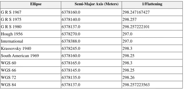
(44) Chapter 4. Geographic Information System. 4.1 Introduction The Federal Interagency Coordinating Committee defined the term Geographic Information System in the following manner: “A system including computer hardware, software, and procedure, which is designed to support the capture, management, manipulation, analysis, modeling, and display of spatially referenced data for solving complex planning and management problems”in 1988. Such a system is an electronic spreadsheet coupled with powerful graphic-manipulation and display capabilities. In general, a geographic information system (GIS) combines graphic system and data processing system to manage the graphic data, characters, numeral data, and attribute data. Attribute data is associated with the graphic data and provide more descriptive information about them. Therefore, GIS can give not only the information of the data element itself, but the nearby information. [26]. 4.2 Reference Ellipsoids and Projection This section would describe the reference ellipsoids, which would be used in projection and coordinate transformation. Ellipsoidal models define and ellipsoid with an equatorial radius (semi-major axis) and a polar radius (semi-minor axis) that is shown as figure 4.1. There are three kinds of reference ellipsoid parameters shown as table 4.1. Reference ellipsoids used with different nations and agencies are shown as table 4.2. To transform three-dimensional space onto two-dimensional map is called “ Projection” . Projection formulas convert a geographical location on sphere or spheroid to a representative location on flat surface. There are three commonly. 34.

(45) North Pole Polar Radius (Semi-Minor Axis) = b. Equatorial Radius (Semi-Major Axis) = a. Equator. Figure 4.1 Semi-major axis and semi-minor axis Table 4.1 Ellipsoidal Parameters Ellipsoid Parameters. Functions a b f  a 2 2 a b e 2  2 2 f f 2 a a 2 b 2 2 e  2 b. f (Flattening) e 2 (First Eccentricity Squared) 2 e (Second Eccentricity Squared). Table 4.2 Selected reference ellipsoids Ellipse. Semi-Major Axis (Meters). 1/Flattening. G R S 1967. 6378160.0. 298.247167427. G R S 1975. 6378140.0. 298.257. G R S 1980. 6378137.0. 298.257222101. Hough 1956. 6378270.0. 297.0. International. 6378388.0. 297.0. Krassovsky 1940. 6378245.0. 298.3. South American 1969. 6378160.0. 298.25. WGS 60. 6378165.0. 298.3. WGS 66. 6378145.0. 298.25. WGS 72. 6378135.0. 298.26. WGS 84. 6378137.0. 298.257223563. 35.

(46) projections, azimuthal projection, cylindrical projection, and conical projection shown as figure 4.2. Azimuthal projection can be classified into three types based on the difference of the projected origin shown as figure 3.6.. Cylindrical. Azimuthal. Conical. Graticules :. Figure 4.2 Projections and the appearance of the Graticules. C. A: Gnomonic (from center of the Earth) B: Stereographic (from a diameter’ s distance). A. B. C: Orthographic (from infinity) C. C. Figure 4.3 Azimuthal projection. 36.

(47) 4.3 Taiwan Coordinates The conventional geodetic datum used in Taiwan was based on the geodetic observations carried out in 1978, and the reference ellipsoid was the Geodetic Reference System 1967 (GRS67). The origin point of this datum locates at the Hu-Tzu-Shan astronomic station. The coordinates, which includes the latitude and longitude based on the GRS67, grid coordinate based on 2。-Zone Transverse Mercator (TM) projection, and the height is above the mean sea level. The set of coordinates adopted in Taiwan was called the Hu-Tzu-Shan coordinate system, and also named the TWD67 (Taiwan Geodetic Datum based on the GRS67). [27] The recommendations made by the IERS (International Earth Rotation Service) also encourage national agencies to establish their precise national datum based on the ITRF (International Terrestrial Reference Frame). This datum would be linked into regional or continental solutions and employed for many international applications. Thus, a geodetic ellipsoid, GRS80, was adopted with the new national coordinate system called the TWD97 that also employs the Transverse Mercator. Table 4.3 shows the parameters of TWD67TM2 and TWD97TM2 coordinates in Taiwan. The grid coordinate is calculated with a 2-degree zone and 121。E and 119。E. Furthermore, the western offset of the transverse axis is 250,000 m and the scale ratio is 0.9999, where the scale ratio is defined as: Scale ratio=actual map scale/nominal scale. Table 4.3 Taiwan coordinates Coordinates. Reference Semi-Major 1/Flattening Ellipsoids Axis. Central Meridians. Western Offset. Scale Ratio. TWD67TM2. GRS67. 6378160.0. 298.247167427. 121°E,119°E. 250,000 m. 0.9999. TWD97TM2. GRS80. 6378137.0. 298.257222101. 121°E,119°E. 250,000 m. 0.9999. 37.

(48) 4.4 Map Matching Algorithm The purpose of the map-matching algorithm is to locate the position of the vehicle on the map. Since the GPS satellite signal has errors and noise due to the tropospheric and ionospheric propagation delays, and GIS database is more accurate. Therefore, a map-matching method using a digital map is a useful approach to correct these errors. Furthermore, the fact that “A vehicle moves always on a road network. ” makes the utilization of the map information more effective. With the assumption that land-vehicle almost run on roads, most of vehicle navigation systems translate the GPS position onto a road, and the position errors can be eliminated if the road where the car locates can be found. In other words, the map-matching problem can be defined as the identification problem of the road where the car locates. Furthermore, the map-matching function would integrate measured position and the digital map data to locate the vehicle on proper position relative to digital map. There are several criterion used in the map-matching function and described in the following sections.. 4.4.1 Map Matching Issues There are three issues that would be discussed in the map-matching algorithm and presented as the following description. Projected error is defined as the distance between the measured position obtained from the GPS/INS and its projected position on the road shown as figure 4.4. Therefore, the first issue of the map-matching algorithm is that the projected error must be small, so that the correct located road would be found. The dot-product implies the similarity between the shape of the road and the trajectory of the vehicle shown as figure 4.5. Thus, the second issue of map-matching algorithm is that the dot-product value should be big, so that the vehicle would be matched to the correct road due to the fact that the trajectory is similar to the shape of road. The definition of the moving distance is the distance 38.

(49) between the present vehicle position and the previous vehicle position shown as figure 4.6. Accordingly, the third issue is that the difference between the moving distance and the projected moving distance should be small. Consequently, these three issues would be useful to decide which road the vehicle runs. Next section would discuss the map-matching structure and give the flowchart. [11] Received position Road Projected error. Projected position. Figure 4.4 Projected errors.  A.  A  B.  C.     A B A C    where A  B C. Figure 4.5 Dot-product Received position. Moving distance. Projected moving distance Projected position. Figure 4.6 Moving distance 39.

(50) 4.4.2 Map Matching Structure In the map-matching structure, three modes are used and they are initial mode, searching mode, and tracking mode. In the initial mode, only the projected error measurement is used, and the first issue would decide the closest road and the closest point. As the vehicle starts to run, the navigation system would detect how many nodes, which are the junctions of two or more roads, are near the vehicle. If there were nodes nearby, the mode would be changed to the searching mode. As the matched road and matched point are decided, the mode would back to the nodes nearby decision. If there is no node nearby, the mode would be changed to the tracking mode, and that means the vehicle position approaches only one road. Then, the projection method would be employed to decide the projected point of the initial road or the previous matched road. Furthermore, the mode would also back to the nodes nearby decision after the projected point is calculated. The complete map-matching flowchart is shown in figure 4.7 and the detail procedure of the map-matching structure is presented in the next four sections. Start. Initial Mode. Nodes nearby?. Tracking Mode No. Yes. Searching Mode. Figure 4.7 Map matching flowchart 40.

(51) 4.4.3 Initial Mode The projected error and first issue are used to determine the closest road and the closest point in the initial mode. The initial mode includes three steps: 1. Search the roads in the range of 150 m. 2. Find the closest road. 3. Find the closest point on the closest road. Figures 4.8 shows that the navigation system would search the roads around the measured position and find the closest road and point.. Searching range. Figure 4.8 Initial mode. 4.4.4 Nodes Nearby Detection and Searching Mode The node nearby detection is always applied when a new measured position is obtained. The node nearby detection is used to judge that the next mode is the searching mode if there are nodes nearby or the tracking mode if there is no node nearby. In addition, the searching range of this detection is 20 m. In searching mode, these three issues have different processing priorities respectively. The projected error has the highest priority, and the moving distance has the lowest priority. As the GPS/INS position is obtained in the searching mode, the system would search the candidate roads with searching range of 20 m. If there is only. 41.

(52) one candidate road, the projection method is adopted only. If there are more than one candidate roads, the dot-product operation is employed. From the second issue of the map-matching algorithm, the road that has the biggest dot-product value is the matched road. However, if the difference between the two biggest dot-product values were smaller than 0.1, the moving distance judgment would be applied to decide the matched road. The complete flowchart of the searching mode is shown in figure 4.9. Start. Search for cadidate roads. Only one road ?. Yes. Projection Method. No End Condition1. Dot-product Operation. Difference <0.1. Yes. Moving Distance Judgement. No End Condition 2. End Condition 3. Figure 4.9 Searching mode flowchart There are three conditions in the searching mode shown as figure 4.9. In condition2, there are 7 steps to match the right road shown as figure 4.10: 1. Search the candidate roads in the range of 20 m. 2. List the candidate roads (road1 and road2). 3. Find out the projected points according to two roads ( c1  k , c2  k ). 4. Transfer to the unit vector form. 42.

(53) p k p k 1  p k  p k p k 1. (4.4.1). c  k s  k 1  c1  k  1 c1  k s  k 1. (4.4.2). c  k s  k 1  c 2  k  2 c2  k s  k 1. (4.4.3). 5. Perform the dot-product operation and find out the biggest one..     p k c 1  k p k c 2  k. (4.4.4). 6. The c1(k) and road1 are chosen to be the matched point and matched road. From figure 4.10, there are two candidate points c1(k) and c2(k) and they are almost possible to be the matched point. As the dot-product is applied, it is clear that the c1(k) is the right matched point.. road2. p k 1. p k 2 . s k 2 . s k 1. p  k. c2  k. road1. c1  k. Received GPS position Map-matched point Candidate point Searching range for nodes Searching range for roads. Figure 4.10 Condition 2. In condition 3, the moving distance judgment is adopted to decide the matched point.   and road finally. From the figure 4.11, the difference between p k c 2  k and   p k c1  k is smaller than 0.1, but when the moving distance judgment is used as: c2  k s  k 1 p  k p  k 1 c1  k s  k 1 p  k p  k 1(4.4.5). Consequently, the c1(k) and road1 are decided as the matched point and road. The overall searching mode has been presented; the next section would introduce the tracking mode employed as there is no node near the vehicle. 43.

(54) 4.4.5 Tracking Mode As map-matching function enters the tracking mode, this expresses that there is only one road. Therefore, the matched road would be the initial road from the initial mode or the previous road. Furthermore, the projection method is applied to decide the matched point on the tracking road shown as figure 4.11. The entire map-matching algorithm has been expressed in section 4.4, and the performance of this algorithm would be tested in the experiment described in section 5.5.. Searching range for nodes. Figure 4.11 Tracking mode. 44.

(55) Chapter 5. Integration of GPS/INS/GIS. 5.1 Motivation With the description of previous sections, it is clear that GPS, INS and GIS have complementary characteristics. These characteristics, which motivate the integration of navigation system, can be summarized as [22]: I.. Accuracy: Due to the integral of acceleration and angular rate involved, as estimating position, the INS would produce unbounded grown error over time. This gives the requirement in correcting the errors periodically by external sensor. GPS, with bounded measurement errors, can be used to accomplish this work. Furthermore, GIS has most accurate precision database, which can associate GPS to improve the accuracy.. II.. Data Output Rate: The data output rate of GPS is generally 1Hz that can’ t satisfy the request of autonomous control of vehicle. The INS output rate can be higher, but the only limit being the ability of data processor. Therefore, the integration of GPS and INS is sufficient for the data output rate requirement.. III. Data Availability: GPS is a radio-navigation system, and consequently its measurement is subject to the signal outage, interference, and jamming. On the contrary, INS is a self-contained and much immune to surrounding environment. Hence, INS can provide available and continuous navigation information when GPS loss signal in short-term time. On the other hand, GIS may disable while roadways have been developed or pulled down, and furthermore the GIS database has not update recently. However, GPS/INS would show the trajectory that vehicle passed through but the roadway. 45.

(56) doesn’ t exist in GIS database. As the compensated characteristics of each element have been presented clearly, the integration of GPS/INS/GIS would be possible to achieve a more efficient, robust, and accurate position estimate.. 5.2 Integration Mode In this application, there are three components of navigation, GPS, INS, and GIS, whose characteristics are complementary. In order to achieve the optimal performance, such as availability, reliability, and accuracy, the proposed procedure is to integrate them. The overall integration would be divided into two parts, one is GPS/INS and the other one is GPS/INS/GIS. As absolute position has been determined in GPS/INS, then the relative position in map would be matched from GPS/INS/GIS. In GPS/INS integration, one Kalman Filter, which would be introduced in section 5.3, is used to combine two different data output rate systems, GPS and INS. Figure 5.1 shows the integration procedure that as the INS estimates the P+ P and GPS measures the P/+, and then the difference would be input into the Kalman Filter to get the optimal error dP/. After that, the output of INS may subtract the optimal error and get the optimal navigation.. INS. Optimal navigation information. +. P+ P. Position, velocity, and heading. dP/. -. GPS Position, velocity, and heading. + Kalman. P + /. Filter. Figure 5.1 GPS/INS integration scheme While the position, velocity, and heading direction shown in figure 5.1 have. 46.

(57) been estimated, the next work would make effort in providing the correct geographic information for driver. Compare GPS, INS, and GIS, the GIS database is the most accurate due to the precise data establishment, thus the GIS is considered to fix the GPS/INS position. While using the map-matching algorithm, a GIS position correction method is proposed to fix the position determined from GPS/INS. If the absolute positions of GPS/INS just match to the relative positions on the road without correcting from GIS, the GPS/INS estimation error would cause the wrong matching shown as figure 5.2.. GPS/INS position GIS matching position. Practical trajectory. Figure 5.2 GPS/INS without GIS fix Thus, the proposed method would match the present GPS/INS position to the correct position on the located road, and then the next heading direction estimation would be determined base on the heading direction measured from GIS shown in figure 5.3 (b). Since the vehicle runs in the road, the heading direction is similar to the direction of the road. The direction of road would be used to fix the heading direction. However, as the vehicle has a turn, the GIS heading direction fixing would fail and be shown as the left of figure 5.4. Because the direction of road doesn’ t vary as the vehicle run in the same road. Therefore, an improved method is to detect if there is a node near the vehicle and the variation of direction measured from INS; if yes, then the GIS heading direction fixing wouldn’ t work until there isn’ t node near the vehicle 47.

(58) and the vehicle and the variation of direction from INS is small. This method is shown in the figure 5.4 (b).. (b). (a) Heading direction without GIS correction GPS/INS position. GIS fix the position, velocity, and heading. GIS matching position. Practical trajectory. Heading direction. Figure 5.3 GIS fix GPS/INS. Turn Detect Range Direction error. (a). (b) Turn Detect Range. GIS heading direction fixing GPS/INS position. GIS matching position. Heading direction. Practical trajectory. Figure 5.4 Turn Detect Range As the heading direction has been fixed with GIS, the trajectory would be shown as figure 5.5. This trajectory of GPS/INS/GIS shows the more correct road information than the one of GPS/INS. Furthermore, as the GIS aid the GPS/INS, there 48.

(59) would be two conditions in real environment shown as in figure 5.3. As GIS is available, i.e. the road that the vehicle passes through exists, there would not be any error message.. Turn Detect Range. GPS/INS position. GIS matching position. Heading direction. Practical trajectory. Figure 5.5 GIS fix GPS/INS. Start. GPS initial. GPS. INS. GPS/INS with Kalman Filter. correct. Car controller. position, velocity attitude unavailable Draw the trajectory. GIS Map-matching. 1 Hz. 1 Hz. Display. Figure 5.6 GPS/INS/GIS integration mode 49.

(60) However, if the vehicle passes through the road that have not been updated in GIS database, the navigation information would depend on the GPS/INS and show the trajectory without the located road information. Figure 5.6 interprets the overall integration mode, and further the output of GPS/INS, such as position, velocity, heading direction, could be also used in car control.. 5.3 Filter Design In navigation system, it is required for estimation to obtain position, velocity and attitude, modeled in (3.3.19) and (3.3.20). Further using psi-angle approach results in error models as shown in (3.4.11). In order to achieve the best estimates, most researchers relied on Kalman Filters, which is a recursive algorithm and requires external measurements to compute optimal corrections of system state variables. This application also includes a GPS as the external measurement, possessing tens of meters in position uncertainty. Thus, the main work of GPS/INS would be devoted to the design of the Kalman Filter, which provides the optimal navigation information.. 5.3.1 Discrete Linear Dynamics Model and Observation Model Consider the INS reduced error model in (3.4.11) that is a nonlinear system, and is needed to reformulate discrete-time form for Discrete Kalman Filter. In error model, it is assumed that for small time intervals, the dynamic matrix Ais constant. The state-transition matrix  is given as: [3].  e At .. (5.3.1). Identifying t 0 t k 1 and t t k , and then the discrete random process uk with Gaussian, zero-mean white noise is given by uk  t,t   B  t dt  . tk. (5.3.2). t k 1. 50.

(61) Thus, the discrete error model can be given by δX k t k ,t k 1  δX k  1 u k . The X k and uk. (5.3.3). posteriori density are Gaussian and their covariance are. respectively given as. . . T Pk E X k X k ,. (5.3.4).  . Q k E uk ukT .. (5.3.5). In (5.3.3), it describes the discrete linear dynamics model in a small time interval and would estimate the error state by sensed values from integrating the IMU sensor output. Except for estimating error state by error model, the external measurement, GPS, can also obtain more accurate error at 1Hz. In this application,  Yk might be the difference between measurement in GPS and estimation in INS, and they are also 5 observations linearly related to the state through the matrix H k shown as following: rNGPS rNINS   GPS INS  rE rE  δYk  VNGPS VNINS H k δX kv k .  GPS  VE VEINS    ψGPS ψINS    1   0  H k  0  0   0 . (5.3.6). 0 0 0 0 0  0 1 0 0 0 0  0  0 1 0 0 0  0 .  0 0 1 0 0  0 0 0 0 1 0  0  5 10. v k ~ Ν 0 , Rk  where V NGPS is the north velocity measured from GPS and V NINS is the north velocity estimated from INS. In order to estimate the optimal error estimation, Kalman Filter combines the observation model with dynamic error model to integrate them. 51.

(62) Consequently, the estimation of state error using the observations is called the update, and the step based on the system dynamics error model is called the prediction.. 5.3.2 Optimal State Vector Estimation Before starting to compute the optimal estimation, some important symbols would be given expositions. An estimate of the state error is denoted with “ ^” . There would be a distinction between if an observation were included. Let δXˆkbe the  estimate at time t k , just after including the observation δYk ; and let δXˆk be the. estimate just prior to the inclusion of the observation. With these preliminaries, optimal estimation can be started in two steps: prediction and filtering. In many applications, the true values of system states are not known. However, it is assumed that the mean of the initial optimal estimate is known and given as. δXˆ0E  δX 0 . (5.3.7). With the same assumption, the initial covariance of the system is. . . P0 E δX 0δX 0 T. (5.3.8). For convenience in further discussion, the errors in estimation can be shown as. e 0 δXˆ0δX 0. (5.3.9). where e0~ N  0, P0  . The states and errors ( δXˆk , e 0 ) are assumed to be Gaussian. According to the state transition matrix,  , the states can be propagated to the expected value based on all prior information.  δXˆk E  δX k . (5.3.10).  t k ,t k 1  E δX k E  uk   1.  t k ,t k 1  δXˆk  1. 52.

(63)  where δXˆk is the estimate error state in prediction prior to the use of new. information and this is the known prediction. Then, let the estimation error be  e k δXˆk δX k. (5.3.11). Similarly, the estimation error and its covariance are propagated from (5.3.10), thus the error is e k  t k ,t k 1  e k 1 uk. (5.3.12). Covariance matrix of error would start to determine from P0 .. . Pk E e ke kT  t k ,t k 1.  E  e. (5.3.13).  T k 1 k 1. e.    t ,t T. k. k 1. E  uk ukT .  t k ,t k 1  Pk 1T  t k ,t k 1  Q k. Note that Pk 1 has non-negative diagonal elements, as dose Q k . Thus the variance of system states would increase due to the driving noise variance. Furthermore, the probability density of estimation error is Gaussian..  . e k ~ N 0 , Pk. (5.3.14). A simple prediction is completed with available information, model, and gives the best estimation without external information. Once new information is measured, it is important to employ this information to find the best estimate and then remove the error of prediction. This process is known as filtering. The best posterior estimate of error states based on the observation is combined with both the prior best estimate established in prediction and a weighting difference between the observation and the prior best estimate. In this thesis, the following algorithms will be adopted:. . .   δXˆkδXˆk K k δYk H k δXˆk. (5.3.15). Pk  I K k H k  Pk I K k H k  K k Rk K kT. (5.3.16). T. where. . K k PkH kT H k PkH kT Rk.  1. 53. (5.3.17).

(64) and then combined with (5.3.10)-(5.3.13) to establish the Kalman Filter, including prediction and filtering. The probability distribution of physical state variable δX k. . . is Gaussian denoted as N δXˆk , Pk . The matrix K k is known as the Kalman gain, which is analogous to a ratio of observation to prior information. Furthermore, the  difference of new information and expected value, δYk H k δXˆk , is treated as. innovation that would affect the computation of Kalman gain. [2,3]. 5.4 Navigation System Design The navigation system consists of one GPS receiver interface, a two-dimension INS, and two-dimension GIS database. The brief descriptions of the instruments used in this application are given as following sections.. 5.4.1 Hardware and Software In hardware, a GPS engine board (GM-80-A) is employed to receive GPS signal that decoded and collected by using one microprocessor (8951) via RS232 protocol. The IMU set used in INS consists of one accelerometer (ADXL202) and one gyro (ENV-05A), and transform to digital with 12-bit A/D converter (MAX197). Then the other one microprocessor (8951) would receive the IMU digital signal directly and GPS data from the other microprocessor with 17 Hz, and then send them to main processor (Acer TravelMate 529ATX with Pentium 900 MHz). In software, all the navigation functions constructed in main processor are developed in Visual Basic that is a useful developed environment and convenient to design real-time navigation system, and the GIS component, MapObjects [25], is also utilized in this environment. Furthermore, all the sensors data and GPS data are received with the Visual Basic interface.. 54.