多通道語音強化使用相對轉移函數建構之零波束形成

(1)

國立交通大學

電控工程研究所

碩士論文

多通道語音強化

使用相對轉移函數建構之零波束形成

Multichannel Speech Enhancement

Using Relative Transfer Function Based Nullforming

研究生：蔡沛錡

指導教授：胡竹生博士

(2)

i

多通道語音強化

使用相對轉移函數建構之零波束形成

研究生：蔡沛錡

指導教授：胡竹生博士

國立交通大學

電控工程研究所碩士班

摘要

本論文提出一個針對穩態或是非穩態干擾聲源消除的語音強化方法。消除非穩態雜訊是目前語音純化研究中相當重要的問題，本論文提出一個以適應性濾波器為基礎並結合零波束形成演算法的空間濾波器。零波束形成演算法是利用奇異值分解法找出干擾聲源的零空間當作零波束形成器。論文中零波束形成器分為固定式和可變式。可變式零波束形成器以階數回歸最小平方誤差估計的方法找出當前麥克風收到訊號的子空間，並使用子空間相似度的演算法，剔除目標聲源子空間並利用正交上三角分解產生一組獨立基底。這些基底組成了干擾聲源的子空間。零波束形成演算法可應用在不同適應性濾波器上，本論文將固定式零波束形成器應用在廣義旁瓣對消器和參考訊號架構為基礎之濾波器；可變式零波束形成器則應用在廣義旁瓣對消器。所提出的零波束形成演算法同時可對目標聲源做語音活動偵測以加強適應性濾波器的效能。本論文最後以線型麥克風陣列在實際環境下的實驗結果說明本演算法的效能。

(3)

ii

Multichannel Speech Enhancement

Using Relative Transfer Function Based Nullforming

Student： Pei-Chi Tsai

Advisor： Prof. Jwu-Sheng Hu

Institute of Electrical and Control Engineering

National Chiao-Tung University

ABSTRACT

The thesis proposed a speech enhancement method for stationary and nonstationary interfering sources. To effectively eliminate nonstationary intereferences is an important research topic for speech enhancement. This thesis proposed an adaptive nullforming spatial filter. The nullforming algorithm uses singular value decomposition (SVD) to find the null space of interfering sources. Both fixed and adaptive nullforming algorithms are studied. The adaptive nullforming uses order recursive least square estimation (ORLS) to find the subspace of presently received signal. The algorithm assumes that the relative transfer functions (RTFs) of sources from different direction can be obtained. The estimated subspaces from these RTF’s contain the subspace of the desired signal. They are sorted according to the distance to the subspace of source from every direction. Then the bases of desired signal subspace from estimated subspace could be removed and a set of independent basis are derived using the orthogonal triangular decomposition (QRD). The basis then comprises of the subspaces of the interfering sources. The fixed nullforming algorithm could be appiled to generalized sidelobe canceler (GSC) and reference signal based adaptive beamformer (RSAB) while the adaptive one can be applied to GSC. Further, it can also be used as directional voice activity detection (VAD) to enhance the performance. Finally, experiments using a linear microphone array under real environment are conducted to demonstrate the performance of proposed algorithm.

(4)

iii

誌謝

記得兩年前的一個下午，當老師決定收我為 XLAB 的一份子時，便開啟了我多采多姿的研究生活。兩年的研究生涯裡，首先感謝胡老師辛勤的指導。在論文方向不定時，老師總能指引一條正確的路。感謝我的良師益友同時也是我的最佳球友-熱心的明唐學長，總是不吝於解答我研究上的問題，幫助我了解如何擁有正確的研究態度。我真的很高興能和你一起研究、一起打球。興哥總是能用最簡單的方式讓我了解艱深的理論。這篇論文的完成非常感謝兩位學長的幫助。感謝建安學弟，我的電腦在快要口試之前意外地掛了，感謝你在這個時候即時伸出援手。感謝阿法學長，常常在研究煩悶的時候能有人一起吃飯聊天。還有常常一起打球的肉鬆。感謝 XLAB 的同梯們-常常被我串門子的阿 him、讓我英文能力增進不少的的 Rodolfo、衝浪男孩 Simon、看起來有點兇但是人很好的小蔡；還有 XLAB 的學長學姐們學弟妹-在實驗室做好吃點心的鏗元學姐、常常提供我美食資訊的阿吉、修課時幫助我許多的助教大師兄、常常提醒我要認真的永融、辦出遊一流的學妹、為實驗室帶來歡樂的 Macaca、樂理超強的昀軒、常常一起打球的新文、深藏不露的學文和喜歡桌遊的育成。和你們一起工作讓我學習了許多。特別感謝我從小到大的好朋友孟璋，我們一起進大學、一起進研究所，終於我們要一起畢業了。雖然我們從國小之後就不在同校了，但在漫長的求學過程中我們常常互相勉勵對方，期許彼此能更進一步。希望未來我們都能完成自己的夢想。還有我的大學朋友柏志，先恭喜你成為了研究新鮮人。在工作之外能一起吃個飯逛個街聊一聊彼此的夢想真的很高興。這樣能讓我暫時忘記工作的壓力。還有智哲，也恭喜你輔成為研究生。希望你們接下來的研究生涯一切順利。還有我的高中朋友碩詣，快要考研究所了，希望你能多加油。期許你能考上自己理想的科系。另外要感謝我的神師老弘，一次又一次的談話總讓我有許多的啟發，期許自己成為一個懂得生活的人。最後我要感謝生命中最重要的人-我的父母和我的妹妹。不管我做什麼決定，他們常常在背後默默的支持我。爸媽總是為了我的教育而辛苦的賺錢，還不時要處理我的意外狀況。記得大學時曾經一度想放棄學業，是爸媽及時從高雄趕來新竹勸我不要放棄繼續撐下去。幸好當初有他們的堅持，現在我才有機會在這邊寫下這篇誌謝。漫長的求學生涯在此告一個段落，這段旅程的結束揭示了另一段旅程的開始。前方的道路上還有許多新奇的事等著，期許自己未來能好好利用自己在實驗室所學到的技能貢獻社會。

(7)

vi

List of Tables

Table 1 Sources for training data ... 43

Table 2 Test scenario ... 43

Table 3 The parameters used for variable nullforming GSC ... 46

Table 4 Segmental noise level of different speech enhancement methods ... 50

(8)

vii

List of Figures

Figure 2-1 Reference signal based adaptive beamformer ... 8

Figure 2-2 Flow of the reference signal based domain adaptive beamformer ... 10

Figure 3-1 Generalized sidelobe canceler ... 15

Figure 4-1 Differential microphone ... 19

Figure 4-2 Beam pattern of differential microphone with d=0.12 m (left) and d=0.24 m (right) ... 21

Figure 4-3 System of RSAB with fixed nullformer ... 23

Figure 4-4 Pre-recording procedure of RSAB ... 24

Figure 4-5 System architecture of RSAB ... 24

Figure 4-6 Generalized sidelobe canceler with nullforming ... 28

Figure 5-1 Effect of choosing time of iteration on least square error... 33

Figure 5-2 Subspace distance of desired signal (left) and interfering signal (right) ... 36

Figure 5-3 Relation of desired signal subspace and interfering signal subspace ... 37

Figure 5-4 The updating flow of variable nullforming... 38

Figure 5-5 (a) The target source (b) Interfering source (c) Received signal (d) desired source statistics ... 40

Figure 6-1 The location of microphone array and sources ... 42

Figure 6-2 Frequency spectrum and waveform of sound sources ... 45

Figure 6-3 Frequency spectrum and waveform of received signal and purified signal ... 47

(9)

1

Chapter 1 Introduction

1.1 Motivation and Objective

Speech enhancement in a noisy environment is an important research issue for speech signal processing. There are various kinds of interferences in the environment and they are usually classified into stationary noises and nonstationary ones. One of the approaches to solve this problem is to use microphone array where the spatial characteristics of sound waves are exploited. For stationary noises, the multichannel adaptive Wiener filter and its variations [1-4] were proposed and proved to be quite effective. However, they do not perform well in real practice when nonstationary noises such as competing speech are present.

In spatial signal processing of a microphone array, blocking one of the sound sources is equivalent to finding the corresponding null space within the multi-dimensional signal space formed by the microphone measurements. To effectively obtain the subspaces and process their signals accordingly for interference reduction are two major focuses of the research in recent years. The difficulty is the subspaces are usually unknown in advance and become time-varying when environment changes. This provides the motivation of this thesis to study and propose innovative methods to compute the subspaces for nonstationary interference reduction. The primary target of interference considered in this thesis is competing speech. It is a common issue for speech communication as well as recognition under multi-person scenarios.

(10)

2

1.2 Literature Review

Speech enhancement using microphone array has been widely used in noisy environment. Generally speaking, microphone array uses the spatial response of the signals received by different microphones to separate the signal from different directions. These kinds of signal enhancement methods are generally called beamforming. Beamforming technique has been studied for many years. In sonar system [5], beamforming has been used since 1960s. The earliest beamforming is delay-and-sum (DS) beamforming, which is also called conventional beamforming. The DS beamforming adds the signals with delay compensation but it is not effective under reverberant environment and requires a large amount of array elements for higher performance.

The adaptive beamforming was originally proposed by Griffiths [6]. This beamforming algorithm is an unconstrained minimum mean square error (MMSE) method. After that, the concept of constrained beamforming was proposed in several research works. The most famous one is the constrained least mean square (LMS) algorithm derived by Frost [7]. The performance of speech enhancement is greatly influenced by the mismatch of microphones. Cox, H et al. [1] proposed a robust adaptive filter to avoid the problem of mismatch. Griffiths and Jim reconsidered Frost’s algorithm and proposed the generalized sidelobe canceler (GSC) [8]. GSC comprises of three parts. The first part is a fixed beamformer, the second one is a blocking matrix and the third one is an adaptive noise canceller. The architecture of GSC satisfies the criterion of LCMV. To cope with wide-band signals, Nordholm et al. [9] proposed the wide-band Wiener solutions under the Griffiths-Jim beamformer architecture. Speech enhancement methods in a reverberant room using GSC are suggested by some authors. Hoshuyama et al. [3] proposed an adaptive beamformer

(11)

3

similar to the architecture of GSC with a modified blocking matrix to work adaptively. To deal with the nonstationary signal, Gannot et al. proposed generalized sidelobe canceler (GSC) with nonstationary desired source using relative transfer function (RTF) [11]. The RTF could be used to describe the relative transfer function of room impulse response (RIR) between microphones. The purpose of using RTF on GSC is to let the blocking matrix blocks the nonstationary signal. Reuven et al. [10] proposed dual source transfer function GSC (DTF-GSC), which would eliminate a single nonstationary interfering source. In [10], the fixed beamformer (FBF) and blocking matrix (BM) are modified to block the nonstationary signal. Therefore, the GSC would eliminate the residual stationary noise only. For the case with two or more interfering sources, the method cannot effectively eliminate all the interfering signals.

The RTF based BM can be used to eliminate the nonstationary signal, that is, the BM is a nullformer of nonstationary sources. To enhance the desired signal, applying the nullformer to adaptive filter seems to be a feasible method. However, in practical environment, it’s difficult to know the number of emitting sources. The method to estimate BM by [10] for dual sources is inflexible. Therefore, it is necessary to generate nullformer on-line in order to eliminate the unknown number of interfering sources.

Dahl et al. [2] proposed an adaptive filter using normalized least mean square (NLMS) criterion to perform indirect microphone calibration and minimize the speech distortion due to the channel effect (using pre-recorded speech signals). Chen et al. [11] proposed reference signal based frequency domain adaptive beamformer (RSAB) using NLMS. The required computational effort would be simplified in frequency domain.

(12)

4

1.3 Thesis Scope and Contribution

The thesis focuses on eliminating multiple directional nonstationary signals using nullformer with adaptive filter. In comparison with beamformer, nullformer makes a null space to the interfering signal which could be used to eliminate the interfering sources.

The scope of the thesis can be divided into two parts: 1. applying nullforming to the adaptive filter, 2. adaptive nullforming technique. The fixed nullformer constructs the null space to the interfering sources before executing the adaptive filter for target speech enhancement. In this case, the interfering sources are assumed unchanged during the adaptation. The adaptive nullformer updates the nullspace in a period to trace the change of interfering sources and corresponding nullspace.

Nullformer is applied to two different adaptive filters in the thesis; they are reference signal based adaptive beamformer (RSAB) and generalized sidelobe canceler (GSC). RSAB uses normalized least mean square (NLMS) to find the weighting of filter. The FBF and BM should be modified to satisfy the architecture when the nullformer is applied to GSC.

For the fixed nullformer, The RTFs of interfering sources are used to find the null space by using singular value decomposition (SVD). For the adaptive nullformer, the RTFs from different directions are estimated before executing the enhancement procedure. These RTFs are used to find the subspace distance between previously known RTFs and estimated signal subspace in real-time. Therefore the existence of desired source in each frequency can be found and processed accordingly.

The proposed adaptive nullformer on GSC is implemented and the experiment compares the performance between the proposed speech enhancement and conventional adaptive beamformer.

(13)

5

1.4 Outlines of Thesis

The thesis can be divided into two parts: The adaptive filter with nullformer and adaptive nullforming algorithm. The topics of each chapter are described as follows. Chapter 2: The problems are formulated in this chapter. Then the reference signal

based adaptive filter (RSAB) would be reviewed, including the architecture and mathematical descriptions

Chapter 3: The linear constrained minimum variance (LCMV) problem would be described. The Frost algorithm would solve the problem. Finally the generalized sidelobe canceler (GSC) using relative transfer function would be derived based on Frost algorithm

Chapter 4: Introducing differential microphone and finding null space of interfering signal using singular value decomposition (SVD). Then Appling fixed nullformer to RSAB and GSC

Chapter 5: The variable nullforming algorithm using order recursive least square estimation (ORLS) and subspace distance. Then a voice activity detection method using the algorithm was proposed. Finally, the variable nullforming is applied to GSC to .

Chapter 6: Experiment results shows the performance of RSAB, GSC, RSAB with nullforming and GSC with nullforming

(14)

6

Chapter 2 Reference Signal Based Adaptive Beamforming

2.1 Introduction

The time domain reference signal based adaptive beamforming (RSAB) was introduced by Dahl et al. [2]. The work in [11] proposed frequency domain RSAB, which optimize the performance at each frequency bin. From RSAB, filter weighting adjustment has two purposes: one is to minimize the interfering sources and noises another is to equalize the channel effect. The architecture of RSAB is discussed in the following section.

2.2 Problem Formulation

Consider an array with M sensors in a noisy reverberant environment receiving one nonstationary desired source and some stationary interfering signals. The received signal in time domain would be

( )

D

( )

D

( )

( );

1,...,

m m m

x n



a n



s n



n n

m



M

(2-1)

where each symbol represents:

 _{convolution operation}

( ) m

x n _{signal received by mth sensor}

( )

D m

a n

_{the transfer function (TF) between desired source and mth microphone}

( )

D

s n desired source

( ) m

(15)

7

The received signal is analyzed frame by frame in frequency domain so the short time Fourier transform (STFT) can be approximately written as

( , )

D

( , )

D

( , )

( , );

1,...,

m m m

x k





a k



s k





n k



m



M

(2-2)

where  denotes frequency under kth frame. The approximation is justified for the FFT size be sufficiently large. Assuming that the environment does not change severely thusa_mD( ) a_mD( , )k  . The vector formulation of the equation set (2-2) can be written as ( , )k   D( ) sD( , )k   ( , )k  x a n . (2-3) where



1 2



( , )

k





x k

( , )



x k

( , )



x

_M

( , )

k



T

x

1 2

( )

T D D D D M

a



_{ }







_

a



1 2



( , )

k





n k

( , )



n k

( , )



n

_M

( , )

k



T

n

.

For the case with two or more interfering sources, the TFs of desired source and interfering sources are independent. Therefore the received signal in frequency domain with one desired source and N interfering sources from different directions can be formulated as 1

( , )

( )

( , )

( ) ( , )

( , )

( ) ( , )

( )

N D D I I i i i

k

s k

k













a

A

a

s

n

x

n

(2-4) Where 1 ( )   D( ) I( ) I_N( ) _ A a a a 1 ( , )k   sD( , )k  s kI( , ) s_NI ( , )k  _T s 2 1, ( ) 1 I ( ) I ( ) T , I i M i    a  ai   i N a

(16)

8

is the vector form of TFs between interfering sources and microphone array and ( , )

I i

s k  is the ith interfering source.

2.3 Reference Signal Based Adaptive Filter

RSAB requires prior information before executing the beamformer. The prior information is pre-recorded signals received by microphone array-s k₁( , ),..., sM( , )k  and the reference signal-r k( , )



_{. A set of pre-recorded speech signals are collected by}

placing a source on the desired position and letting the source emit for a short while under quiet environment. The pre-recorded signals provide a priori information between desired source and the microphone array. The reference signal could be the original source or original source received by another microphone in good quality.

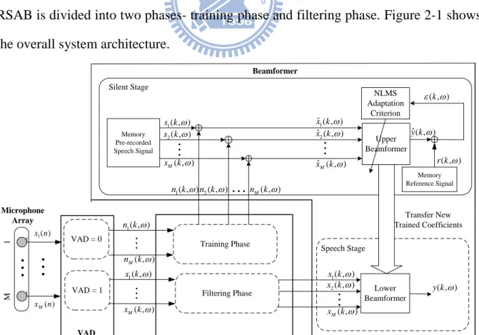
After collecting the pre-recorded signal and reference signal, the procedure of the RSAB is divided into two phases- training phase and filtering phase. Figure 2-1 shows the overall system architecture.

1 M ) (n xM VAD = 1 ) ( 1 n x



Microphone Array VAD = 0



VAD Training Phase Filtering Phase Beamformer 1( , ) x k   1( , ) x k ( , ) M x k Lower Beamformer Memory Pre-recorded Speech Signal



1( , ) s k 2( , ) s k ( , ) M s k Upper Beamformer Transfer New Trained Coefficients ( , ) y k ( , )k   ( , ) r k 1 ˆ ( , ) x k

-

Silent Stage Speech Stage



2 ˆ ( , ) x k ˆ ( , )M x k Memory Reference Signal 2( , ) x k



1( , ) n k n k2( , ) nM( , )k 1( , ) n k ( , ) M n k ( , ) M x k NLMS Adaptation Criterion ˆ( , ) y k

(17)

9

In the algorithm, the voice activity detection (VAD) is used to detect the activity of desired signal. When VAD shows that desired signal is inactive, the system started training phase using normalized least mean square (NLMS). For the training phase, the error signal at frequency  is written as





†

_ˆ

( , )

k

r k

( , )

( , ) ( , )

k

( , )

k

 







w



x





s



(2-5) where



1 2



( , )

k





w k

( , )



w k

( , )



w k

_M

( , )



T

w



1 2



ˆ

( , )

k





x k

ˆ

( , )



x k

ˆ

( , )



x

ˆ

_M

( , )

k



T

x



1 2



( , )

k





s k

( , )



s k

( , )



s

_M

( , )

k



T

s

and † denotes complex conjugate transpose.

 

( , )k is error signal. r k( , )



is the pre-recorded reference signal. w( , )k



is the filter weighting for adaption. xˆ( , )k



is the received signal from microphone array in training phase. And s( , )k



is pre-recorded desire source.

The purpose of RSAB is to minimize the mean square error between received signal and the desired signal. The mean square error is

( , ) ( , ) LMS

J 



 k

  

k _.

Then minimize the mean square error

† † min min ( , ) ( , ) ˆ ˆ min ( , ) ( , ) ( , ) ( , ) ( , ) ( , ) LMS J k k r k l k k r k l k k                 _  _{ }  _ W W W w x w x (2-6) The optimal solution would be obtained by taking the derivative to previous equation to find a local minimum. But the optimal solution is not practical for implementation. Therefore, the adaptive solution is introduced. For adaptive solution, the weighting

(18)

10 ( , )k



w is updated in the steepest direction thus

(_k1, )



 ( , )_k

 

 JLMS     w w w _. (2-7)

From (2-6) and (2-7) , using NLMS algorithm to achieve a stable solution in each frequency. Therefore, the filter weighting update procedure is

† ˆ ( , ) ( , ) ( 1, ) ( , ) ˆ ( , ) ( , )ˆ k k k k k k

 



 





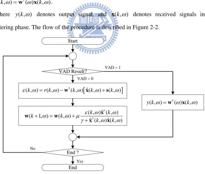
     x w w x x . (2-8)

When VAD detected that the received sound signal contains desired speech signal, the system switched to the filtering phase. The system starts to filter the received signal with w trained in training phase so

†

( , ) ( ) ( , )

y k  w  x k  .

Where y k( , ) denotes output signal, and x( , )k  denotes received signals in filtering phase. The flow of the procedure is described in Figure 2-2.

End ?

End

Yes VAD = 0

VAD Result? VAD = 1





† _ˆ ( , )k r k( , ) ( , )k ( , )k ( , )k     w  x  s  † ˆ ( , ) ( , ) ( 1, ) ( , ) ˆ ( , ) ( , )ˆ k k k k k k               x w w x x † ( , ) ( ) ( , ) y k  w  x k  No Start

(19)

11

Chapter 3 Linear Constrained Minimum Variance Beamforming

3.1 Introduction

Frost [7] proposed a method to minimize the target signal power under constraint. Griffiths and Jim [8] reconsidered the Frost’s algorithm and obtained generalized sidelobe canceler (GSC). GSC is widely used to cope with interference signal. Gannot

et al. [4] applied relative transfer function (RTF) to GSC to enhance the performance

when there’s a nonstationary desired source in a reverberant room. In this chapter the Frost algorithm is introduced and then RTF GSC.

3.2 Frequency Domain Frost Algorithm

3.2.1 Optimal Solution

Starting from the same problem formulated in section 2.2. The purpose is to find a set of weighting that filter the received signal and obtain the original desired source. The filter weighting in vector form is



1 2



( , )

k





w k

( , )



w k

( , )



w k

_M

( , )



T

w

.

The set of filter weighting can be used to filter the received signal so the output would be † † † ( , ) ( , ) ( , ) ( , ) ( , ) ( , ) ( , ) ( , ) ( , ) ( , ). s n y k k k k k s k k k y k y k



    w x w a w n (2-1)

(20)

12

andy kn( , ) denotes interfering part of filtered signal. The output power would be



 

† †



† ( , ) ( , ) ( , ) ( , ) ( , ) ( , ) ( , ) ( , ) ( , ) E y k y k E k k k k k k k



 _  _xx w x x w w w (2-2)

where xx( , )k  denotes power spectral density of input signal. The goal is to

minimize output power. If there’s no constraint for the problem, the trivial solution would be zero. Therefore, a constraint is set as

† ( , ) ( , ) ( ) ( , ) ( , ) ( , ) D s y k k s k f k s k          w a (2-3)

where f( , )k  is a prescribed filter, usually let it a delay. Therefore, the linear constrained minimum variance (LCMV) problem can be formulated as:



†



†

min ( , )k



_xx( , ) ( , ) subject to k



k



( , ) ( )k

 

 f( , )k



w w w w a (2-4)

Using complex Lagrange multipliers to solve the problem

† † † ( ) ( , ) ( , ) ( , ) ( , ) ( ) ( , ) ( ) ( , ) ( , ) k k k k c k k c k                   _  _    _  _ xx w w w w a a w

where  is the Lagrange multiplier. Set the derivative of ( )w with respect to w

to be zero yields ( ) ( , ) ( , )k  k   ( ) 0  _{ } _ _  xx w w a w (2-5)

By (2-3) and (2-5) , the optimal solution of LCMV problem would be

1

† 1 1

( , )k  _ ( ) _xx ( , ) ( )k   _ _xx ( , ) ( ) ( , )k   f k 

w a a a (2-6)

3.2.2 Adaptive Solution

The constrained form of the optimal solution is impractical in the real world. It’s difficult to find the room impulse response by using system identification method. This constrained form can’t tract changes in the environment [4]. So by Frost [7], the

(21)

13

adaptive form was introduced, which would be more useful in practical environment. Consider the steepest descent adaptive algorithm:





( ) ( 1, ) ( , ) ( , ) ( , ) ( , ) ( ) . L k k k k k                 _xx  w w w w w w a (2-7)

Imposing the constraint on w(k1, )



. Then

† † † † ( ) ( ) ( 1, ) ( ) ( , ) ( ) ( , ) ( , ) ( ) ( ) D D D D D f k k k k                  _xx  a w a w a w a a _.

Solving the Lagrange multiplier yields

(k1, )  ( ) ( , ) k    ( )_xx( , ) ( , )k  k   ( ) w P w P w f (2-8) Where † † 2 ( ) ( ) ( ) ( ( )) ( ) D D D D       a a  P I a a (2-9) † 2 ( ) ( ) ( ) ( ( )) ( ) D D D f       a  f a a (2-10) ( )



P is the projection matrix that project vector to the null space of aD†( ) . And

†

(aD ( )) represents the null space of aD†( ) .f( )



is the range space of aD†( )

and



aD†( )



represents the range space of aD†( ) . From (2-2), replacing ( , )k 

_xx by E



x( , )k  x†( , )k 



and rearrange (2-7), the adaptive Frost algorithm would be

(k1, )  ( ) _ ( , )k   ( , ) ( , )k  y k  _ ( )

(22)

14

3.3 Generalized Sidelobe Canceler

From the frost algorithm, the filter weighting could be separated into two parts; the first part is the range space of aD( ) and the second part is the null space of

( ) D  a . Hence FBF ANC ( , )k   ( , )k   ( , )k  w w w (2-12) where † FBF( , ) ( ( )) D k    w a and w_ANC( , )k   (aD†( ))

comparing the filter weighting with adaptive Frost algorithm, let

FBF 2 ( ) ( , ) ( ) ( ) ( ) D D k    f     a w f a (2-13) and ANC( , )k   ( ) ( , ) k  w P g . (2-14)

From (2-12), (2-13) and (2-14),the output signal would be

† † † FBF NC † † † FBF ANC ( , ) ( , ) ( , ) ( , ) ( , ) ( , ) ( , ) ( ) ( , ) ( , ) ( ) ( , ) ( , ) ( , ) y k k k k k k k k k k y k y k                     w x w x w x f x g P x (2-15)

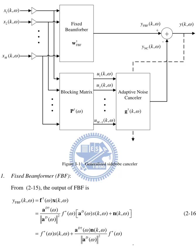
The architecture of GSC could be separated into three parts, fixed beamformer (FBF), blocking matrix (BM) and adaptive noise canceler (ANC). The purpose of FBF is to obtain the signal that contains the desired source and a stationary noise. The BM blocks the desired source to extract the stationary noise. Then the ANC uses multichannel wiener filter to estimate the noise of FBF and cancel the noise. Figure 3-1 shows the entire architecture of GSC. Detail discussion on each element in the architecture is given as follows.

(23)

15

Fixed Beamforber

Blocking Matrix Adaptive Noise

Canceler † FBF w † ( ) P g†( , )k 

+

FBF( , ) y k  NC( , ) y k  ( , ) y k  + -․ ․ ․ ․ ․ ․ ․ ․ ․ 1( , ) x k  2( , ) x k  ( , ) M x k  1( , ) M u _ k  1( , ) u k  2( , ) u k 

Figure 3-1 Generalized sidelobe canceler 1. Fixed Beamformer (FBF):

From (2-15), the output of FBF is

† FBF † 2 † 2 ( , ) ( ) ( , ) ( ) ( ) ( ) ( , ) ( , ) ( ) ( ) ( , ) ( ) ( , ) ( ) ( ) D D D D D y k k f s k k k f s k f     _ _ _ _               _  _   f x a a n a a n a . (2-16)

Because f( ) is just a simple delay, the output of FBF contains undistorted desired source and noise. This is an optimal solution where the desired source is just a simple delay from output of FBF. The issue of the optimal solution is that the actual TFs are difficult to find so Gannot et al. applied relative transfer function (RTF) to GSC to approach the suboptimal solution [4]. The RTF is easy to obtained by system

(24)

16

identification method proposed by [12]. RTF is the ratio of RIR between two microphones. Let the first microphone be the reference microphone then the RTF is





1 ( ) , 1, , ( ) m m D D D a h k m M a      . (2-17)

Take the vector form

 

1 1 ( ) ) 1 ( T D D M D D T D h h a



  _ _ a h

If the actual TFs in (2-13) are replaced by RTFs, the FBF would be

FBF 2 ( ) ( , ) ( ) ( ) D D k   f    h w h _. (2-18)

By (2-15) and (2-18) ,the output of FBF would be

FBF † 1 FBF † 2 † 2 ( , ) ( ) ( , ) ( ) ( ) ( ) ( , ) ( ( , ) ( ) ( ) ( , ) ( ) ( , ) ( ) ( ) ) D D D D D y k k f s k a k k f s k f     _ _ _ _                _  _   w x h a n h a n a (2-19)

Therefore, a suboptimal solution is obtained with signal distorted by the transfer function of desired source to the first microphone.

2. Blocking Matrix(BM):

The BM using RTFs could properly block the desired signal. Therefore, the columns of BM are the bases of desired signal null space. Therefore, considering the following matrix

(25)

17 3 2 1 1 1 1 0 ( ) ( ) ( ) ( ) ( ) ( ) 0 ( ) 0 1 0 0 0 1 M a a a a a a                                       P . Then the output of BM is

1 1 1 1 1 1 1 ( , ) ( , ) ( , ) ( ) ( , ) ( ) ( ) ( , ) ( ) ( ) ( ) ( ) ( ) ( ) 1, , 1. ( ) ( ) = ( ) m m m m m D D D D D D D m m m D D D u k x k x k a s k n a a a a a s k n n a a n m M                              (2-20)

Therefore, output of BM would be the noise only signal.

From the criterion of GSC, the output of blocking matrix should be independent of k because the noise is assumed stationary. But in practical, the BM cannot block the entire desired signal. Thus the output of BM would be changed under nonstationary source. Thus the vector form of output from BM is





† † † ( , ) ( ) ( , ) ( ) ( ) ( , ) ( , ) ( ) ( , ). k k s k k k              u P x P a n P n (2-21)

3. Adaptive noise canceler (ANC):

The output of ANC would be noise only signal because P†( ) is the null space of desired signal. Thus by (2-15) and (2-21), the output of ANC is





† ANC † † † † † † ( , ) ( , ) ( , ) ( , ) ( ) ( , ) ( , ) ( ) ( ) ( , ) ( , ) ( , ) ( ) ( , ) y k k k k k k s k k k k                    g u g P x g P a n g P n (2-22)

(26)

18



_† 2



FBF( , ) ( , ) ( , )

E y k



g k



u k



Then the multichannel Wiener filter would be

1 ( ,k ) _uu ( ,k )_u_y( ,k ) g (2-23) where



†



( , )k  E ( , )k  ( , )k  _uu  u u



FBF



( , ) ( , ) ( , ) . y k  E k  y k   _u  u

To track the change of environment and achieve a stable solution, Gannot et al. use NLMS algorithm to recursively update the weighting of ANC [4], thus the weighting of ANC would be ( , ) ( , ) ( 1, ) ( , ) 1, , 1 ( , ) m m m est u k y k g k g k m M P k             . (2-24) By [4], let





2 ( , ) ( 1, ) 1 ( , ) est est m P k







P k



 





x k



(2-25)

where



is a forgetting factor. P_est( , )k  can be u†( , ) ( , )k  u k  , which also normalize the power and make the recursion more stable.

(27)

19

Chapter 4 Nullforming

4.1 Introduction

In this chapter, several methods are introduced to achieve nullforming and the associated algorithms are explained for the adaptive filters to enhance the desired source.

4.2 Differential Microphone

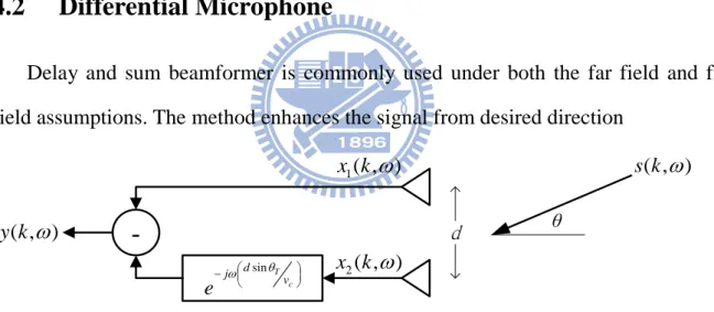
Delay and sum beamformer is commonly used under both the far field and free field assumptions. The method enhances the signal from desired direction

-sin T c d j v e     _ _ ( , ) y k  θ ( , ) s k  1( , ) x k  2( , ) x k  d

Figure 4-1 Differential microphone

Elko et al. [13] proposed differential microphone to reduce the signal from target direction. Figure 4-1 shows the architecture of differential microphone. The method makes a nullforming using two microphones subtraction with delay compensation. The signal is assumed a far field plain wave and the microphones are perfectly matched thus the output of differential microphone pairs can be written as,

(28)

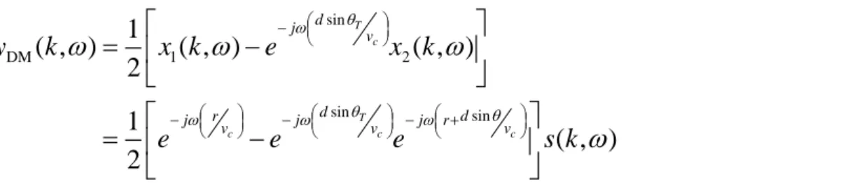
20 sin DM 1 2 sin _sin 1 ( , ) ( , ) ( , ) 2 1 ( , ) 2 T c T c c c d j v d _d r j j j r v v v y k x k e x k e e e s k    _           _ _        _ _  _ _  _  _    _  _      _  _   (3-1)

where y_DM( , )k  is the output of differential microphone pairs, s k( , )



is the source, d is the distance between two microphones, r is the distance between source and microphones, v_c is the speed of sound, θ is the direction of source, θ is the target direction of differential microphone, x k₁( ,) and x k₂( , ) are signals received by microphones. Rearrange the formula, the magnitude of output would be

 





sin 1 2 sin sin 1 ( , ) ( , ) ( , ) 2 1 1 ( , ) 2

sin sin sin ( , )

2 T c T c c d j _v DM d r j j _v v T c y k x k e x k e e s k d s k v            _ _ _    _ _      _  _ _ _ _        _  _   (3-2)

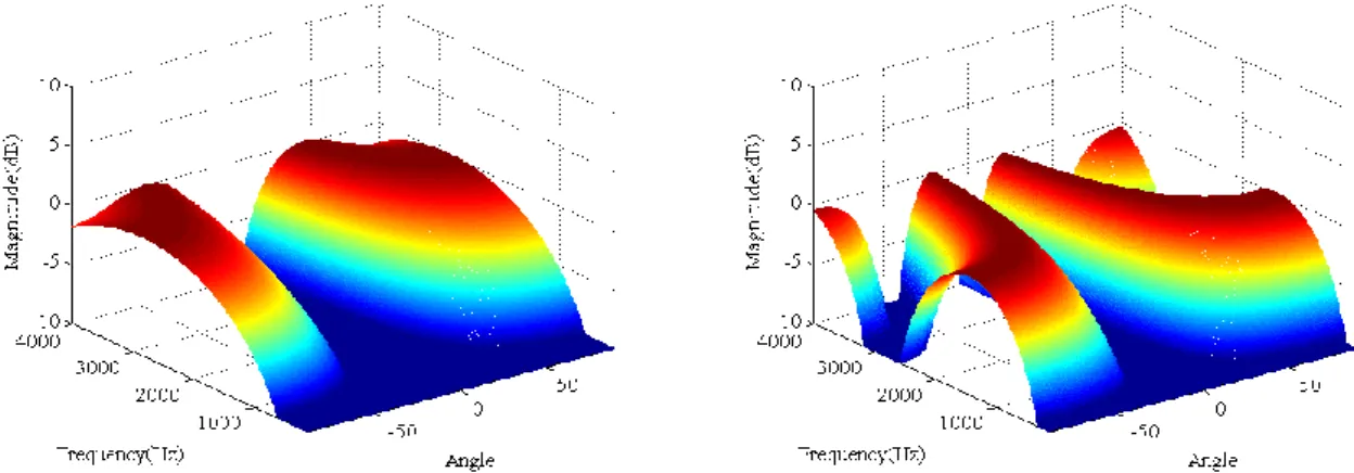
Figure 4-2 shows the beam patterns of differential microphone plotted by using equation (3-2). The beam patterns are plotted under different distance of microphones by letting the magnitude of source be 1, the speed of sound be 343 m/s and the target direction be .

The differential microphone works like high pass filter so differential microphone would enhance the noises in high frequencies. Different distance of microphones would affect the ability to deal with different frequency band. For the short distance differential microphone, lower band of frequencies would be eliminated from almost every direction.

(29)

21

Figure 4-2 Beam pattern of differential microphone with d=0.12 m (left) and d=0.24 m (right)

4.3 Nullforming Using Null Space of Interfering Signal

Previous section shows a nullformer for one interfering source. There may be two or more interfering sources in practical environment. The thesis uses singular value decomposition (SVD) to find the null space of the entire interfering signal. Assume there are N interfering sources in the environment and we have the RTFs of them as described by (2-17) in chapter 3. The RTFs of interfering sources are

2 1 ( ) 1 ( ) ( ( ) 1, , ( ) ) T IT I I i i iM I i I i h h i N a        _ _   h a

and take the complex conjugate of these RTFs in matrix form

1 2 ( ) ( ) ( ) ( ) I I I I N  _       _    H h h h

which are the bases of interfering signal subspace. Then applying singular value decomposition (SVD) toHI( ) † ( ) ( ) ( ) ( ) I      H U S V _(3-3) Where



1 2



( )



 ( )



( )



_M(



) U u u u

(30)

22



1 2



( )



 ( )



( )



_N( )



V v v v

are the eigenvectors of HI†( ) HI( )

1 2 ( ) ( ) ( ) ( ) 0 0 0 0 0 0 M                     S

are the singular values. These singular values are eigenvalues of HI†( ) HI( ) and

†

( ) ( )

I  I 

H H . From [14], the zero eigenvectors of HI†( ) HI( ) corresponds to the zero singular values

( ) 0, ( ) 0 1, , i  i  i N M   v     . ( ) i 

u corresponds to zero singular value for iN 1, ,M thus

†

( ) ( )

( ) (

)

0 1,

,

I i



i i

i

N

M









  

H

u

v

.

Therefore, u_i( ) are the null space bases of H( ) † for iN 1, ,M, That is

 

21 1 † 1 2 2 1 2 11 ( ) ( ) ( ( ) ( ) ( ) ( ) ( ) ( ) 1, ) , ( ) N T I I I N T I i i I I I N i I N a a a i N M                                H u u a a a u 0 h h h

Where 0



0 0



Tis a zero vector. Therefore,



1 ( ) 2 ( ) ( )



( ) I I I 1, , i    N  i N M    _    u a a a

This null space is a fixed nullformer where



1 2



( ) ( ) ( ) ( )

FN



 N



N



M



U u u u (3-4)

is an M input and N output filter.

(31)

23

4.4 Reference Signal Based Adaptive Filter with Fixed Nullforming

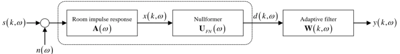
The nullformer could be used to block the interfering signals thus applying the nullformer to RSAB would eliminate the residual noise and reconstruct the desired source. Figure 4-3 shows the architecture of adaptive filter with nullformer. The effect of adaptive filter with nullformer could be considered as the convolution of room impulse response and impulse response of nullformer system.

Room impulse response Nullformer Adaptive filter

  FN  U   A Wk,  ,  s k y k ,   n   ,  x k d k ,

Figure 4-3 System of RSAB with fixed nullformer

For the case with multiple interfering sources described in (2-3).Let the multiplication of RIR and nullformer be a new room impulse

†

( ) ( ) ( )

FN







R U A (3-5)

and the new input of adaptive filter would be





† † † † † 1 † † ( ) ( ) ( ) ( , ) ( ) ( ) ( ) ( ) ( ) ( , ) ( , ) ( , ) ( , ) ( , ) FN FN i FN FN FN FN FN N D D I I i i D D k k k s k s k s k                      _      



d U x U A s n U a U a U n U a U n (3-6) where



1 2



( , )k   d k( , ) d k( , ) d_{M N}_ ( , )k  T d (3-7)

is the output of nullformer. Therefore, the input of adaptive filter would be M-N channels.

The nullformr would cause a great distortion for it’s a high pass filter. Therefore, the reference signal of RSAB would be used to reconstruct the desired signal. In the

(32)

24

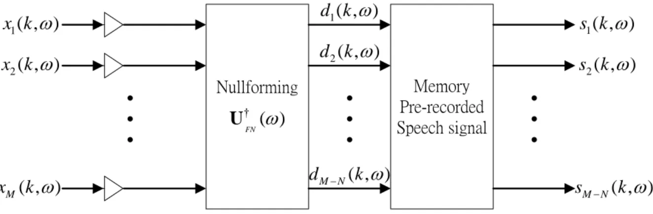
pre-recording procedure showed in Figure 4-4, the pre-recorded

signals-1( , ),..., M N( , )

s k  s _ k  are received by the output of nullformer and the reference signal-r k( , )



_{would be the desired signal with good quality.}

Nullforming Memory Pre-recorded Speech signal ․ ․ ․ 1( , ) x k  2( , ) x k  ( , ) M x k  ․ ․ ․ ․ ․ ․ † ( ) FN  U 1( , ) d k  2( , ) d k  ( , ) M N d _ k  1( , ) s k  2( , ) s k  ( , ) M N s  k  Figure 4-4 Pre-recording procedure of RSAB

The procedures of training phase and filtering phase are the same as described in section 2.3. The only difference is that there’s a nullformer before the input of adaptive filter. Figure 4-5 shows the architecture of RSAB.

Nullforming RSAB ․ ․ ․ 1( , ) x k  2( , ) x k  ( , ) M x k  ․ ․ ․ † ( ) FN  U 1( , ) d k  2( , ) d k  ( , ) M N d _ k  ( , ) y k  † ( ) w Desired signal

Figure 4-5 System architecture of RSAB

4.5 Generalized Sidelobe Canceler with Fixed Nullforming

Ordinary GSC does not work for the condition with nonstationary interfering signal in the environment. The existence of nonstationary signal does not satisfy the

(33)

25

criterion of GSC. The work in [10] proposed a dual-source transfer function GSC (DTF-GSC) method to eliminate a directional nonstationary source by modify the FBF and BM. DTF-GSC could block one nonstationary source. But when there are two or more interfering sources, DTF-GSC is not effective in blocking all these sources.

There are some features when applying the nullformer to GSC. Figure 4-2 shows that the nullformer is a high pass filter. The high pass feature would cause the received signal a great distortion. Therefore, the fixed beamformer and blocking matrix must be modified to satisfy the architecture of GSC with nullformer.

From (3-5), the effect of nullforming is the multiplication of RIR and impulse response of nullformer. Multiply the nullformer weighting from (3-8) with desired signal RTF. Then the new RTF is

† ) ( ) ( ) ( FN Null







D



h U h (3-9) Where 2 2 1 1 1 ( ) ( ) _{( )} ( ) 1 ( ) ( ) ( ) T D D _D D D D D a a a a a          _ _      a h

is the desired signal RTF and

1 2

( ) ( ) ( ) ( )

M N

T

Null Null Null Null

h h h

 _{ }   _  _

h

is the new RTF, which is the null space of interfering signals, from (3-4)

† † † † 1 1

( )

( ) 0

Null I D I FN









h

a

h

U

a

.

Apply SVD to the new obtained RTF

( ) ( ) ( ) ( ) Null     H  h (3-10) Where



1 2



( )  ( )  ( ) _{M N}_ ( ) T are the eigenvectors of hNull( ) hNull†( )

(34)

26 1 2 ( ) 0 0 0 ( ) ( ) 0 0 0 _{M N}( )          _        _   

are the singular values. These singular values are eigenvalues of hNull( ) hNull†( )

and hNull†( ) hNull( ) .

 



1( ) 2( ) ( )



T M N

       _ 

are the eigenvectors of hNull†( ) hNull( ) _{. The zero singular values correspond to zero}

eigenvectors so 1 1 † ( ) ( ) ( ) ( ) ( ) ( ) 2, , Null i i i i M N          _ _ _{ } _  h 0    . (3-11)

For ₁( ) is an 1×1 vector, let

1 1 1 ( ) ( ) ( ) ( ) n



  w





(3-12)

And multiply the RTF hNull†( ) with w_u( ) (3-13)

† † 1 1 1 † 1 ( ) ( ) ( ( ) ( ) ( ) 1 ( ) ( ) ( ) ( ) ( ) ) Null D FN D FN n D n a



     w w h h U a U





Thus 1 1 † 1 1 ( ) ( ) ( ) ( ( ) ( ) ) D FN D a



   a U





(3-14)

Therefore, the new FBF would be obtained

( ) _F ( ) ( )

NFBF   N  n 

w U w (3-15)

(35)

27 1 1 1 1 1 1 † FBF † 1 † † † † † † 1 † † 1 † 1 1 ( , ) ( ) ( , ) ( ) ( ) ( , ) ( ) ( ) ( , ) ( ) ( , ) ( ) ( ( ) ( ) ( ) ( ) ) ( ) ( ) ( , ) ( ) ( ) ( ) ( ) ( ) ( ) ( ) ) , ( FN FN FN NFBF u D D D N D I I i i i D FN D y k k k s a k s k s k s k                                     _   _     _ _       



w x w x a a n n U U a U U       1 1 1 † † † ( ) ( ) ( ) ( ) ( ) FN          U n  (3-16)

The FBF would block the interfering signal and make a beam to the desired signal. Let



2 2 1



( ) ( ) ( ) ( )

n







M N 



P



. The blocking matrix would be

( ) ( ) ( )

NBM   FN  n 

P U P (3-17)

Then the output of BM is

† † † 1 † † † † 2 1 † † † † † † † † ( , ) ( ) ( , ) ( ) ( ) ( ) ( , ) ( ) ( , ) ( ) ( ) ( ) ( ) ( , ) ( ) ( ) ( ) ( ) ( ) ( , ) ( ) ( ) ( ) ( ) ( ( ) ) ( ) NBM FN FN FN FN N D I I n i i i D n D FN FN M D D D D N n n k k s k s k s k s k                                   _   _      _  _       



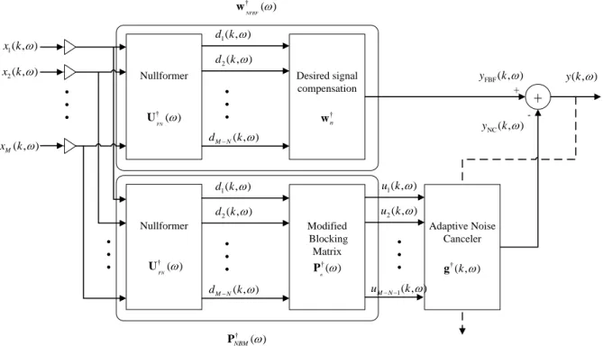
u P x P a a n P a n U U a U P U P U n a U   ( ) n (3-18) where



1 2 1



( , )k



 u k( , )



u k( , )



u_{M N}_{ } ( , )k



u

Therefore, the BM can block the desired signal and interfering signal and obtain the stationary noise. The ANC can be used to eliminate the residual stationary noise. Recalling section 3.3, the ANC is the same one as described in (2-24). The architecture of GSC with nullforming is showed in Figure 4-6.

(36)

28 Desired signal compensation Modified Blocking Matrix Adaptive Noise Canceler † n w † ( ) NBM  P †_{( , )}_k_ g + FBF( , ) y k NC( , ) y k ( , ) y k + -․ ․ ․ ․ ․ ․ 1( , ) x k 2( , ) x k ( , ) M x k 1( , ) M N u   k 1( , ) u k 2( , ) u k Nullformer ( , ) M N d _ k 1( , ) d k 2( , ) d k ․ ․ ․ ․ ․ ․ † ( ) FN  U Nullformer † ( ) FN  U ( , ) M N d _ k 1( , ) d k 2( , ) d k ․ ․ ․ ․ ․ ․ † ( ) NFBF  w †_{( )} n  P

(37)

29

Chapter 5 Variable Nullforming Adaptive Filter

5.1 Introduction

In previous chapters, several methods to approach nullforming are introduced. These nullforming methods are fixed so they are not able to track the interfering sources. For example, the weighting of nullformer was previously set to one desired direction so the nullformer works well when interfering sources emit in the exact direction. When there are new interfering sources from other direction or the original interfering source change the direction, these kinds of fixed nullformer are unable to block the interfering sources.

In this chapter, a novel method to construct a variable nullformer is proposed. The nullforming algorithm could trace the change of sources. Then the algorithm applies the variable nullforming to generalized sidelobe canceler to obtain the reconstructed desired signal.

5.2 Variable Nullforming

5.2.1 Estimate Signal Subspace Using Order Recursive Least Square

Starting from the estimation of RTF vector, the estimation of RTF vector is from the output of blocking matrix [4]. Blocking matrix contains the bases spanning the null space of RTF vector. When there’s only one sound source in action, rearranging the term (2-20) in chapter 3, the signal received from microphones are





1 1

( , ) _m , ( , ) ( , )

m m

(38)

30

Assume that the statistics of desired signal is stationary in each frame and the RIR changes slowly in a short period. Considering the cross PSD of kth frame

        1 1 1 1 ( ) 1 ( ) Φ , , Φ , Φ , 1, , m m t t x x k  hm k  x x k   u x k  t K (4-2)

where K is the number of frames for estimating RTFs. n km( , ),  m1,...,M are assumed stationary, s k( , )



and u k_m( , ) are independent thus





1

Φ ,

m

u x k  is

independent of the frame index k. [12] proposed a system identification method with nonstationary signal by applying least square (LS) estimation to the following equation













































1 1 1 1 1 1 1 1 1 1 (1) (1) ₍₁₎ (2) (2) (2) 1 ( ) ( ) ( ) Φ , 1 Φ , _, Φ , Φ , 1 Φ , , , , 1 Φ , Φ , m m m m x x x x _m u x x x x x m m K K K m x x x x k k _k k k k k h k k k k   _             _ _     _ _     _  __ _      _ _ _ _       _ _   _ _ _ _   . (4-3)

The RTFs are estimated when there’s only one source. When there is more than one source in the environment, the method could not describe the RTF properly. The work in [10] proposed a method to estimate the blocking matrix when there are two sources emitting simultaneously in the environment. When number of sources increases, the number of reference microphones increases. Increasing number of reference microphones would increase the number of nullforming directions. Considering N sources emitting simultaneously, the linear equation would become

































































1 1 1 1 2 1 1 1 1 1 1 1 1 2 1 1 2 1 1 (1) (1) (1) (1) 1 (2) (2) (2) (2) 2 ( ) ( ) ( ) ( ) Φ , Φ , 1 Φ , Φ , Φ , , Φ , 1 Φ , Φ , Φ , , Φ , 1 Φ , Φ , Φ , , m m N m N m N u x x x x x x x x m x x x x x x x x m K K K K N x x x x x x x x x m k k k k k h k k k k k h k k k k k h k                _            _                 













(1) (2) ( ) , , , m m K m k k k                                  (4-4)

多通道語音強化使用相對轉移函數建構之零波束形成

國 立 交 通 大 學

電控工程研究所

碩 士 論 文