支援RoF被動式光纖網路的動態頻寬分配

國 立 交 通 大 學

電信工程學系

碩 士 論 文

支援 RoF 被動式光纖網路的動態頻寬分配

Dynamic Bandwidth Allocations for Passive Optical Network

Supporting RoF System

研 究 生：黃禕達

指導教授：田伯隆 教授

支援 RoF 被動式光纖網路的動態頻寬分配

Dynamic Bandwidth Allocations for Passive Optical Network

Supporting RoF System

研 究 生：黃禕達 Student：Yi-Da Huang 指導教授：田伯隆 Advisor：Po-Lung Tien 國 立 交 通 大 學 電 信 工 程 學 系 碩 士 論 文 A Thesis

Submitted to Department of Communication Engineering College of Electrical and Computer Engineer

National Chiao Tung University in partial Fulfillment of the Requirements

for the Degree of Master of Science in Communication Engineering

February 2010

Hsinchu, Taiwan, Republic of China

支援 RoF 被動式光纖網路的動態頻寬分配

學生：黃禕達 指導教授：田伯隆 國立交通大學電信工程學系碩士班 摘 要 光纖和無線混合接取網路是一種新的接取網路。和光纖接取網路相 比，它可以解決光纖接取網路中最後一哩的問題。和無線接取網路相比， 它可以解決無線接取網路中通訊範圍不夠大和頻寬不夠的問題。本文的研 究是在討論一種混合接取網路中光纖網路部份的頻寬分配問題，因為光纖 網路在頻寬分配方面會受到無線網路的影響，所以提出兩個不同的動態頻 寬分配演算法來減低受到的影響，第一個演算法的目標是提高系統使用 率。第二個演算法的目標是在滿足高優先性流量服務品質的條件下，改善 低優先性流量的品質。

Dynamic Bandwidth Allocations for Passive Optical Network

Supporting RoF System

student：Yi-Da Huang advisor：DR. Po-Lung Tien

Department of Communication Engineering National Chiao Tung University

ABSTRACT

Optical and wireless hybrid access network is an integrated access network. Compared with optical access network, it can solve the “last mile” problem in optical access network. Compared with wireless access network, it can solve the problem of shortage of communication range and bandwidth in wireless access network. This study is to discuss bandwidth allocation problem in optical network of hybrid access network. Because optical network in the bandwidth allocation will be the impact of wireless network, propose two different dynamic bandwidth allocation algorithms to reduce the impact. The first algorithm aims to improve the system utilization. The second algorithm aims to improve quality of low priority traffic on the premise that high priority traffic quality-of-service can be maintained.

誌 謝

感謝我的指導教授田伯隆老師在這 2 年半的親切指導，在我迷失研究 方向時，老師會幫忙我，給我正確的研究方向。在我陷入低潮時，老師也 會伸出援手，使我可以突破困境。我可以產生出這篇論文，真的謝謝老師 的幫忙。 再來感謝啟賢學長、恭立學長、逸旻、偉民、柏宇平時在研究課題上 的討論，最後要感謝我的父母在背後支持我，給我關心和經濟上的支助， 使我可以專心的完成我的學業。

目

錄

中文摘要 ... i 英文摘要 ...ii 誌謝 ...iii 目錄 ... iv 圖目錄 ... v 表目錄 ...vii 1 Introduction ... 1 2 Background ... 4 2.1 Transmission in TDM PON... 4

2.2 EPON dynamic bandwidth allocation research... 6

2.3 Introduction of WiMAX... 7

2.4 Integration of EPON and WiMAX architectures ... 8

3 Proposed DBAs ... 10

3.1 Radio-over-fiber access network architecture... 10

3.2 Pursuing utilization algorithm ... 12

3.2.1 Weighted dynamic bandwidth allocation………..13

3.2.2 Remaining bandwidth allocation……….. 15

3.3 Enhanced DBA... 17

3.3.1 Enhanced DBA step1... 18

3.3.2 Enhanced DBA step2... 20

3.3.3 Enhanced DBA step3... 22

3.3.4 Enhanced DBA step4... 25

4 Simulation Results and Analysis ... 27

4.1 Pursuing utilization DBA results and analysis ... 30

4.2 Enhanced DBA results and analysis... 32

4.2.1 Results of enhanced DBA with different thresholds and analysis ... 32

4.2.2 Results of enhanced DBA with different delay bounds and analysis ... 36

4.2.3 Results of enhanced DBA with different burstinesses and analysis ... 38

5 Conclusions ... 42

圖目錄

圖 2-1. PON 架構... 4 圖 2-2. PON 架構中，TDMA 的下傳方式... 5 圖 2-3. PON 架構中，TDMA 的上傳方式... 5 圖 2-4. WiMAX 中 TDD 和 FDD 的傳輸方式 ... 8 圖 2-5. Independent architecture... 9 圖 2-6. Hybrid architecture ... 9

圖 3-1. Radio-over-fiber access network architecture ... 10

圖 3-2. Radio-over-fiber access network architecture 中的傳輸方式 ... 12

圖 3-3.表示 waiting time 的圖形 ... 13

圖 3-4. High priority pakcet 分類 ... 20

圖 3-5. Low priority pakcet 分類... 20

圖 3-6. Enhanced DBA step2 舉例 ... 22

圖 3-7. 加上可調參數調整給 high priority traffic 的 bandwidth... 23

圖 3-8. 調整參數 A 的流程圖... 25

圖 4-1. Two state bursty traffic model ... 29

圖 4-2. 不同 remaining bandwidth allocation 的比較 ... 30

圖 4-3. Proposed remaining bandwidth allocation 和 dividing remaining bandwidth 在不同 cycle length 的 average delay 比較 ... 31

圖 4-4. Enhanced DBA 在不同 threshold 的 packet out-bound rate ... 32

圖 4-5. Enhanced DBA 在不同 threshold 的 average delay， 以及和 strict priorityalgorithm 的比較 ... 33

圖 4-6. Enhanced DBA 在不同 threshold 的 variation，以及 和 strict priorityalgorithm 的比較 ... 33

圖 4-7. Enhanced DBA 在不同 delay bound 的 packet out-bound rate... 36

圖 4-8. Enhanced DBA 在不同 delay bound 的 average delay， 以及和 strict priority algorithm 的比較 ... 37

圖 4-9. Enhanced DBA 在不同 delay bound 的 variation， 以及和 strict priorityalgorithm 的比較 ... 37

圖 4-10. Enhanced DBA 在不同 burstiness 的 packet out-bound rate... 39

以及和 strict priority algorithm 的比較 ... 39 圖 4-12. Enhanced DBA 在不同 burstiness 的 variation，

以及和 strict priority algorithm 的比較 ... 40

表目錄

1 Introduction

隨著各式各樣寬頻接取網路技術的突破，在不久的未來無線網路將可 以提供定點 1Gbps 以及移動 100Mbps 的頻寬，有線網路像是 VDSL2、PLC 也可以提供 100Mbps 的頻寬。要將如此大量的資料連結上骨幹網路，目前 只有光纖能提供如此大量的頻寬，可以將多個無線以及有線的寬頻接取網 路同時穩定的連結上骨幹網路，因此有人就想出整合光纖接取網路和無線 接取網路的網路架構，使光纖接取網路和無線接取網路可以同時連結上骨 幹網路。在這篇論文中，就是在整合光纖接取網路和無線接取網路的網路 架構上提出動態頻寬分配，在這個整合網路中，整合的光纖接取網路是乙 太被動光纖網路(Ethernet Passive Optical Network) [1]，整合的無線接取網路 是 WiMAX(Worldwide Interoperability for Microwave Access)[2]。

在說明 EPON 前，先介紹 PON(passive optical network)，PON 是一種光 纖接取網路架構，整個架構包含 OLT(optical line terminal)、ONU(optical network unit)、splitter 和 cable。OLT 連接光纖接取網路和骨幹網路，主要 功能是分配頻寬和傳送或接收資料。ONU 連接光纖接取網路和 end user， 它負責將從 OLT 下傳的 packet 轉換成不同的介面傳送給 end user，同時負 責將 end user 上傳的資料傳送給 OLT。PON 是 point-to-multipoint 的 optical network，訊號從起點到終點的路徑中，都沒有使用主動元件，也就是說在 OLT 和 ONU 之間的所有元件都是屬於不需要額外提供電源即可動作的被動

元件，因此被稱為被動光纖接取網路。這種接取網路的最大好處是在架設 網路時不需要考慮複雜的電源問題，同時容易維護。EPON 是 PON 的一種， 它是將資料包裝成 Ethernet frame 來傳輸，所以可以支援 Ethernet network。 因為 Ethernet network 是最普及的 local area network，所以 EPON 網路是建 置光纖網路的首選。WiMAX 網路是一種點對多點的無線接取網路，和其它 無線網路相比，它可以提供較大的頻寬，較廣的通訊覆蓋範圍，並提供服 務品質保證。

此篇論文研究的 EPON 和 WiMAX 整合網路架構是在 central office 將 OLT 和 BS(base station)整合在一起，ONU 會加上 remote antenna unit，用來 接收或發射無線訊號，在 ONU 端會直接將收到的無線 RF 訊號直接調變成 光訊號送入光纖中，使無線訊號可以在光纖中傳送，避免無線訊號不同訊 號格式轉換，所以容易支援各種不同無線網路，同時無線訊號可以集中於 局端處理，遠端節點可以簡化架構，降低成本，但是這樣會有一個問題， 因為整個整合網路中只使用一個波長的 laser 作上傳，而上傳的無線 RF 訊 號在送到 ONU 端時，要直接上傳到光纖中，不會先存在 ONU 的 buffer， 所以無線訊號在上傳時，有線訊號就無法上傳，因此光纖網路在這個整合 架構中會受到無線網路很大的影響。針對這個問題，對光纖網路的頻寬分 配提出兩個不同的 dynamic bandwidth allocation，來改善無線網路對光纖網 路在頻寬分配上的影響。第一個 DBA 的目標是提高光纖網路的 system

utilization。第二個 DBA 的目標是 delay 超過 delay bound 的 high priority packet 佔全部 high priority packet 的比例小於 threshold 的條件下，改善 low priority traffic 的 average delay 和 jitter。

這篇論文之後的章節編排將如下，第二章介紹一些相關的背景知識； 第三章介紹本論文所研究的網路架構，並針對光纖接取網路在這個架構中 做頻寬分配所遇到的問題提出 DBA 來改善；第四章則是模擬環境的介紹及 模擬結果的分析比較；第五章是說明提出的 DBA 所達到的效果，並對未來 研究的方向做探討。

2 Background

2.1 Transmission in TDM PON

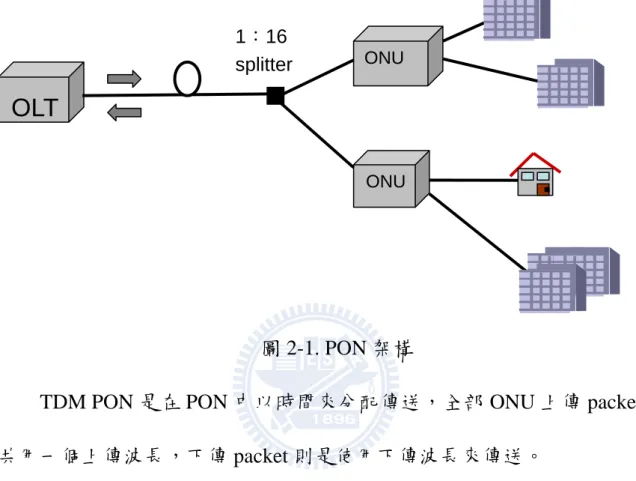
圖 2-1. PON 架構

TDM PON 是在 PON 中以時間來分配傳送，全部 ONU 上傳 packet 是 共用一個上傳波長，下傳 packet 則是使用下傳波長來傳送。

在下傳部份，採用 broadcast 的方式，packet 是由 OLT broadcast 出去， ONU 只會收下要送給自己的 packet，否則會忽略或是拒絕。在上傳部份， 採用 TDMA(time-division multiple-access)或 WDMA (wave-division

multiple-access)的方式，因為整個 PON 的上傳頻寬要給全部 ONU 使用，所 以要做頻寬分配，使 packet 不會發生 collide。

OLT

ONU 1：16 splitter ONU

圖 2-2. PON 架構中，TDMA 的下傳方式

圖 2-3. PON 架構中，TDMA 的上傳方式

IEEE 802.3ah 提出一種叫做 multipoint control protocol( MPCP)的機制來 解決頻寬分配的問題，每一個 ONU 會送 REPORT message 給 OLT，REPORT message 包含頻寬需求、buffer 剩多少容量等訊息來協助 OLT 分配頻寬。OLT 則會根據收到的 REPORT message 送 GATE message 給每一個 ONU，通知 每一個 ONU 在分配到的時間間隔傳送。

2.2 EPON dynamic bandwidth allocation research

本論文研究的網路是整合 EPON 和 WiMAX 的網路，主要研究的則是 整合網路中EPON的dynamic bandwidth allocation。在本節對一些已經提出的 EPON bandwidth allocation algorithm做介紹。在[3]和[4]中作者提出IPACT (interleaved polling with adaptive cycle time)，IPACT是ONU在收到GATE message後立刻上傳資料和REPORT給OLT，OLT根據RTT和request這些訊息 決定下個round ONU在哪些時間間隔可以上傳，但是這個方法無法提供QoS 給delay、jitter要求嚴格的traffic，因為IPACT中的cycle time是變動的。在[5] 一文中，作者提出稱為Estimation-Based DBA(EB-DBA)的方法，OLT決定要 給ONU多少transmission window是根據之前的queue length和grant length紀 錄，但無法準確的預測queue length。[6]和[7]提出的方法是IPACT with Grant Estimation (IPACT-GE)，是根據traffic的self-similarity性質預測在polling間隔 時間會來多少packet量，因為這個方法預測準確，所以可以對average delay 有改善。在[8]中作者提出TLBA (two-layer bandwidth allocation)，這個方法 包含class-layer分配和ONU-layer分配，class-layer分配是根據service class的 total request將全部頻寬分給3種不同的class，同時每種class根據weight可以 得到不同的保證頻寬。ONU-layer分配是每個class根據max-min fairness principle將得到的頻寬分給ONU。但這個方法不能根據traffic的QoS要求來 動態的改變class的weight，因此提出[9]再對TLBA作更深入的研究，提出一

個方法根據每個class的traffic load和access delay bound來動態改變class的 weight，使頻寬能被有效的利用，也就是要求QoS的class在QoS滿足的前提 下，能把多的頻寬給沒有QoS要求的class。

2.3 Introduction of WiMAX

WiMAX((Worldwide Interoperability for Microwave Access)，這個網路 所使用的傳輸協定是 IEEE 所制定的 802.16 standard，最初是在 2001 年所提 出，之後為了可以提供服務給移動式的使用者，在 2005 年訂出 IEEE 802.16e standard。目前也持續在對 IEEE 802.16 standard 提出補充或修改。

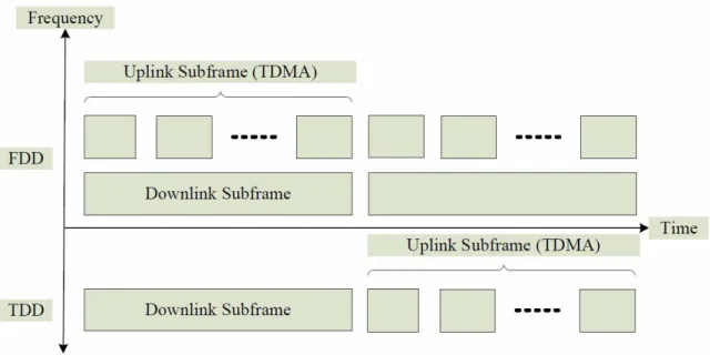
IEEE 802.16 standard 在 MAC 層的部份有提供 2 種傳輸方式。一種是 TDD，另一種是 FDD。如果是使用 TDD 來傳輸，則會將時間以固定的 frame 作分割，一個 frame 又可分為 uplink subframe 和 downlink subframe，在 uplink subframe 中頻寬就只能用來上傳，在 downlink subframe 中頻寬就只能用來 下傳。uplink subframe 和 downlink subframe subframe 的比例雖然能做調整， 但要調整的話，必須整個 WiMAX 網路的使用者都重新做同步，會影響很 大，所以通常會將這個比例固定。如果使用 FDD 來傳輸，則上傳和下傳可 以同時間進行，但上傳和下傳必須使用不同的頻帶。本篇論文所要整合的 無線網路就是以 TDD 方式傳輸的 WiMAX。圖 2-4 是表示 TDD 和 FDD 的 傳輸方式。

圖 2-4. WiMAX 中 TDD 和 FDD 的傳輸方式

2.4 Integration of EPON and WiMAX architectures

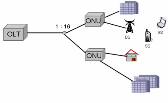
在[10 ]中提出幾種整合 EPON 網路和 WiMAX 網路的架構，以下將介紹其 中的 independent architecture 和 hybrid architecture。

A. independent architecture

在這個架構中，EPON 和 WiMAX 是 2 個獨立的網路，優點是整合簡單， 只要有共同的介面(e.g.,Ethernet)2 個網路就能連接起來，然而因為 2 個網路 彼此不能交換訊息，所以無法使整個系統做到理想的頻寬分配。

B. hybrid architecture

在這個架構中，ONU 和 WiMAX BS 整合成一個 system box，稱為 ONU-BS，因為 ONU-BS 能夠知道 2 個網路的 bandwidth request、packet scheduling 等訊息，所以比起 independent architecture，這個架構的 bandwidth allocation 會更有效率。

圖 2-5. Independent architecture

3 Proposed DBAs

3.1 Radio-over-fiber access network architecture

本論文研究的 dynamic bandwidth allocation algorithm 是在 radio-over- fiber architecture 下運作，這個架構如圖 3-1 所示。在這個架構中，是將 WiMAX 的 BS 整合到 OLT 中，而 ONU 會加上 antenna unit，antenna 收到 RF 訊號後，不會對訊號作解調，也不會存在 buffer，而是用直接調變光強 度的方式把訊號轉換成光訊號，使無線訊號在光纖中傳送。這個架構的優 點如下：(1)RF 無線訊號直接在光纖傳送，避免不同訊號格式轉換，容易支 援各種不同無線網路。(2)無線訊號集中於 central office 處理，遠端節點可 以簡化架構，降低成本。(3)藉由光纖延伸來解決無線傳輸死角。

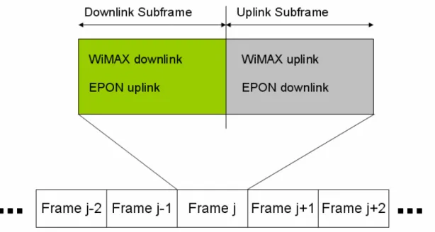
本論文要研究的網路是整合 EPON 和 WiMAX 的網路，在這個網路中 上下傳分別只使用一個波長。在整合的網路中，EPON 是使用 TDMA 的方 式傳送資料，WiMAX 是使用 TDD 的方式來傳送資料，在 uplink subframe 這段時間，因為 antenna 收到 RF 訊號後就要立刻轉成光訊號然後上傳到光 纖中，而且 EPON 和 WiMAX 這 2 個 network 共用一個上傳波長，所以頻 寬只能給 WiMAX 來上傳資料，EPON 只能下傳資料，不然 EPON 上傳的 資料會和 WiMAX 中上傳的資料發生碰撞。在 downlink subframe 這段時間， 因為 ONU 收到 BS 經由光纖下傳的光訊號後就要立刻轉成電訊號給 SS，而 且這 2 個 network 共用下傳波長，所以 WiMAX 只能下傳資料，EPON 只能 上傳資料。

因為 2 個網路在整合網路中的上下傳時間要分開，而且 TDD WiMAX 是以 uplink subframe 和 downlink subframe 來分割上傳和下傳的時間，所以 決定在 downlink subframe 這段時間中，WiMAX 只能下傳資料，EPON 只能 上傳資料，在 uplink subframe 這段時間中，WiMAX 只能上傳資料，EPON 只能下傳資料。Frame、uplink subframe 和 downlink subframe 的長度都是固 定的。Radio-over-fiber architecture 中 2 個網路的傳輸方式如圖 3-2 所示。

圖 3-2. Radio-over-fiber access network architecture 中的傳輸方式

3.2 Pursuing utilization algorithm

由於要避免 2 個網路的資料發生碰撞，所以使這 2 個網路上傳和下傳 的時間錯開，結果對 EPON 產生了一些 constraint。

第一個 constraint 是每個 round 中 OLT 所能分配的頻寬是固定，就算這 個 round 中要上傳的資料很少，也必須把頻寬用完，也就是說每個 cycle 的 時間都是固定的，沒辦法彈性的變化。

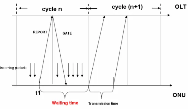
針對第一個 constraint，認為可以改善 system 的 utilization，也就是預測 waiting time( send REPORT 到下個 round 送 data 的間隔時間) 會來多少 packet，然後把多餘的頻寬分配給這些 packet，提出的 DBA 稱為 pursuing utilization DBA。Pursuing utilization DBA 是由 2 部份組成，分別是 weighted DBA[11]和 remaining bandwidth allocation，以下將分別介紹。

圖 3-3. 表示 waiting time 的圖形

3.2.1 Weighted dynamic bandwidth allocation

PON access network 有 N 個 ONU，PON 的 transmission speed 是 R bit/s， Tcycle 是全部 ONU 可以上傳的時間，Tg 是 guard time。

Step1：當 ONU 收到全部 ONU 傳來的 REPROT 後，首先算出每個 ONU 的 minimum guaranteed bandwidth。

：( Tcycle – 2 * N * Tg )* R / N (3.1) 因為 Ethernet traffic 的 bursty 性質，所以會發生一部份 ONU 的 request 較 少，而其它 ONU 的 request 大於 的情形。因此會產生 total excessive

bandwidth M

(

min r

)

i i i B −B

∑

( M 是

(

min r

)

i i B >B ONU 的集合 )。為了不浪費 total

excess bandwidth，於是提出一個方法來分配 bandwidth，這個方法就是 request 小於 minimum guaranteed bandwidth 的話，granted bandwidth 就是

min i B min i B

request，反之，granted bandwidth 就是 minimum guaranteed bandwidth 加上 excess bandwidth，excess bandwidth 是從 total excess bandwidth 分配出來， request 越大則可以得到越多 excess bandwidth，這個方法如(3.2-1)、(3.2-2) 所示。

(3.2-1)

(3.2-2)

：ONUi 的 request bandwidth ：OLT 給 ONUi 的 bandwidth ex

i

B

_{：分配給 ONUi 的 excess bandwidth}

Step2：經過第一次的分配後，可能會有 ONU 發生 grant length 大於

request 的情形，產生沒有使用到的頻寬( K

(

g r

)

j j j B −B

∑

，K 是

(

g r

)

j j B >B ONU 的集合 )，於是就依照 request 大小方法來分配這些多出來的頻寬，方法如 下所示： (3.3-1) (3.3-2)

Step3：如果頻寬還有剩而且有 ONU 是( > )，就重覆做 step2，直

到頻寬用完或全部 ONU 都是( ≤ )。

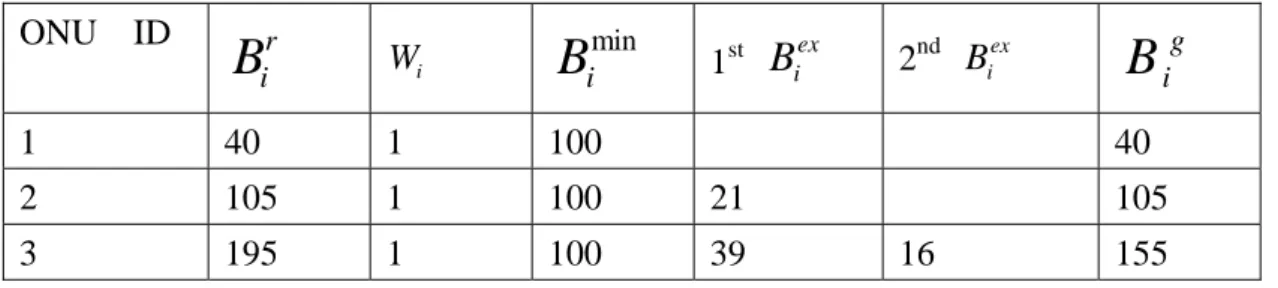
total bandwidth = 300bit ONU ID _r i

B

W i min i

B

1st B_iex 2nd B _iex g i

B

1 40 1 100 40 2 105 1 100 21 105 3 195 1 100 39 16 155

表 3-1.Weighted DBA example

表 3-1 是 weighted DBA 的舉例。假設 PON 中有 3 個 ONU，每個 cycle 可以分配的頻寬是 300 bit，每個 ONU 的 minimum guaranteed bandwidth 是 100 bit，每個 ONU 的 request 分別是 40 bit、105 bit 和 195 bit。在 step1 中， 因為 ONU1 的 request 小於 minimum guaranteed bandwidth，所以得到的頻寬 會和 request 一樣是 40 bit，而多出來的 60bit 頻寬會根據 request 大小分給 request 大於 minimum guaranteed bandwidth 的 ONU2 和 ONU3，因此 ONU2 得到 121 bit，ONU3 得到 139bit。因為 ONU2 的 request 是 105bit，會有 16bit 的頻寬多出來，所以執行 step2。因為只剩 ONU3 的 request 大於 granted bandwidth，所以把 16bit 都給它。最後 3 個 ONU 得到的頻寬分別是 40 bit、 105 bit 和 155 bit。

3.2.2 Remaining bandwidth allocation

在 radio-over-fiber 架構中，OLT 在每個 round 可以使用的頻寬是固定 r i B g i B r i B Big

的，所以做完 weighted DBA 後，可能會有剩下的頻寬，為了有效利用這些 剩餘頻寬，因此提出 remaining bandwidth allocation algorithm，這個 algorithm 的介紹如下。

預測 ONU 在 waiting time 會來多少 packet，根據預測來分配 remaining bandwidth。REPORT 除了有 buffer 訊息還有 traffic state 訊息。首先 OLT 根據 REPORT 傳來的 traffic state information，將 ONU 分為 2 類，traffic state 是 idle 的稱為 idle ONU，traffic state 是 bursty 的稱為 bursty ONU。

預測全部 bursty ONU 在 waiting time 中來的 packet 量，以 X 表示。預 測全部 idle ONU 在 waiting time 中來的 packet 量，以 Y 表示，根據 X 和 Y 的比例來分配 remaining bandwidth，使 waiting time 中來比較多 packet 的 ONU 可以得到較多的 remaining bandwidth。假設每個 ONU 的 waiting time 一樣。

X = λH * bursty onu number * waiting time (3.4-1) Y = λL * idle onu number * waiting time (3.4-2) λH：bursty state arrival rate

λL：idle state arrival rate

bursty onu number ：state 是 bursty 的 ONU 個數 idle onu number ：state 是 idle 的 ONU 個數

每個 bursty ONU 能拿到的 remaining bandwidth：

(3.5-1) 每個 idle ONU 能拿到的 remaining bandwidth：

(3.5-2)

ONU 最後能拿到的頻寬就是 weighted dynamic bandwidth algorithm 分 配的頻寬加上 remaining bandwidth allocation 所分配的頻寬。

3.3 Enhanced DBA

由於要避免 2 個網路的資料發生碰撞，所以使這 2 個網路上傳和下傳 的時間錯開，結果對 EPON 產生了一些 constraint。第二個 constraint 是 ONU 送出 REPORT 後到下個 round 可以送出 data 的時間變長，因為 ONU 在送 出 REPORT 後要等 WiMAX 的上傳時間結束才可以上傳。也就是說和原來 的 EPON 相比，ONU 送出 REPORT 後到下個 round 送出 data 的間隔時間多 了一個 uplink subframe 的時間。

因為 ONU 送出 REPORT 後到下個 round 可以送出 data 的時間變很長， 也就是說如果 bandwidth allocation algorithm 是 strict priority 的話，low priority traffic 的 delay 和 jitter 會比在 EPON 上差很多。而 enhanced DBA 的

目標是在滿足 high priority traffic QoS 的條件下，盡量給 low priority traffic 頻寬，所以一部份的 low priority packet 可以比較早送出去。因為 cycle 很長， 所以一部份的 low priority packet 可以比較早送出去的話，low priority traffic 的 performance 就可以有一定的改善，因此 enhanced DBA 和全部頻寬先分 給 high priority traffic 的 algorithm 相比，在滿足 high priority traffic QoS 的條 件下，能使 low priority traffic performance 有改善。

Enhanced DBA 所追求的 QoS 是 delay 超過 bound 的 high priority packet 佔全部 high priority packet 的比例要在 threshold 下，[12]和[13]是 delay 超過 bound 的 high priority packet 就會捨棄掉，追求的 QoS 是 high priority packet 捨棄的數目佔全部送出去的 high priority packet 的比例要在 threshold 下，類 似於 enhanced DBA 所追求的 QoS。[8]和[9]的目標也是在滿足 high priority traffic QoS 的條件下，盡量給 low priority traffic 頻寬，但這 2 個 algorithm 都不能控制 high priority traffic 的 QoS，也就是說會發生 high priority traffic 的 QoS 和 threshold 還有一段差距，還可以給 low priority traffic 一部份頻寬 時，但卻把全部頻寬給 high priority traffic。另外這 2 個 algorithm 也沒有使 high priority packet 一定可以比同時到達的 low priority packet 先送出去。以 下是 enhanced DBA 的敘述。

Step1 是 ONU 作 packet 分類。ONU 在要送 REPORT 給 OLT 時，會對 high priority packet 和 low priority packet 作分類。high priority packet 依照 bound time 作分類，low priority packet 依照 arrive time 作分類。

step1-1：假設目前時間是在 cycle n，delay bound 上限是 cycle k，根據 bound time 對 high priority packet 作分類。bound time 在 cycle (n + 1)之前的 全部 packet 量就稱為 high request[0]。bound time 在 cycle (n + 1)的全部 packet 量就稱為 high request[1]。在 cycle (n + 1)以後每個 cycle 平分成 M 等份， bound time 在 cycle (n + 2)第一部份的全部 packet 量就是 high request[2],1， bound time 在 cycle (n + 2)第二部份的全部 packet 量就是 high request[2],2， 依此類推，bound time 在 cycle (n + k)最後一部份的全部 packet 量就是 high request[k] , M。圖 3-4 是 high priority packet 分類的例子。

step1-2：也對 low priority packet 作分類，根據 packet 的 arrive time 來 分類，如果 packet 的 arrive time 小於或等於 high request[1]，則這些 packet 的總量稱為 low request[1]。如果 low priority packet 的 arrive time 和 high request[2],1 相同，則這些 packet 的總量稱為 low request[2],1。如果 packet 的 arrive time 和 high request[2],2 相同，則這些 packet 的總量稱為 low request[2],2，依此類推，如果 packet 的 arrive time 和 high request[k],M 相同， 則這些 packet 的總量是 low request[k],M。圖 3-5 是 low priority packet 分類 的例子。

圖 3-4.High priority pakcet 分類

圖 3-5. Low priority pakcet 分類

3.3.2 Enhanced DBA step2

Step2 是 OLT 計算有多少 high priority packet 要提早送。假設目前時間 是在 cycle n，delay bound 是 U cycle，bound time 在 cycle(n+1)的 packet 是 一定要送出去的 packet，不然 delay 會超過 bound，bound time 在 cycle(n+2)

以後的 packet 則可以晚一點送，但為了使 bursty high priority traffic 的 bursty 性質造成的影響盡量減小，所以要計算出有多少 bound time 在 cycle( n+2) 以後的 packet 要提早送，避免之後就算全部頻寬給 high priority 用，還是有 high priority packet 的 delay 大於 bound。

1. 如果Σi high request [1],i ( i = 1 到 N，N 是全部 ONU 數目)都可以送

完，而且還有剩的頻寬，就計算有多少 high priority packet 要提前送。 2. 如果ΣiΣk high request [2],i,k > total bw( i = 1 到 N，k = 1 到 M，

N 是全部 ONU 數目，M 是一個 cycle 分割的間隔數)，則(ΣiΣk high request

[2],i,k - total bw )的 packet 量要提前送。如果ΣiΣk( high request [2],i,k + high

request [3],i,k ) > 2* total bw ( i = 1 到 N，k = 1 到 M)，則(ΣiΣk( high request [2],i,k + high request[3],i,k ) – 2 * total bw )的 packet 量要提前送。重複計算， 直到算到(ΣiΣk high request[2],i,k +…...+ΣiΣk high request[U],i,k ) – (U-1) * total bw ) (delay bound 是 U cycle)。最大的差值就是要提前送的值。

以下是 step2 的舉例說明。如圖 3-6 所示，假設目前時間是 cycle n，delay bound 是 4 個 cycle，每個 cycle 所提供的頻寬可以上傳 100 個 packet。bound time 在 cycle(n+2)的 packet 有 120 個，bound time 在 cycle(n+3)的 packet 有 90 個，bound time 在 cycle(n+4)的 packet 有 130 個。

1.從 bound time 在 cycle(n+2)的 packet 開始看，因為 (120 – 100) = 20， 所以有 20 個 packet 要提早送。

2.看 bound time 在 cycle(n+2)和 cycle( n+3)的 packet，因為 120 + 90 – 200 = 10，所以有 10 個 packet 要提早送，但 10 < 20，所以還是決定 10 個 packet 要提早送。

3.看 bound time 在 cycle(n+2)、cycle( n+3)和 cycle(n+4)的 packet，因為 120 + 90 + 130–300 = 40，所以有 40 個 packet 要提早送，因為 40 > 20，所 以決定 40 個 packet 要提早送。因為 delay bound 是 4cycle，所以做到這步結 束，最後決定 40 個 packet 要提早送。

圖 3-6. Enhanced DBA step2 舉例

圖 3-7. 加上可調參數調整給 high priority traffic 的 bandwidth

step3 是加上可調參數來調整給 high priority traffic 的保證頻寬。如圖 3-7 所 示，bound 是 k cycle，目前時間是在 cycle n，假設 bound time 在 cycle( n+k) 的 high priority packet 量還要加上 X bit，但不會分配頻寬給它。目的是使 delay 超過 bound 的 packet 比例在 threshold 下，加上可調參數 X 來調整這 個比例。

X = A * slot of one cycle * mean arrival rate * mean batch size

* mean packet size ( bit) (3.6) A 是可調參數。A 的最大值是 1024，A 的最小值是( 1/1024)。加上 X bit 後， 根據 step2，算出有多少 high priority packet 要提早送。

當 X 很大，會先將全部頻寬分給 high priority traffic 用，high priority packet 的 bound time 越小就可以越早送出去，high priority traffic 送完後剩下 的頻寬才會給 low priority traffic 用，low priority packet 的 arrive time 越小就

可以越早送出去。因為是先將全部頻寬分給 high priority traffic 用，所以 low priority traffic 拿到最少頻寬。當 X 很小，在滿足 high priority packet 會比同 時到達的 low priority packet 先送出的條件下，low priority traffic 能拿到最多 頻寬。

以下是調整 X 的方法：

1.設一個 temp threshold，Ex：temp threshold = 0.9 * threshold，目的是 為了使 high priority packet out-bound rate 超過 threshold 的時間少一點。

2.在每個 cycle OLT 收到全部 packet 後，重新計算 high priority packet out-bound rate，packet out-bound rate 是 delay 大於 bound 的 packet 佔全部送 出去 packet 的比例。然後根據 packet out-bound rate 和 temp threshold 來調整 A。調整 A 的方法：OLT 在每個 round 計算出新的 packet out-bound rate 後， 如果 packet out-bound rate 大於或等於 temp threshold，做 case1，否則做 case2。 Case1：如果前一個 round 是 packet out-bound rate 減少，則先把 A 設為 1， 如果不是，A 就不變，最後都把 A 乘以 2 倍。Case2：如果 packet out-bound rate 變大的話，先看前一個 round 的 packet out-bound rate 是否減少，如果是， 則先把 A 設為 1，如果不是，則 A 不變，最後把 A 乘以 2 倍。如果 packet out-bound rate 減少，則把 A 降低 2 倍，如果 packet out-bound rate 不變，則 A 不變。調整 A 的流程圖如圖 3-8 所示。

圖 3-8. 調整參數 A 的流程圖

3.3.4 Enhanced DBA step4

Step4 是決定給 high priority 和 low priority 多少頻寬。

step4-1：OLT 先決定給 high priority traffic 的 guaranteed bandwidth，稱為 total bwhigh priority 。total bwhigh priority = 一定要送的 packet 量 + 提早送的

packet 量(step1 和 step2 所決定)。

step4-2：分配 total bwhigh priority ，假設可以把 bound time 在 cycle( n+1)、

cycle(n+2),1 的 high priority packet 送完，而 bound time 在 cycle( n+2),2 的 packet 不能全送完。

bwlow priority ，low request[1]、low request[2],1 可以送完或把 total bwlow priority

用完，step4-3 這步驟就結束。

step4-4：如果還有剩的頻寬，就把全部剩餘頻寬分給 high request[2],2， 分完後還有剩的話，就分給 low request[2],2。以這樣的順序一直分配下去， 直到頻寬用完或全部 request 都滿足。

step4-5：如果全部的 high priority request 和 low priority request 都滿足 而且頻寬還沒用完，就執行 3.2.2 提到的 remaining bandwidth allocation algorithm，把最後剩的頻寬分給在 waiting time 中到達的 high priority packet。

4 Simulation Results and Analysis

模擬分為 2 部份，第一部份是 pursuing utilization DBA 在 radio-over-fiber 架構下執行 EPON network 的頻寬分配，另外提出 weighted DBA with dividing remaining bandwidth 和 weighted DBA without remaining bandwidth allocation，weighted DBA with dividing remaining bandwidth 是 weighted DBA 加上 remaining bandwidth 平分給所有 ONU，沒有有效的分配 remaining bandwidth。在這章中，我們將會比較 pursuing utilization DBA 和另外提出的 2 個方法，觀察這 3 個方法的 performance 差別。

第二部份是 enhanced DBA 在 radio-over-fiber 架構下執行 EPON network 的頻寬分配，它會和 strict priority algorithm 相比，strict priority algorithm 是 先依照 high priority request 把全部頻寬分給 high priority traffic，有剩的頻寬 才會分給 low priority traffic。假如 high priority traffic 的 quality-of-service 不 需要非常好，這個 algorithm 還是會先把全部頻寬分給 high priority traffic， 使得 low priority traffic 的 performance 不好，而這點就是我們想要改善的地 方。我們將會比較 strict priority algorithm 和 enhanced DBA，看 enhanced DBA 對 low priority traffic 的 performance 改善多少，以下是 strict priority algorithm 的敘述。

Step1：high priority packet 和 low priority packet 分別存到 ONU 中不同 的 queue，ONU 送出的 REPORT 包含 high priority request、low priority request

和 traffic state information，OLT 收到全部 ONU 上傳的 REPORT 後，會根據 3.2.1 提到的 weighted DBA 來分配頻寬給 high priority traffic。

Step2：如果全部頻寬大於全部 high priority request，則會有頻寬剩下 來，就根據 weighted DBA 來分配剩下的頻寬給 low priority traffic。

Step3：最後還有剩餘頻寬的話，就根據 3.2.2 提到的 remain bandwidth allocation algorithm 把最後剩下的頻寬分給在 waiting time 中到達的 high priority packet。

在 radio-over-fiber 架構中，有 16 個 ONU，OLT 和 splitter 的距離是 20km，每個 ONU 和 splitter 的距離是 5km。整個 system 中上下傳各使用一 個 wavelength，wavelength capacity 是 1Gbps。把連續的時間以 slot 作分割， 在此篇論文的模擬中，1 個 slot 的大小是 1us，每個 cycle 的長度都是 5000 slot，前面 2500 個 slot 是給 EPON network 上傳，後面 2500 個 slot 是給 WiMAX network 上傳。2 個連續 transmission window 的間隔時間設為 1 slot。

採用的 traffic 是 two-state bursty traffic，這個 traffic 是由 2 個 geometric

distribution 的 traffic 所組成，mean arrival rate 分別是比較高的λH和比較低

的λL，當 traffic 的 state 是 bursty，arrival rate 就是λH，當 traffic 的 state 是

idle，arrival rate 就是λL ，bursty state 和 idle state 的時間長度也都是 geometric

distribution。當 traffic 的 state 是 bursty，每個 slot 中 state 轉成 idle 的機率是 α，當 traffic 的 state 是 idle，每個 slot 中 state 轉成 bursty 的機率是β。

整個 two-state bursty traffic 的 mean arrival rateλ：

(4.1) 整個 two-state bursty traffic 的 bursty 程度用 burstiness 表示：

(4.2)

圖 4-1. two state bursty traffic model

第一部份的 traffic model 是 two-state bursty traffic，packet 沒有 priority 的分別。第二部份的 traffic model 有 2 種，分別是 high priority traffic 和 low priority traffic，都是 two-state bursty traffic，但有 priority 的差別。

4.1 Pursuing utilization DBA results and analysis

L H

α λ

β λ

λ

α β

⋅

+ ⋅

=

+

H

burstiness

λ

λ

=

0 0.1 0.2 0.3 0.4 0.5 0.6 0.7 0.8 0.9 1 0 0.5 1 1.5 2 2.5x 10 4

total system load

a v er ag e d e lay (s lo t)

比較 average delay , burstiness = 10

without remaining divide remaining dynamic remaining

圖 4-2. 不同 remaining bandwidth allocation 的比較

圖 4-1 是 3 種 algorithm 作比較。3 種 algorithm 分別是 weighted DBA without remaining bandwidth allocation、weighted DBA with dividing

remaining bandwidth allocation 和 weighted DBA with proposed remaining bandwidth allocation。

比較沒有分配 remaining bandwidth 的 algorithm 和 proposed algorithm。 在 load 不大時，average delay 會相差很多，這是因為沒有分配 remaining bandwidth 的話，新到達的 packet 最快也必須在 ONU 送出 REPORT 後才能 在下個 round 送出去，但如果有分配 remaining bandwidth 的話，最快的情況 是不用等待 ONU 送出 REPORT 就可以送出去，所以在 load 不大時 average delay 相差很多。另外可以看出當 load 越大，remaining bandwidth allocation

的改善會越少，這是因為當 load 越大時，能分配的 remaining bandwidth 會 越少。

比較 remaining bandwidth 平分和 proposed algorithm。可以看出 average delay 能有改善。這是因為 proposed remaining bandwidth allocation 是動態的 分配 remaining bandwidth，能使 waiting time 中到達比較多 packet 的 ONU 拿到比較多的頻寬。當 load 很大時，幾乎沒有 remaining bandwidth 可以分 配，所以這三個 algorithm 的 average delay 會一樣。

0 0.1 0.2 0.3 0.4 0.5 0.6 0.7 0.8 0.9 1 0 0.5 1 1.5 2 2.5x 10 4

total system load

av er a g e d e lay (s lo t)

比較 average delay , burstiness = 10

cycle = 5000 slot divide cycle = 5000 slot proposed cycle = 10000 slot divide cycle = 10000 slot proposed

圖 4-3. Proposed remaining bandwidth allocation 和 dividing remaining bandwidth 在不同 cycle length 的 average delay 比較

從圖 4-2 可以看出，當 cycle length 是 10,000 slot，可以看出 proposed remaining bandwidth allocation 和平分 remaining bandwidth 相差更多。這是

因為當 cycle length 增加時，waiting time 也會增加，所以在 waiting time 到 達的 packet 也會增加，因此有效分配 remaining bandwidth 給這些 packet 的 話，和 cycle length 是 5ms 相比，可以把更多 packet 提早送出去。另外一個 原因是 cycle length 增加的話，有提早送出的 packet 和沒有提早送出的 packet 它們之間的 delay 會差別更大。由於以上 2 個原因，所以 average delay 改善 的程度會比 cycle length 是 5000 slot 的時候多。

4.2 Enhanced DBA results and analysis

4.2.1 Results of enhanced DBA with different thresholds and analysis

0 0.1 0.2 0.3 0.4 0.5 0.6 0.7 0.8 0.9 1

10-4 10-3 10-2 10-1

total system load

p a c k e t o u t-bo un d pe rc e n ta g e

compare packet out-bound rate , burstiness = 30

enhanced threshold = 0.001 enhanced threshold = 0.01 enhanced + high priority first

0 0.1 0.2 0.3 0.4 0.5 0.6 0.7 0.8 0.9 1 0 1 2 3 4x 10 4

total system load

av er ag e d e la y (s lo t)

compare average delay , burstiness = 30

low strict low threshold = 0.001 high strict high threshold = 0.001 0 0.1 0.2 0.3 0.4 0.5 0.6 0.7 0.8 0.9 1 0 1 2 3 4x 10 4

total system load

compare average delay , burstiness = 30

low strict

low threshold = 0.01 high strict

high threshold = 0.01

圖 4-5. Enhanced DBA 在不同 threshold 的 average delay，以及和 strict priority algorithm 的比較 0 0.1 0.2 0.3 0.4 0.5 0.6 0.7 0.8 0.9 1 0 1 2 3 4x 10 4

total system load

a v er ag e d e la y (s lo t)

compare variation , burstiness = 30

low strict low threshold = 0.001 high strict high threshold = 0.001 0 0.1 0.2 0.3 0.4 0.5 0.6 0.7 0.8 0.9 1 0 1 2 3 4x 10 4

total system load

compare variation , burstiness = 30

low strict

low threshold = 0.01 high strict

high threshold = 0.01

圖 4-6. Enhanced DBA 在不同 threshold 的 variation，以及和 strict priority algorithm 的比較

在圖 4-4 中，enhanced DBA 是 threshold 0.001 的 packet out-bound rate 還沒到 0.001 時，不會為了把 packet out-bound rate 降下來，而多給 high

priority traffic 頻寬。

當 threshold 是 0.001 的 packet out-bound rate 超過 0.001 或 packet

out-bound rate 變大時，就會增加給 high priority traffic 的頻寬量，因此 packet out-bound rate 不會超過 0.001。當 packet out-bound rate 變小時，會減少給 high priority traffic 的頻寬量，使 packet out-bound rate 可以接近且不超過 threshold，讓 low priority traffic 可以在 high priority traffic QoS 滿足的條件 下，得到多一點的頻寬。如圖 4-4 所示，threshold 是 0.001 的 enhanced DBA 在 load 0.8 之前，都可以控制 mean packet out-bound rate。

如圖 4-4 所示，threshold 是 0.001 的 enhanced DBA 在 load 到一個程度 之後，它的 packet out-bound rate 會超過 threshold，這是因為就算全部頻寬 先分配給 high priority traffic，packet out-bound rate 還是會超過 threshold，所 以無法使 packet out-bound rate 降到 threshold 下。圖 4-4 的(enhanced + high priority first) algorithm 是由 DBA2 的 step1 和 step4 所組成，也就是說

enhanced DBA 的分配方法是全部頻寬依照 high priority packet 的 bound time 先分配給 high priority traffic，剩的頻寬再依照 low priority packet 的 arrive time 分配給 low priority traffic。如圖 4-4 所示，threshold 是 0.001 的 DBA2 在 load 0.8 之後的 mean packet out-bound rate 會和(enhanced + high priority first) algorithm 的 packet out-bound rate 重合，可以確實知道在 load 0.8 之後， 就算全部頻寬先分配給 high priority traffic 也無法使 packet out-bound rate 降

到 threshold 下。

在圖 4-4 中，DBA2 是 threshold 0.01 的 mean packet out-bound rate 都有 在 threshold 0.01 下，這是因為如果全部頻寬先分配給 high priority traffic， mean packet out-bound rate 都還會在 0.01 下，所以還可以控制 mean packet out-bound rate。

觀察圖 4-5 和 4-6 中 threshold 是 0.001 的 DBA2，在 load 0.6 之前，因 為 packet out-bound rate 都在 0.001 下，因此在一定要送和提早要送的 high priority packet(enhanced DBA step1 和 step2 決定) 送出後，能在滿足 high priority packet 一定比同時到達的 low priority packet 先送出的條件下，給 low priority traffic 最多頻寬。

當 load 大於 0.6，為了要使 mean out-bound rate 在 threshold 下，所以會 增加給 high priority traffic 的頻寬量，而 low priority traffic 拿到的頻寬量會 減少，因此 low priority traffic average delay、variation 和 strict priority algorithm 的 low priority traffic average delay、variation 的差別會變少。當 load 增加，為了要使 mean out-bound rate 在 threshold 下，所以給 high priority traffic 的頻寬量要增加更多，low priority traffic 的 average delay、jitter 和 strict priority algorithm low priority traffic average delay、jitter 的差別會逐漸減少， 也就是 low priority traffic 的 performance 改善會逐漸減小，同時 high priority traffic 的 average delay、jitter 和 strict algorithm high priority traffic average

delay、jitter 的差別也會逐漸減少。當全部頻寬完全先分配給 high priority traffic 時，enhanced DBA 中的 low priority traffic performance 就完全不會有 改善。

觀察圖 4-5 和圖 4-6 中 threshold 是 0.01 的 DBA2，因為 threshold 比較 大，所以在 load 比較大時 packet out-bound rate 才會超過 threshold，才必須 把 packet out-bound rate 降下來，因此和 threshold 是 0.001 的 DBA2 相比， threshold 是 0.01 的 enhanced DBA 在滿足 high priority packet out-bound rate 小於 threshold 的條件下，low priority traffic performance 能夠有更大的改善。

4.2.2 Results of enhanced DBA with different delay bounds and analysis

0 0.1 0.2 0.3 0.4 0.5 0.6 0.7 0.8 0.9 1

10-4

10-3

10-2

10-1

total system load

p ac k e t o ut -bo un d pe rc e n tag e

比較 packet out-bound rate , burstiness = 30

bound = 30,000 slot bound = 50,000 slot

0 0.1 0.2 0.3 0.4 0.5 0.6 0.7 0.8 0.9 1 0 1 2 3 4x 10 4

total system load

av e rag e d e lay (s lo t)

不同bound下比較 average delay , burstiness = 30

low bound = 30,000 slot low bound = 50,000 slot low strict

high bound = 30,000 slot high bound = 50,000 slot high strict

圖 4-8. Enhanced DBA 在不同 delay bound 的 average delay，以及和 strict priority algorithm 的比較 0 0.1 0.2 0.3 0.4 0.5 0.6 0.7 0.8 0.9 1 0 1 2 3 4x 10 4

total system load

va ri a ti o n (s lo t)

不同bound下比較 variation , burstiness = 30

low bound = 30,000 slot low bound = 50,000 slot low strict

high bound = 30,000 slot high bound = 50,000 slot high strict

algorithm 的比較

由圖 4-7 可以看出 delay bound 要求較嚴格的 enhanced DBA 會有較大的 packet out-bound rate，所以它會比較快接近 threshold，delay bound 是 30,000 slot 的 enhanced DBA 在 load 大於 0.8 時，它的 packet out-bound rate 會超過 threshold 0.01，這是因為就算全部頻寬給 high priority packet 先用也無法使 packet out-bound rate 降下來。delay bound 是 50,000 slot 的 enhanced DBA 的 packet out-bound rate 可以控制在 threshold 0.01 下，這是因為假如全部頻寬 給 delay bound 是 50,000 slot 的 high priority traffic 先用的話，packet out-bound rate 還可以控制在 threshold 下。

從圖 4-8 和圖 4-9 可以看出 delay bound 要求較嚴格的 enhanced DBA 的 low priority average delay、jitter 和 strict priority algorithm 的 low priority average delay、jitter 相比，改善會較小。這是因為 delay bound 要求較嚴格 的話，packet out-bound rate 會比較快到 threshold，所以在 load 比較小時就 開始多給 high priority traffic 頻寬，控制 out-bound rate 在 threshold 下，所 以 low priority traffic 會拿到較少頻寬，因此 low priority traffic 的 average delay、jitter 都會比 bound 是 50,000 slot 的 enhanced DBA 差。

0 0.1 0.2 0.3 0.4 0.5 0.6 0.7 0.8 0.9 1 10-6 10-5 10-4 10-3 10-2 10-1

total system load

pa c k e t ou t-b o u n d p e rc e nt a ge

enhanced DBA , 比較 packet out-bound rate

B = 10 B = 50

圖 4-10. Enhanced DBA 在不同 burstiness 的 packet out-bound rate

0 0.1 0.2 0.3 0.4 0.5 0.6 0.7 0.8 0.9 1 0 1 2 3 4x 10 4

total system load

av e rag e d e la y (s lo t)

compare high priority average delay

strict B = 10 strict B = 50 enhanced B = 10 enhanced B = 50 0 0.1 0.2 0.3 0.4 0.5 0.6 0.7 0.8 0.9 1 0 1 2 3 4x 10 4

total system load

compare low priority average delay

strict B = 10 strict B = 50 enhanced B = 10 enhanced B = 50

圖 4-11. Enhanced DBA 在不同 burstiness 的 average delay，以及和 strict priority algorithm 的比較

0 0.1 0.2 0.3 0.4 0.5 0.6 0.7 0.8 0.9 1 0 1 2 3 4x 10 4

total system load

va ri a ti o n (s lo t)

比較 high priority variation

strict B = 10 strict B = 50 enhanced B = 10 enhanced B = 50 0 0.1 0.2 0.3 0.4 0.5 0.6 0.7 0.8 0.9 1 0 1 2 3 4x 10 4

total system load

比較 low priority variation

strict B = 10 strict B = 50 enhanced B = 10 enhanced B = 50

圖 4-12. Enhanced DBA 在不同 burstiness 的 variation，以及和 strict priority algorithm 的比較

由圖 4-10 可以看出 burstiness 越大則 packet out-bound rate 越大，但就 算 traffic 的 bursty 程度變大，enhanced DBA 還是可以把 mean packet out-bound rate 控制在 threshold 0.01 下，除非發生全部頻寬先給 high priority traffic 使用也無法使 packet out-bound rate 小於 threshold 的情形。

由圖 4-11 和圖 4-12 可以看出，和 bursty 較小的 traffic 相比，bursy 較 大的 traffic 的 packet out-bound rate 會在 load 較小時就接近 threshold，為了 控制 packet out-bound rate 在 threshold 下，所以要在 load 較小時就開始多給 high priority traffic 頻寬，隨著 load 變大，給 high priority traffic 先使用的頻 寬也要越大。high priority traffic 可以先使用的頻寬越多，就表示 enhanced DBA 越接近 strict priority algorithm，因此 enhanced DBA 的 high priority

average delay、jitter 會在 packet out-bound rate 接近 threshold 後，隨著 load 變大而逐漸接近 strict priority algorithm 的 high priority average delay、jitter， 所以會發生 load 變大反而 high priority average delay、jitter 變小的情形。

packet out-bound rate 接近 threshold 後，因為要多給 high priority traffic 頻寬，控制 packet out-bound rate 在 threshold 下，所以給 low priority traffic 的頻寬會變少，因此在 packet out-bound rate 接近 threshold 後，隨著 load 變 大，low priority traffic 可以拿到的頻寬會變少，所以 low priority traffic 的 average delay、jitter 會逐漸接近 strict algorithm 的 average delay、jitter，也 就是 low priority traffic performance 的改善會逐漸減小。

當 load 大到為了使 packet out-bound rate 在 threshold 下而把全部頻寬先 分給 high priority traffic 時，enhanced DBA 的 high priority performance 和 low priority performance 就都會和 strict priority algorithm 相同。

5 Conclusions

在此篇論文中所提出的架構是 radio over fiber 架構，在這個架構上的網 路是整合 EPON 和 WiMAX 的網路，EPON 在這個網路中會受到 WiMAX 的影響，針對 EPON 所受到的影響，提出 algorithm 來改善。由第四章的模 擬結果來看，提出的第一個 algorithm 可以對 EPON 網路的 system utilization 有些許改善，而提出的第二個 algorithm 可以在 packet out-bound rate (delay 大於 bound 的 high priority packet 佔全部送出的 high priority packet 的比例) 小於 threshold 的條件下，使 EPON low priority traffic 的 average delay 和 jitter 得到改善，降低 WiMAX 所造成的影響，就算要求的 threshold 程度有改變， 還是可以在滿足 packet out-bound rate 小於 threshold 的條件下，盡量給 low priority traffic 頻寬。

光纖網路和無線網路的整合是一個趨勢，因此未來還會發展出許多新 的接取網路架構來同時提供光纖網路和無線網路寬頻服務，在這些新的網 路架構下如何做頻寬分配是一個可以研究的方向。

Reference

[1] G. Kramer, G. Pesavento, “Ethernet Passive Optical Network (EPON): Building a Next-Generation Optical Access Network”, IEEE

Communications Magazine, Vol. 40, Issue 2, Feb.2002, pp. 66–73. [2] IEEE Standard for Local and metropolitan area networks Part 16: air

interface for fixed broadband wireless access systems, 2004.

[3] G. Kramer, et al., “IPACT: A Dynamic Protocol for an Ethernet PON

(EPON)” , IEEE Communications Magazine, Vol. 40, Issue 2, Feb. 2002, pp. 74–80.

[4] G. Kramer, et al., “Interleaved Polling with Adaptive Cycle Time(IPACT): A Dynamic Bandwidth Distribution Scheme in an Optical Access Network”, Photonic Network Communications, Vol. 4, Issue 1, Jan. 2002, pp. 89–107. [5] H.-J. Byun, et al., “Dynamic Bandwidth Allocation Algorithm in Ethernet

Passive Optical Networks”, Electronics Letters, Vol. 39, Issue 13, June 2003,pp. 1001–1002.

[6] Y. Zhu, et al., “IPACT with Grant Estimation for EPON”, Proceedings of the 10th IEEE International Conference on Communications Systems

(ICCS’2006), Oct. 2006,pp. 1–5.

[7] Y. Zhu, M. Ma, “IPACT with Grant Estimation (IPACT-GE) Scheme for Ethernet Passive Optical Networks”, Journal of Lightwave Technology, Vol. 26, Issue 14, July 2008,pp. 2055–2063.

[8] J. Xie, et al., “A Class-based Dynamic Bandwidth Allocation Scheme for EPONs”, Proceedings of The Ninth IEEE International Conference on Communications Systems (ICCS’2004), Sep. 2004, pp. 357–360.

[9] S. Jiang, J. Xie, “A Frame Division Method for Prioritized DBA in EPON”, Selected Areas in Communications, IEEE Journal on, Vol. 24, Issue 4, Apr. 2006, pp. 83–94.

Integration of EPON and WiMAX”, IEEE Communications Magazine, Vol. 45, Issue 8, Aug. 2007, p. 44-50.

[11] X. Bai, et al., “On the Fairness of Dynamic Bandwidth Allocation Schemes in Ethernet Passive Optical Networks” ,Computer Commun., vol. 29, no. 11, July 2006, pp.2123–35.

[12] J. Zheng, H.T. Mouftah, “Adaptive Scheduling Algorithms for Ethernet Passive Optical Networks”, Communications, IEE Proceedings, Vol. 152, Issue 5, Oct. 2005, pp. 643–647

[13] Y. Zhu, et al., “An Urgency Fair Queuing Scheduling to Support

Differentiated Services in EPONs”, Proceedings of IEEE GLOBECOM’2005, Vol. 4,Nove. 2005, pp.1925-1929