國
立
交
通
大
學
資訊科學與工程研究所
碩
士
論
文
用於區塊繪圖之階層式儲存方式設計
A Hierarchical Primitive List for Tile-based Rendering
研 究 生:蕭之傑
指導教授:鍾 崇 斌 教授
用於區塊繪圖之階層式儲存方式設計
A Hierarchical Primitive List for
Tile-based Rendering
研 究 生:蕭之傑
Student:Chih-Chieh Hsiao
指導教授:鍾崇斌
Advisor:Chung-Ping Chung
國 立 交 通 大 學
資 訊 科 學 與 工 程 研 究 所
碩 士 論 文
A Thesis
Submitted to Institute of Computer Science and Engineering
College of Computer Science
National Chiao Tung University
in Partial Fulfillment of the Requirements
for the Degree of
Master
In
Computer Science
Sep. 2009
Hsinchu, Taiwan, Republic of China
用於區塊繪圖之階層式儲存方式設計
學生:蕭之傑 指導教授:鍾崇斌 教授 國立交通大學資訊科學與工程研究所 碩士班摘要
在現今嵌入式系統中(如:手機、個人導航裝置等)往往資源相當受
限。而具備分區塊式繪圖 (tile-based rendering)特性的繪圖處理器,在
此類應用中相當常見,其一次只處理畫面上的一個區塊,而非整個畫
面,故其處理一個區塊所需的區塊深度緩衝器(Tile Z-buffer)及區塊畫
面緩衝器(Tile frame buffer)只需與區塊大小相同即可,而非整個畫
面。故傳統繪圖處理器中時常被重覆存取之深度緩衝器及畫面緩衝
器,即可很容易的被整合至晶片中來有效降低對外部記憶體之存取。
然而傳統的非階層式三角形名單之分區塊式繪圖處理器設計中,會在
場景複雜度增高時,增大對儲存三角形列表之記憶體空間需求。在本
論文中,將修改分區塊式繪圖處理器中記錄區塊中所屬三角形的動作
(tile binning),使其能依據三角形不同邊界方框之大小、形狀及位置
決定存放在何種階層的三角形列表中,能使用較少之三角形名單來記
錄。並提出一個整合式的判斷方法,同時可以整合多種不同階層,且
不論畫面中有何種三角形之邊界方框,都能以固定的判斷次數來選定
三角形該被放在哪一個階層中。而此判斷方法也能很輕易以簡單的硬
體來實現,進而減少其判斷所需的時間。透過這些修改,讓此種繪圖
處理器能在畫面複雜度不斷增高時,也能針對不同具有不同大小、形
狀及位置的三角形之邊界方框做最有效的判斷,進而減少整體儲存三
角形名單所需之空間。
A Hierarchical Primitive List for Tile-based Rendering
Student:Chih-Chieh Hsiao Advisor:Chung-Ping Chung
Institute of Computer Science and Engineering National Chiao-Tung University
Abstract
Tile-based rendering has been widely used in resource-limited graphic processing environments, e.g., for hand-held devices. Since large primitives may cover a significant number of tiles, they need to be recorded in the primitive lists of all related tiles. We propose a hierarchical primitive lists structure, which also copes with misaligned and non-square primitive problems, to minimize the primitive recording. Intended advantages include: reduced storage pressure, list building time, primitive retrieval counts for subsequent rendering, and primitive data accesses from external memory during rendering, and possibly enhanced data locality/resource utilization if layer-based rendering is exploited. Based on this structure, we propose a primitive-hierarchy fitting (hardware) algorithm which, for a given primitive of any size and shape, determines a best way of storing it in the structure. Experimental results on Doom3 and Quake4 show a 73% storage reduction using only square hierarchies or 78% with our full capability, compared with flat tile-based lists.
誌謝
這兩年來的碩士研究生涯中,首先,我要感謝我的指導教授 鍾崇斌老師。 感謝他嚴謹與耐心的指導,使我在我的碩士研究中,獲得許多寶貴的建議與方 向,並且學習到如何以不同的角度去看待研究事物,並對各種可能性加以討論並 提出質疑,而得以完成此碩士論文及順利通過畢業口試。此外,感謝我的畢業口 試委員 單智君教授、邱日清教授、洪士灝教授,由於他們的建議,使得此論文 研究更加完整。 同時,我也要感謝實驗室的學長姐、同學及學弟們在各方面,給我很大的幫 助。特別感謝惠親學姐辛苦地帶領與指導、喬偉豪學長及翁綜禧學長的建議與幫 忙,以及;感謝同樣在GPU計劃中的秀青、東霖及浤偉彼此的討論、相互打氣與支 持。沒有你們的幫助,我也無法如此順利地完成此碩士論文。還有實驗室的學弟 CPR跟阿Sa,如果實驗室少了你們,我們每天的歡笑也會少了很多。 此外,感謝我的家人在背後默默的支持我,即使你們對於研究上沒辦法給予 我太多意見,但有你們在一旁關心我,也讓我能更堅定與堅毅地繼續我的研究之 路。最後,女友秀青在背後的支持更是我前進的動力,沒有秀青的體諒、包容, 相信這兩年的生活將是很不一樣的光景。 蕭之傑 2009.9Content
摘要...i Abstract... iii 誌謝...iv Content...v List of Figures...viList of Tables... viii
Chapter 1 Introduction...1
Chapter 2 Background and Related work ...3
2.1 Typical graphics pipeline...3
2.2 Tile-based rendering ...4
2.2.1 Tile-based rendering pipeline ...4
2.2.2 Data structures for Primitive lists ...6
2.3 The inefficiency of memory usage in tile-based rendering...7
2.4 ARM’s square hierarchies...8
Chapter 3 Design ...13
3.1 Layer design overview ...13
3.1.1 Use of Rectangular layers...14
3.1.2 Use of Unaligned Grids...15
3.1.3 Summary...17
3.2 The Primitive-Hierarchy Fitting Algorithm ...18
3.3 Primitive list design...26
Chapter 4 Evaluation Results ...30
4.1 Evaluation Environment ...30
4.2 Number of Layers versus Screen Resolution in Square Hierarchies 31 4.3 Storage Reduction of Proposed Design ...40
4.4 Storage Requirement of Proposed List Buffer ...43
4.5 Discussion...45
Chapter 5 Conclusion and Future Work...47
5.1 Conclusion ...47
5.2 Future Work ...48
References ...51
List of Figures
Figure 2-1 Typical 3D graphics pipeline ...3
Figure 2-2 Tile-based rendering pipeline...4
Figure 2-3 Tile binning process ...5
Figure 2-4 Linked-list implementation of primitive list ...6
Figure 2-5 Percentages of primitive tile-coverage diagrams ...7
Figure 2-6 Percentages of different bounding box shapes...7
Figure 2-7 ARM’s square hierarchical primitive-listing ...8
Figure 2-8 Flow-chart of ARM proposed layer selection algorithm ...9
Figure 2-9 Use of ARM’s square hierarchies ...10
Figure 2-10 Rendering from hierarchical primitive lists ... 11
Figure 3-1 Layer design overview...13
Figure 3-2 Use of rectangular layers ...15
Figure 3-3 Use of unaligned grids ...16
Figure 3-4 Redundant access in hierarchical lists...17
Figure 3-5 The primitive-hierarchy fitting algorithm ...19
Figure 3-6 Tile-based Bounding Box construction...19
Figure 3-7 Effects of different reference side in our algorithm ...20
Figure 3-8 Building lookup table and circuit for Layer ID generation...21
Figure 3-9 Circuit implementation of the primitive-hierarchy fitting algorithm...22
Figure 3-10 Circuit implementation of the primitive-hierarchy fitting algorithm...24
Figure 3-11 Comparator in integrated layer selection circuit...24
Figure 3-12 Primitive list design ...26
Figure 3-13 Primitive list management in GPU ...27
Figure 3-14 Square Hierarchical Primitive list management in GPU ...28
Figure 3-15 Ours Hierarchical Primitive list management in GPU...29
Figure 4-1 Simulation flow and ATTILA architecture ...30
Figure 4-2 Doom3 320x240 storage reduction percentages ...31
Figure 4-3 Doom3 640x480 storage reduction percentages ...32
Figure 4-4 Doom3 1280x1024 storage reduction percentages ...32
Figure 4-5 Doom3 1600x1200 storage reduction percentages ...33
Figure 4-6 Quake4 320x240 storage reduction percentages...33
Figure 4-7 Quake4 640x480 storage reduction percentages...34
Figure 4-8 Quake4 1280x1024 storage reduction percentages...34
Figure 4-10 Doom3 320x240 redundant reads ...36
Figure 4-11 Doom3 640x480 redundant reads ...36
Figure 4-12 Doom3 1280x1024 redundant reads ...37
Figure 4-13 Doom3 1600x1200 redundant reads ...37
Figure 4-14 Quake4 320x240 redundant reads...38
Figure 4-15 Quake4 640x480 redundant reads...38
Figure 4-16 Quake4 1280x1024 redundant reads...39
Figure 4-17 Quake4 1600x1200 redundant reads...39
Figure 4-18 Doom3 storage reductions by proposed design ...40
Figure 4-19 Quake4 storage reductions by proposed design...41
Figure 4-20 Doom3 redundant reads by proposed design ...42
Figure 4-21 Quake4 redundant reads by proposed design...43
Figure 4-22 Doom3 List buffer size requirements...44
Figure 4-23 Quake4 List buffer size requirements ...44
Figure 5-1 Parallel Tile Renderer Architecture...48
Figure 5-2 Rendering sequence for Parallel Tile Renderers...49
Figure A-1 Doom3 frame 30 ...52
Figure A-2 Doom3 frame 60 ...52
Figure A-3 Doom3 frame 90 ...53
Figure A-4 Doom3 frame 120 ...53
Figure A-5 Doom3 frame 150 ...54
Figure A-6 Doom3 frame 180 ...54
Figure A-7 Quake4 frame 30...55
Figure A-8 Quake4 frame 60...55
Figure A-9 Quake4 frame 90...56
Figure A-10 Quake4 frame 120...56
Figure A-11 Quake4 frame 150...57
List of Tables
Table 3-1 Table for Layer Type Select ...25 Table 5-1 Doom3, rendering with recursive-Z sequence...50
Chapter 1 Introduction
3D graphic applications in embedded systems become more and more popular, such as 3D games, personal navigation devices, and graphical user interface. As we knew the embedded systems are designed for some specific applications. Accordingly, the system designers usually want to reduce the costs by limiting system resources. However, the 3D graphic applications in embedded systems become more complex than before. The trade off between performance, power, and storage of 3D graphic processing in such systems becomes an important issue.
There’s a promising technique called tile-based rendering [1] has been widely use in those resource-limited graphic processing environments like ARM Mali [2], PowerVR SGX [3], and ATi Imageon 2380 [4]. Instead of rendering a full frame in one pass, this technique divides screen into many small blocks called tiles and rendering tile by tile. Typically, tile size is 32x32 pixels, such that we can use less than 10KBytes for tiled frame buffer and tiled Z-buffer to store runtime information to render a tile. Due to this low runtime storage requirement, we can employ a small on-chip memory to render a scene instead of a large off-chip frame buffer and Z-buffer. Localize runtime storage can greatly reduces the external memory traffic and possibly improve performance in GPU. However, this technique requires extra buffers called scene buffer to store all primitives’ data and each tile has a corresponding primitive list to record which primitives should be rendered in this tile. Then the primitives will be sent to tile renderer in per tile basis when rendering in progress.
one tile, the other 80% of primitives covered more than one tile and will be recorded many times in different primitive lists. Although, it is necessary to record all these information, it is inefficient to record data in such method especially when 3D scenes get more complex. ARM has proposed a hierarchical primitive-listing [5] mechanism to record these large primitives which covered multiple tiles. Although this technique can reduce 73% of primitive storage compare to typical flat primitive listing, there still have some non-square and misaligned bounding boxes that ARM’s patent would need more primitive lists to record. Also, the algorithm to choose appropriate layer to store the primitives needs to take multiple steps to finish in most of cases. In this paper, we propose two different hierarchies and a fast primitive-hierarchy fitting algorithm. The results show that we can reduce primitive storage about 10% ~ 33% compare to use ARM’s square hierarchies only. In addition, the proposed primitive-hierarchy fitting algorithm can be implemented in a simple circuit to provide fast layer selection.
The main chapters of this thesis are organized as follows: In chapter 2, we would provide background knowledge for tile-based rendering, and related works would be introduced. In chapter 3, we would present proposed design. Chapter 4 would demonstrate the simulation technique and results of this work; some environment assumptions would also be listed in this chapter. And finally, Chapter 5, a summary would be made and some future work would be proposed.
Chapter 2 Background and Related work
In this chapter, we will give an overview of typical graphics pipeline. Then, we will introduce the tile-based rendering; explain the differences between these two different GPU implementations. Also, the inefficiency of memory usage in tile-based rendering will be discussed. At the end of this chapter, we will present the details of a previous work related to this problem.
2.1
Typical graphics pipeline
Figure 2-1 Typical 3D graphics pipeline
Typical 3D graphics pipeline can be showed as Figure 2-1. Each object in a 3D scene may be composed of many primitives, typically triangles. And each triangle consists of three vertices. The graphics pipeline will perform coordinate transformation on each vertex from object space to 3D scene space, and finally into screen space by vertex shader. And then, the triangle setup will assemble vertices into primitives. In rasterization stage, the primitive will be rasterized into many fragments according to its screen coordinates. These fragments will be tested by Early-Z or Hierarchical-Z test to filter out invisible fragments as soon as possible to reduce the
Vertex Shader Pixel Shader Vertex Rasterizaton Tri angle Setup Ear ly-Z/ HZ test V.S prog. P.S. prog. Depth Processing Z-Buffer Frame buffer Off-Chip Memory On-Chip Memory
workload in pixel shader and Z-test. These fragments that passed Early-Z or Hierarchical-Z test will be sent to pixel shader to perform color shading and texture filtering. After fragment shading process in pixel shader, the final Z-test will perform on each shaded fragment to see if it should be displayed on the screen or not and then send to frame buffer and update corresponding value in Z-buffer according to the test result.
In this process, both Z-test and frame buffer are external memories which means that access these two buffers will cause extra latencies. As the 3D scenes become complex, there are more than ten times of visible fragments that need to access these two buffers since primitives are not process by any specific order and cause lot of external memory traffic.
2.2
Tile-based rendering
In this section, we will introduce the basis of tile-based rendering and its corresponding data structures. And finally discuss some observations and problems.
2.2.1 Tile-based rendering pipeline
Figure 2-2 Tile-based rendering pipeline
As for the tile-based rendering GPU, instead of rendering a full frame at a time, Vertex Shader Pixel Shader Vertex Ra ste riz ato n T ria n g le Se tu p Tile binning Prim list 00 Prim list 01 Prim list 30 Tile binning Prim list 00 Prim list 01 Prim list 30 Frame Buffer Scene buffer Primitive Data Tile Z-Buffer Depth Processing Tile Frame buffer Ea rly-Z/ HZ tes t P.S. prog. V.S prog.
Scene buf addr
Off-Chip Memory
On-Chip Memory
this technique render a small region of frame, called a tile which is typically 32x32 pixels, one by one. According to this characteristic, the temporary storage such as the Z-buffer and the frame buffer can be easily built in a chip, and thus significantly reduce the external memory traffic.
Figure 2-3 Tile binning process
Figure 2-2 shows the diagram of the tile-based rendering pipeline. The process before triangle setup is exactly the same as that of the typical graphics pipeline. After triangle setup, the data of the transformed primitives will be stored in an extra storage called scene buffer. Also, each tile on screen has a corresponding external storage called primitive list which records the primitives rendered in this tile. After storing all primitives of a frame into the scene buffer, the tile binning process will be performed. As Figure 2-3 shows, the tile binning process will begin with the bounding box test which is formed by the primitive’s maximum X and Y and minimum X and Y values of its transformed vertices’ coordinates. This bounding box will be used to check which tiles are covered by this bounding box. If a tile is covered by the bounding box, then the scene buffer address of this primitive will be recorded into the primitive list of the tile. After all primitives in this frame are sorted into tiles, then the rendering
Primitive Lists Primitive List 11: .../01/... Primitive List 12: .../01/... Primitive List 55: .../01/... Primitive List 56: .../01/... Scene buffer
Triangle Data No.1 Triangle Data No.2
Triangle Data No.5000
Entry Number 00000000 00004999 00000001 11 12 55 56 Bounding Box
process will begin in tile base. The disadvantage of this method is that the pixel process must start after all primitives in current frame have been sorted into tiles. Fortunately, this latency may be hidden by doubling scene buffer and primitive lists to process multiple frames simultaneously.
2.2.2 Data structures for Primitive lists
Figure 2-4 Linked-list implementation of primitive list
Figure 2-4 shows the implementation of primitive lists. Each tile has a corresponding entry in the memory region. And each entry consists of two fields, one for the scene buffer address of a primitive and the other for the next record address. This implementation can ensure that no internal fragmentation in each list, but storage redundancy is very serious since it records every data with a corresponding next address. If a NULL is found in the next address filed, for example, 0x00C1004 in Figure 2-4, it means that the record is the end of the current primitive list.
Another way to implement the primitive list structure is using fixed-size storage in which every tile has a corresponding entry in memory with a fixed number of fields to record scene buffer addresses. Although this method is very efficiency in list
retrieving, the internal fragmentation problem is very serious in it.
2.3
The inefficiency of memory usage in tile-based rendering
Figure 2-5 below is the statistic information from Doom3 and Quake4. We have test 20 frames from 600 frames with 30 frames as interval with various screen resolutions. And the tile size 32x32 pixels.
Figure 2-5 Percentages of primitive tile-coverage diagrams for various test cases
Figure 2-6 Percentages of different bounding box shapes for various test cases Figure 2-5 shows the percentage of primitive tile-coverage for various test cases. As the resolution gets higher, the primitives’ bounding box cover more tiles which means we will record the same scene buffer address for multiple times. Although, it is
Doom3, Percentage of Primitive Tile-Coverage
0% 10% 20% 30% 40% 50% 60% 70% 80% 90% 100% 320x240 640x480 1280x1024 1600x1200 Resolutions P er cent age > 10 10 9 8 7 6 5 4 3 2 1
Quake4, Percentage of Primitive Tile-Coverage
0% 20% 40% 60% 80% 100% 320x240 640x480 1280x1024 1600x1200 Resolutions Pe rc en tage > 10 10 9 8 7 6 5 4 3 2 1 (a) (b)
Doom3, Percentage of Different Bounding Box shapes
0% 10% 20% 30% 40% 50% 60% 70% 80% 90% 100% 320x240 640x480 1280x1024 1600x1200 Resolutions Pe rc en ta ge Rectangle Square
Quake4, Percentage of Different Bounding Box shapes
0% 20% 40% 60% 80% 100% 320x240 640x480 1280x1024 1600x1200 Resolutions Pe rc en ta ge Rectangle Square
necessary to record this information in order to render the whole frame correctly, it is not a very efficient method to do. There’s another thing can be observed in this tile-coverage diagram. Some primitive covers 2, 3, 5 or 7 tiles, which means these bounding boxes are in rectangular shapes. Such that, the statistic of different bounding box shapes are shown below.
Figure 2-6 is about what shapes of primitives’ bounding boxes are. This bar-chart is again the average value from 20 frames from 600 frames with 30 frames as interval of Doom3 and Quake4 with various screen resolutions. The shapes of primitives’ bounding boxes on screen are 7% to 19% in long and thin rectangle.
2.4
ARM’s square hierarchies
Figure 2-7 ARM’s square hierarchical primitive-listing
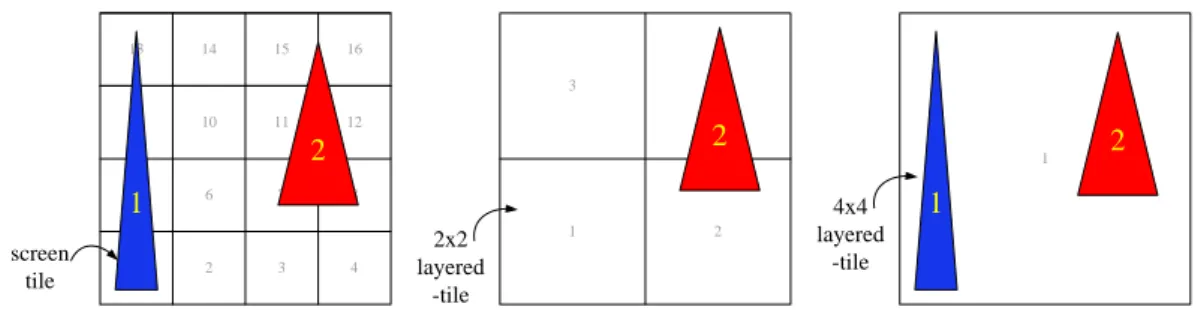
ARM has proposed a hierarchical listing mechanism [5] to store primitive lists in tile-based rendering. As Figure 2-7, the left one is called bottom layer which is the same as typical flat tiling mechanism, each entry represents a screen tile. The other two layers are called grouped layers; each entry is grouping by multiple screen tiles to form an NxN layered-tile. For example, a 2x2 layered-tile consists of 4 tiles in bottom
1 1 2 3 5 6 7 9 10 11 4 8 12 13 14 15 16 1 2 3 4 tile 2x2 layered -tile 4x4 layered -tile
layer, 2 tiles in height and 2 tiles in width. A 4x4 layered-tile consists of 16 tiles in bottom layer, 4 tiles in height and 4 tiles in width and so on. These extra layered-tiles have their own primitive lists to store primitive address in scene buffer. And every layered-tile in upper layer can be use to represent the tiles it represents in bottom layer, which means we can use less primitive list storage if we can store primitives in these layers. For instance, if a primitive’s bounding box covers tile 1, 2, 5 and 6. We can record this primitive with only one record in primitive list of layered-tile 1 in 2x2 layer instead of 4 records in tile 1, 2, 5, and 6’s primitive lists. Although this mechanism can reduce lot of list storage size, it requires to going through all layers to get all corresponding primitive information in rendering a screen tile instead of typical flat primitive list which traverses its own primitive list only.
Figure 2-8 Flow-chart of ARM proposed layer selection algorithm
As Figure 2-8 shows, this patent proposed an algorithm that test primitives layer
by layer, to choose which layer in hierarchy should be used to store this primitive during tile binning process. This algorithm starts with one layer below top (the highest) layer, if number of (layered-)tiles covered by input primitive’s bounding box is below a threshold (e.g., 4) then step down one layer, repeat this process until number of (layered-)tiles covered by bounding box which no longer below a threshold or it reaches a bottom layer. Furthermore, if it is below the threshold then we store in one layer above current layer or if it is in the bottom layer then we store this primitive immediately. Finally it checks if this primitive is a misalignment one or not. If it’s, step down one layer and store primitive into current layer; if it’s not, store to current layer.
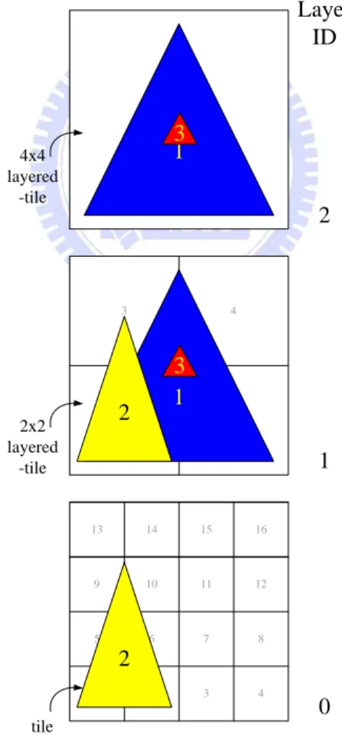
Figure 2-9 Use of ARM’s square hierarchies 1 1 2 3 5 6 7 9 10 11 4 8 12 13 14 15 16 1 2 3 4 tile 2x2 layered -tile 4x4 layered -tile 2 1 1 2 3 3 Layer ID 2 1 0
As Figure 2-9 shows, the testing procedure for triangle No.1 will start from layer 1 which is one layer below top layer. Triangle No.1 covers 4 layered-tiles in layer 1 which excess threshold then we step up one layer to layer 2 and check it is special case or not. Triangle No.1 will be identified as normal case and then store in layer 2. The triangle No.2 will be tested from layer 1, too. And found that it is below threshold which needs to step down one layer to layer 0. Triangle No.2 covers 6 tiles in layer 0 which excess threshold and will be step up one layer and so on. Triangle No.3 is used to demonstrate special case which called misalignment. Triangle No.3 covers 4 layered-tiles in layer 1 and will be step up one layer to layer 2. Then this triangle will be identified as special case because this triangle is lying on the boundary of multiple tiles across different layers which need to step down one layer and store in layer 1.
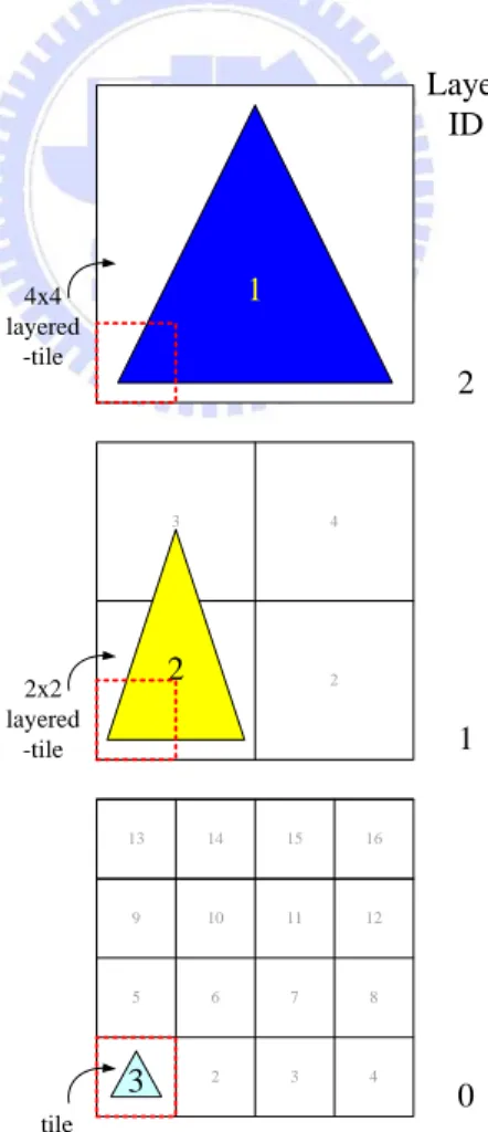
Figure 2-10 Rendering from hierarchical primitive lists 1 1 2 3 5 6 7 9 10 11 4 8 12 13 14 15 16 1 2 3 4 tile 2x2 layered -tile 4x4 layered -tile 1 2 3 Layer ID 2 1 0
After tile binning process, all primitives in current frame are binned into different layers of square hierarchical primitive lists according to the size and position of primitives’ bounding boxes. Rendering a tile from such hierarchical primitive list, it needs to traverse all layers to find out which layered-tile covers current rendering tile and then fetch corresponding primitive list to render. As Figure 2-10 shows, if we need to render tile No.1 of screen, we need the primitive lists of tile No.1 in layer 0, layered-tile No.1 in layer 1 and layered-tile No.1 in layer 2 in order to draw the correct results.
In the patent, it uses only square fashion like 2x2, 4x4, and NxN layered-tile to illustrate their hierarchies. Although this patent claims we can group tiles in any fashion, it doesn’t provide any examples and corresponding layer selection algorithm. This paper will implement the hierarchical list ideas and use different grouping rules to see the effects for the storage size. Also, a new layer selection algorithm which can be easily implemented by hardware will be proposed.
Chapter 3 Design
In this chapter, we will introduce ours layer design according to our observation and a simple algorithm to classify primitives into different layers will proposed. Finally, a layer-based rendering will be introduced which can further reduce external memory traffic in rendering progress.
3.1
Layer design overview
Figure 3-1 Layer design overview
(a) Hierarchical primitive list structure showing all possible hierarchies and shapes
Figure 3-1 shows the overview of our new design layers, the left most part is as same as ARM’s demonstration in their patent. Layer 0 represents the bottom layer which every entry is as same as screen tile, layer 1 represents 2x2 layer, layer 2 represents 4x4 layer and so on. Based on the mechanism proposed by ARM, we introduce unaligned grids to store misalignment primitives and rectangular layers to store primitive of non-square shapes in the middle and the right most of the figure. Details will be discussed in section 3.2 and 3.3. Figure 3-1(b) is the organization of primitive lists in memory. The Prim list presents square hierarchy method’s primitive lists. The UG List represents unaligned grids’ lists. And the HRect (Horizontal Rectangle) List and VRect (Vertical Rectangle) List represent the primitive lists of rectangular layer in high or wide shape. And the X, Y, Z, W indicates the largest layered-tile IDs in upper layers.
3.1.1 Use of Rectangular layers
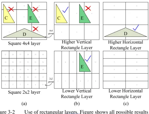
Since high and wide rectangle shapes of primitives are common, we introduce a new layer called rectangular layer to store these kinds of primitives. Except the layer that includes all tiles in screen in single layered-tile, every layer has a corresponding rectangular layer including the bottom layer. As Figure 6(b)(c) show, there are two types of this rectangular layer. First is in high rectangle shape and second in wide rectangle shape. The rules to form these layers are; divide the screen into half based on how many tiles in vertical and horizontal directions of screen to align bottom layer’s tile. The width of high rectangle shape is exactly the same with the corresponding layer’s group width. The height of the wide one is also the same with corresponding layer’s group height.
Figure 3-2 Use of rectangular layers. Figure shows all possible results of primitive-hierarchy fitting and final selections
The rule to classify the primitives into this layer is depending on the difference between tile-based bounding box’s width and height. If the difference between height and width of bounding box reach a threshold (e.g., 2, 4 tiles), then this primitive will be recognized as in rectangular layer. In the Figure 6(c)(c), the primitive C and D will be recognized as in high and wide shape, such that C and D can be stored in rectangular layer with less primitive lists. In this type of layer, we will encounter the misalignment problem. For example, primitive E in Figure 6(b) is a misalignment one. Either 2x2 or 4x4 grouped layers’ rectangular layer, primitive E covers two groups. In this case, we still store primitive E in rectangular layer but step down one layer from where it originally chose as long as it is not the bottom layer.
3.1.2 Use of Unaligned Grids
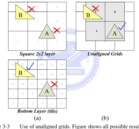
primitives. In this layer, each grouped layers have a corresponding unaligned grid except the layer that includes all tiles in screen in single layered-tile and bottom layer. As Figure 3-3(b) shows, this grid starts from (0 + group-width/2, 0 + group-height/2) with same group size to its corresponding grouped layers. For instance, the misalignment primitive A in Figure 3-3(a), both 2x2 grouped and bottom layers for this primitive requires 4 layered-tiles are recorded. If this unaligned grid is applied, this primitive A can be recorded in this unaligned grid with only one primitive list in Figure 3-3(b).
Figure 3-3 Use of unaligned grids. Figure shows all possible results of primitive-hierarchy fitting and final selections
In Figure 3-3(a), there’s another example primitive B. This primitive is also a misalignment one, but it can not be fit in 2x2 grouped layer’s unaligned grid, because these grids are begin from (0 + group-width/2, 0 + group-height/2) which means there have some tiles this grid cannot be covered. In this case, the primitive B will be stored in square hierarchy and step down one layer as ARM’s patent did. There are two main rules to decide a primitive can be put in this grid or not. First, this primitive must be
misalignment. Second, the primitive’s bounding box need to pass the boundary check which tests this primitive whether it can be covered in this layer or not.
3.1.3 Summary
In this section, we will show the extra overheads in such design. In a hierarchical layer design can reduce storage size requirements, but every primitive in any layered-tile of upper layer will be processed by the tiles it represents. However, some of primitive in the upper layer may cover only half of the area in layered-tile. This would cause extra traffic to fetch these primitives.
Figure 3-4 Redundant access in hierarchical lists
As Figure 3-4, the triangle above will be store in 2x2 layer and the bounding box test result shows this triangle covers two layered-tiles in 2x2 layer, which means tiles 1, 2, 5, 6, 9, 10, 13 and 14 would need to access this triangle when rendering in progress. If we do use typical rendering hardware and policy, we would generate some redundant access in runtime.
To add these extra layers, we will need extra primitive lists to record scene buffer addresses of primitives for these layers. Total number of original primitive list is,
1 2 3 5 6 7 9 10 11 4 8 12 13 14 15 16 1 2 3 4 tile 2x2 layered -tile
To add ARM’s square hierarchies, we would need extra lists below. Assume we have layers from 0 to N,
To add our rectangular layer, we would need extra lists below. Assume we have layers from 0 to N, and layered-tile in layer N can use only one list to includes the whole screen,
To add our unaligned grids, we would need extra lists below. Assume we have layers from 0 to N, and layered-tile in layer N can use only one list to includes the whole screen,
3.2
The Primitive-Hierarchy Fitting Algorithm
To selection of a suitable layer for primitives much faster, we will improve the algorithm proposed by ARM. The primitive-hierarchy fitting algorithm we proposed to select appropriate layer in square hierarchy is in Figure 3-5.
⎡
⎤ ⎡
⎤
(
)
∑
N ScreenWidth LayeredTileWidth × ScreenHeight LayeredTileHeight1 / /
⎡
⎤ ⎡
⎤
(
)
∑
−1 × + × 0 2 / / 2 N eWidth LayeredTil h ScreenWidt eHeight LayeredTil ht ScreenHeig⎡
⎤
(
)
(
⎡
⎤
)
[
]
∑
−1 − × − 1 1 / 1 / N eHeight LayeredTil ht ScreenHeig eWidth LayeredTil h ScreenWidtFigure 3-5 The primitive-hierarchy fitting algorithm for square and aligned
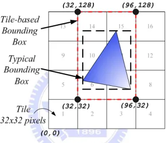
Figure 3-6 Tile-based Bounding Box construction. Inner one is the typical bounding box, and outer one is the tile-based bounding box. The
width of tile-based bounding box is 2 and height is 3.
To understand this algorithm, we need to define layer ID first. The bottom layer is layer 0, 2x2 grouped layer is layer 1, 4x4 grouped layer is layer 2 and so on (as Figure 3-1(a) shows). The boundaries of these layered-tiles are power of 2 and groups together to form upper layers’ layered-tiles. Assume we are using 32x32 pixels as our tile size. When the primitive comes, we first construct its tile-based bounding box as in Figure 3-6. The reason to construct such tile-based bounding box is reducing the complexity of computation circuit. The advantage of such bounding box is that it can easily find out the tile-based length of this bounding box and figure out misalignment or not by searching low-order bits of its coordinate directly. To build such bounding
Step 1. Represent primitive with tile-based bounding box
Step 2.(a) Select the shorter side of the bounding box as reference side
(b) Perform ceil( log2 length-of(Ref-Side) ) to get layer ID
Step 3. Check the input primitive on selected layer is misalignment or not
Yes) Step down one layer and store this primitive
box we will round down minimum X and Y value to nearest multiple of 32, if it is on the boundary then leave it on that boundary. And round up the maximum X and Y value to nearest multiple of 32, if it is on the boundary then shift it to next multiple of 32 in order to detect the correct tile-based length of bounding box. Also, the coordinates of tile-based bounding box are all multiple of 32 which can reduce computation complexity of hardware.
After building up the tile-based bounding box, we will select an appropriate layer to store input primitive in square hierarchies. Since all length and positions of tiles and layered-tiles are power of 2. The relationships between layered-tiles in different layers are power of 2, too. To determine which layer should use to store current primitive we might have multiple choices like shorter side, longer side or average length of tile-based bounding box. Because of the power of 2 characteristic of layered-tile’s length in each side, we can use this side’s tile-based length to perform log2 operation to figure out which layer in hierarchy should we put the primitive in. If
the length of the side is not multiple of two, the result of log2 operation will contain
both integer and non-zero numbers after decimal place. In order to find fittest layered-tile, we will perform a ceiling operation after log2, such that we can round up
to nearest layer which can use exactly one layered-tile to cover this bounding box’s width or height.
Figure 3-7 Effects of different reference side in our algorithm 1 1 2 3 5 6 7 9 10 11 4 8 12 13 14 15 16 1 2 3 4 screen tile 2x2 layered -tile 4x4 layered -tile 1 2 2 2 1
As Figure 3-7 above, if we choose longer side of triangle No.1 as reference side and perform log2 and ceiling operations, we will get layer ID is 2 and store it with a
4x4 layered-tile. Although, we can record this primitive with only one layered-tile, most of the screen tiles covered by this 4x4 layered-tile are not covered by this primitive. And it generates 12 unnecessary accesses in rendering. If we choose shorter side as our reference side, triangle No.1 will be recorded in layer 0 with 4 tiles. And this selection would make the shape of final selection result more suitable for this primitive and reduces unnecessary accesses in rendering. If we take another triangle, said triangle No.2 as example. If we choose longer side, this primitive will be recorded in layer 2 which generates 10 useless accesses in rendering. Otherwise, if we choose shorter side as reference side, this primitive will be recorded in layer 1 with 2 layered-tiles which generates 2 useless accesses in rendering. In our algorithm, we choose shorter side as reference side to discover a balance between useless accesses in rendering and storage size requirements.
Figure 3-8 Building lookup table and circuit for Layer ID generation 100 1111 15 100 … … 100 1010 10 100 1001 9 011 1000 8 011 0111 7 011 0110 6 011 0101 5 010 0100 4 010 0011 3 001 0010 2 000 0001 1 layerID Input (DCBA) Length 100 1111 15 100 … … 100 1010 10 100 1001 9 011 1000 8 011 0111 7 011 0110 6 011 0101 5 010 0100 4 010 0011 3 001 0010 2 000 0001 1 layerID Input (DCBA) Length
Layer ID Generation:
if ( Input > 810 ) LID= 1002 (410) else LIDbit-0 = A + BD + CD’ LIDbit-1 = A + B + CD LIDbit-2 = 0Although the logarithm and ceiling functions will need complex circuit and longer cycle time to finish, our implementation will use a simple way to replace these calculations. Typically, implementation of hierarchical primitive list will use limited layers to ensure hardware’s simplicity. So we can build a lookup table for this logarithm and ceiling operation, and this table can be further reduced via Karnaugh Map. As Figure 3-8 shows, assume we have five layers in our implementation with Layer ID 0 to 4. If length of reference side is larger than 10002 (810) in tiles, then
output the layer ID 1002 (410) directly. The others we can use LSB 4-bit from length of
reference side in tiles as input to generate 3-bit layer ID. Let input bits from bit-0 to bit-4 be A, B, C, and D. The output bit-0 can be expressed by A + BD + CD’, bit-1 A + B + CD and keep bit-2 always zero. Combine the rules above; we can build the Layer Select Logic to get the Layer ID in a simple circuit.
Figure 3-9 Circuit implementation of the primitive-hierarchy fitting algorithm. Note that this circuit is a combinational logic. The algorithm steps
simply indicates flow of signals, but not states
Primitive B B ox Height Primit ve BB ox Width
To detect the misalignment, we can use an intuitive way since the length of both sides of layered-tiles in square hierarchies are in power of 2; such that we can detect misalignment by directly detect the low-order bits of 4 coordinates (maximum and minimum X, Y) of tile-based bounding box. Put these rules and Layer Select Logic together, we can form our circuit of layer fit algorithm.
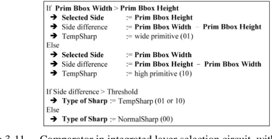
Figure 3-9 shows the circuit implementation of primitive-hierarchy fitting algorithm. The comparator takes the input primitive’s tile-based bounding box’s width and height in number of tiles. Then output shorter side as reference side to the Layer Select Logic. The output of Layer Select Logic will be the layer ID. And the four multiplexors will check the maximum and minimum X, Y positions’ values to see whether the primitive in selected layer is misalignment or not. Since typical tile size is 32x32 pixels, the coordinates including tiles and groups must be a multiple of 32. We can determine the input primitive is misalignment or not by checking the low-order bits of its tile-based bounding box’s coordinates. If it is a misalignment then outputs layer ID -1 (step down one layer). If it’s not, outputs the selected layer ID from Layer Select Logic.
As the layer design described in section 3.1, we design two new layers called unaligned grids and rectangular layers. Both these designs have a same characteristic with square hierarchies. For unaligned grids, the height and width of a layered-tile is exactly the same with corresponding layered-tile in square hierarchies. For rectangular layers, the width of vertical rectangle and the height of horizontal rectangle are exactly the same with corresponding layered-tile in square hierarchies. Due to this characteristic, the Layer Select Logic used in Figure 3-9 can be applied in choose appropriate layer to store primitive in unaligned grids and rectangular layers.
Figure 3-10 Circuit implementation of the primitive-hierarchy fitting algorithm, with fittings to rectangle and unaligned grid variations included
Integrate unaligned grids and rectangular layers with this algorithm. We need to give priorities in order to choose which type of layer is more appropriate to use. In our implementation, the rectangular layer has highest priority and then unaligned grid in the next place, finally square hierarchy is the lowest one. Also, we need to add an output to indicate what type of layer to use alone with layer ID.
Figure 3-11 Comparator in integrated layer selection circuit, with behavior description only Type of S h a rp P rim iti v e BBo x Heig ht P ri m it ve BB ox Wi dth
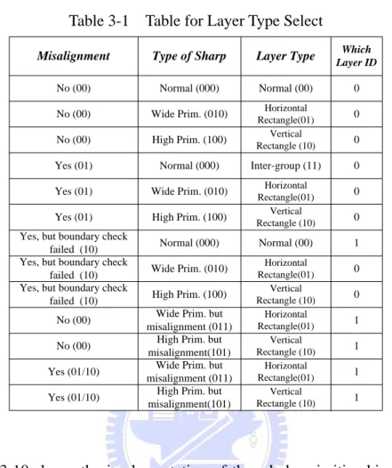
Table 3-1 Table for Layer Type Select Type of Sharp
Misalignment Layer Type
No (00) No (00) Yes (01) Yes (01) Normal (000) Wide Prim. (010) Normal (00) Horizontal Rectangle(01)
High Prim. (100) Vertical
Rectangle (10) No (00) Yes (01) Normal (000) Wide Prim. (010) High Prim. (100) Inter-group (11)
Yes, but boundary check failed (10) Yes, but boundary check
failed (10) Yes, but boundary check
failed (10) Normal (000) Wide Prim. (010) High Prim. (100) Normal (00) Which Layer ID 0 0 0 0 0 0 1 0 0 Wide Prim. but
misalignment (011) High Prim. but misalignment(101) No (00) Yes (01/10) Yes (01/10) No (00) 1 1 1 1 Wide Prim. but
misalignment (011) High Prim. but misalignment(101) Horizontal Rectangle(01) Vertical Rectangle (10) Horizontal Rectangle(01) Horizontal Rectangle(01) Horizontal Rectangle(01) Vertical Rectangle (10) Vertical Rectangle (10) Vertical Rectangle (10)
Figure 3-10 shows the implementation of the whole primitive-hierarchy fitting algorithm. The priorities of these different types of hierarchies are encoded in the lookup table as Table 3-1 shows. As Figure 3-11 shows, once the comparator determines this input bounding box whether it is a high or wide rectangle, this primitive will be stored in rectangular layer corresponding to selected layer ID. But if misalignment is found in Misalignment Check, then it will output this information together to Layer Type Select in order to make the correct layer decision. The unaligned grid will be used if this bounding box is misalignment and passed the Boundary Check. Finally, if this bounding box cannot be classified as either rectangular or unaligned grid, then this primitive will be stored in square hierarchies.
3.3
Primitive list design
As section 2.2.2, the typical data structure of primitive list would have serious storage waste or internal fragmentation. In this section, we will propose a primitive list design to reduce these problems.
Figure 3-12 Primitive list design
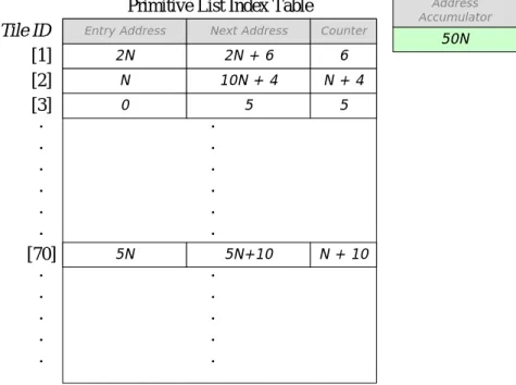
As Figure 3-12, we combine multiple scene buffer addresses as one block with a next address pointer in last entry of it. The block size N is power of 2 which can be 4, 8, 16 and 32 or higher. This List Buffer is initially unassigned, once a primitive list requires a record it will check the Primitive List Index Table first.
Figure 3-13 Primitive list management in GPU
As Figure 3-13 shows, each tile has a corresponding entry in the Primitive List
Index Table which records the starting address of its primitive list in List Buffer, also
the next available address for recording scene buffer address and a Counter to record how many primitives have been record into this primitive list. This Primitive List
Index Table is initially empty, once we require a scene buffer address to be recorded
in a specific tile’s primitive list, it will check the Entry Address of corresponding entry in Primitive List Index Table to see it is NULL or not. If it is a NULL means this entry is the first time to be used, then it will check List Buffer’s address accumulator to see the address of next available block in List Buffer and then assign this address into this Entry Address, also the address accumulator would plus N into it. If it is not NULL, it will check if Counter field reaches multiple of N-1, if it is, it means that this block is full, then request for a new block in List Buffer and assign this new block’s address into current block’s Next address field. Others, simply write the scene buffer address into the address indicate by Next Address field and update this Next Address and Counter fields after writing the address into it.
Primitive List Index Table
[1] 2N 2N + 6 N 10N + 4 0 5 [2] [3] 5N 5N+10 [70]
Tile ID Entry Address Next Address Counter
6 N + 4 5 N + 10 50N Address Accumulator
Figure 3-14 Square Hierarchical Primitive list management in GPU
If we are using a hierarchical primitive list structure like square hierarchies, we can simply add a Layer Offset Table to indicate base address of each layer. As Figure 3-14 shows, the Primitive List Index Table remains the same, all tiles and layered-tiles have a corresponding entry in it but into several different segments. First segments for bottom layer’s tiles and second segments for layer 1’s layered-tiles and so on. Once we need to find an entry in Primitive List Index Table, it needs to add (layered-)tile ID and base address in Layer Offset Table together and then this result can be used to index corresponding entry in Primitive List Index Table.
Primitive List Index Table
[1] 2N 2N + 6 N 10N + 4 0 5 [2] [3] 5N 5N+10 [70]
Tile ID Entry Address Next Address
Layer Offset Table
0 80 100 Offset Layer ID [0] [1] [2] [3] Counter 6 N + 4 5 N + 10 50N Address Accumulator
Figure 3-15 Ours Hierarchical Primitive list management in GPU
In our design, we have three different types of hierarchies. To index such multiple hierarchies in same Primitive List Index Table, we need to modify the structure of Layer Offset Table. As Figure 3-15 shows, the Layer Offset Table need to be extended to two dimensional, one for layer ID and one for which type of hierarchies. In our design, we have three different hierarchies, but the rectangular layers have two variants so we need two entries for rectangular layers. Such that, we will have a two dimensional Layer Offset Table with NumberOfLayers * 4 entries.
Since we have a generalize storage for records in primitive list, we only need to add entries in Primitive List Index Table without enlarge size of List buffer.
Primitive List Index Table
[1] 2*N 2*N + 6 N 10*N + 4 0 5 [2] [3] NULL NULL [81] [82] NULL NULL
Tile ID Entry Address Next Address Counter 6 N + 4 5 0 0 50N Address Accumulator
Layer Offset Table
0 80 100 Offset Layer ID [0] [1] [2] [3] 120 200 220 Offset Layer Type 240 320 340 Offset 360 440 460 Offset
Chapter 4 Evaluation Results & Discussion
In this section we will demonstrate our simulation results. We first describe our evaluation environment and the characteristics of the input frame data (in section 4.1 and 4.2). Then, we show and analyze the simulation results of memory requirement and memory traffic overhead in rendering of our method. Finally, the discussion will be shown. 4.1
Evaluation Environment
Primitive1: {x1,y1,z1},{x2,y2,z2},{x3,y3,z3},Bbox Primitive2: {x1,y1,z1},{x2,y2,z2},{x3,y3,z3},Bbox ………Tile-based Rendering
Software Behavior
Simulator
Figure 4-1 Simulation flow and ATTILA architectureWe choose Doom3[7] and Quake4[8] as our benchmarks with resolution 320x240, 640x480, 1280x1024 and 1600x1200, 20 frames from frame 30 to 600 with 30 frames as interval. Figure 4-1 shows the architecture of GPU simulator ATTILA[6] and in which stage we dump the transformed primitives from. Then use this dumped tracefile as input to our tile-based rendering software behavior simulator. Our simulator reads these transformed vertices data from tracefile and evaluates storage size and memory access traffic in rendering of primitive lists. The results below are average of the five frames and tile size is 32x32 pixels. The algorithm in section 3.2 is also applied.
4.2
Number of Layers versus Screen Resolution in Square
Hierarchies
First we will look at the relationships between number of layers and screen resolutions. The first part of this section will show the storage reduction rate from various resolutions and number of layers. And second part of this section will show the access traffic in rendering.
Doom3 320x240, Number of Layers vs. Records Reduction
0.00 5.00 10.00 15.00 20.00 25.00 30.00 35.00 40.00 45.00 50.00
2 Layers 3 Layers 4 Layers 5 Layers 6 Layers 7 Layers
St or ag e R edu ct io n (% )
Proposed Alg ARM
aligned hierarchies versus flat list version
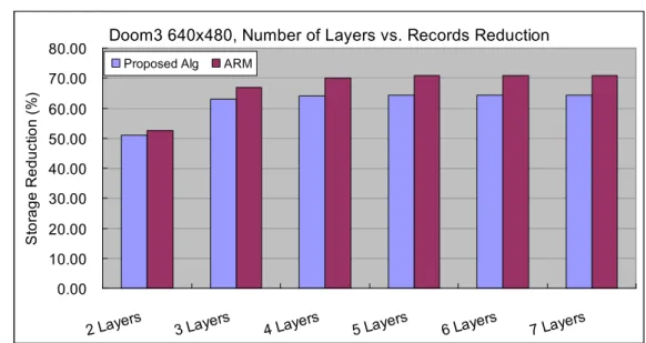
Doom3 640x480, Number of Layers vs. Records Reduction
0.00 10.00 20.00 30.00 40.00 50.00 60.00 70.00 80.00
2 Layers 3 Layers 4 Layers 5 Layers 6 Layers 7 Layers
St or ag e R edu ct io n (% )
Proposed Alg ARM
Figure 4-3 Doom3 640x480 storage reduction percentages by using square and aligned hierarchies versus flat list version
Doom3 1280x1024, Number of Layers vs. Records Reduction
0.00 10.00 20.00 30.00 40.00 50.00 60.00 70.00 80.00 90.00 100.00
2 Layers 3 Layers 4 Layers 5 Layers 6 Layers 7 Layers
St or ag e R edu ct io n (% )
Proposed Alg ARM
Figure 4-4 Doom3 1280x1024 storage reduction percentages by using square and aligned hierarchies versus flat list version
Doom3 1600x1200, Number of Layers vs. Records Reduction 0.00 10.00 20.00 30.00 40.00 50.00 60.00 70.00 80.00 90.00 100.00
2 Layers 3 Layers 4 Layers 5 Layers 6 Layers 7 Layers
St or ag e R edu ct io n (% )
Proposed Alg ARM
Figure 4-5 Doom3 1600x1200 storage reduction percentages by using square and aligned hierarchies versus flat list version
Quake4 320x240, Number of Layers vs. Records Reduction
0.00 10.00 20.00 30.00 40.00 50.00 60.00
2 Layers 3 Layers 4 Layers 5 Layers 6 Layers 7 Layers
St or ag e R edu ct io n (% )
Proposed Alg ARM
Figure 4-6 Quake4 320x240 storage reduction percentages by using square and aligned hierarchies versus flat list version
Quake4 640x480, Number of Layers vs. Records Reduction 0.00 10.00 20.00 30.00 40.00 50.00 60.00 70.00 80.00
2 Layers 3 Layers 4 Layers 5 Layers 6 Layers 7 Layers
S tor ag e R educ tion (% )
Proposed Alg ARM
Figure 4-7 Quake4 640x480 storage reduction percentages by using square and aligned hierarchies versus flat list version
Quake4 1280x1024, Number of Layers vs. Records Reduction
0.00 10.00 20.00 30.00 40.00 50.00 60.00 70.00 80.00 90.00 100.00
2 Layers 3 Layers 4 Layers 5 Layers 6 Layers 7 Layers
S to rag e R educt ion (% )
Proposed Alg ARM
Figure 4-8 Quake4 1280x1024 storage reduction percentages by using square and aligned hierarchies versus flat list version
Quake4 1600x1200, Number of Layers vs. Records Reduction 0.00 10.00 20.00 30.00 40.00 50.00 60.00 70.00 80.00 90.00 100.00
2 Layers 3 Layers 4 Layers 5 Layers 6 Layers 7 Layers
S tor age R educt io n (% )
Proposed Alg ARM
Figure 4-9 Quake4 1600x1200 storage reduction percentages by using square and aligned hierarchies versus flat list version
As Figure 4-2 to 4-9 shows, the y-axis is the percentage of storage reduction compare to typical flat tile-listing. And x-axis is different number of layers; the different number of layer setting from 2 layers that’s typical tiling with 2x2 grouped layer, 3 layers is typical tiling with 2x2 and 4x4 grouped layers, and so on. Different color of bars are using square hierarchies with ARM’s algorithm or ours primitive-hierarchy fitting algorithm. In lower resolution 320x240 in both benchmarks, three layers is enough for these two resolutions, since both of them use more layers which cannot gain more storage reductions. For higher resolutions, four layers would be a good choice, since the difference of size reduction between four and five layers is not significantly obtained. As the observation in section 2.3, there’s less primitives that overlap on exact one tile as the screen resolution gets higher. The result in Figure 4-2 to 4-9 shows the same characteristic, as the resolution gets higher then this square hierarchies can save more storage.
Doom3 320x240, Number of Layers vs. Redundant Read 0 10000 20000 30000 40000 50000 60000 70000 80000
2 Layers 3 Layers 4 Layers 5 Layers 6 Layers 7 Layers
Re
co
rd
s
Proposed Alg ARM
Figure 4-10 Doom3 320x240 redundant reads by using square and aligned hierarchies
Doom3 640x480, Number of Layers vs. Redundant Read
0 50000 100000 150000 200000 250000 300000 350000
2 Layers 3 Layers 4 Layers 5 Layers 6 Layers 7 Layers
Re
co
rd
s
Proposed Alg ARM
Figure 4-11 Doom3 640x480 redundant reads by using square and aligned hierarchies
Doom3 1280x1024, Number of Layers vs. Redundant Read 0 200000 400000 600000 800000 1000000 1200000 1400000 1600000 1800000
2 Layers 3 Layers 4 Layers 5 Layers 6 Layers 7 Layers
Re
co
rd
s
Proposed Alg ARM
Figure 4-12 Doom3 1280x1024 redundant reads by using square and aligned hierarchies
Doom3 1600x1200, Number of Layers vs. Redundant Read
0 500000 1000000 1500000 2000000 2500000 3000000
2 Layers 3 Layers 4 Layers 5 Layers 6 Layers 7 Layers
Re
co
rd
s
Proposed Alg ARM
Figure 4-13 Doom3 1600x1200 redundant reads by using square and aligned hierarchies
Quake4 320x240, Number of Layers vs. Redundant Read 0 10000 20000 30000 40000 50000 60000 70000
2 Layers 3 Layers 4 Layers 5 Layers 6 Layers 7 Layers
Re
co
rd
s
Proposed Alg ARM
Figure 4-14 Quake4 320x240 redundant reads by using square and aligned hierarchies
Quake4 640x480, Number of Layers vs. Redundant Read
0 50000 100000 150000 200000 250000 300000
2 Layers 3 Layers 4 Layers 5 Layers 6 Layers 7 Layers
Re
co
rd
s
Proposed Alg ARM
Figure 4-15 Quake4 640x480 redundant reads by using square and aligned hierarchies
Quake4 1280x1024, Number of Layers vs. Redundant Read 0 200000 400000 600000 800000 1000000 1200000 1400000 1600000
2 Layers 3 Layers 4 Layers 5 Layers 6 Layers 7 Layers
R
ecor
ds
Proposed Alg ARM
Figure 4-16 Quake4 1280x1024 redundant reads by using square and aligned hierarchies
Quake4 1600x1200, Number of Layers vs. Redundant Read
0 500000 1000000 1500000 2000000 2500000
2 Layers 3 Layers 4 Layers 5 Layers 6 Layers 7 Layers
Re
co
rd
s
Proposed Alg ARM
Figure 4-17 Quake4 1600x1200 redundant reads by using square and aligned hierarchies
As Figure 4-10 to 4-17 shows, the y-axis is the total number of redundant records read during rendering. And x-axis is different number of layers with different color of bars for ours and ARM’s algorithm. From the figure above, we can see that our method would lead to about 5% more storage usages compare to ARM’s method. The results from Figure 4-10 to 4-17 show the advantages of our primitive-hierarchy
fitting algorithm. Our algorithm can choose better layer than ARM did. Such that, the redundant reads in our design are significantly lower than ARM in any benchmarks and resolutions.
4.3
Storage Reduction of Proposed Design
The effect of applying unaligned grids and rectangular layers will be shown in the following. The baseline is using square hierarchies only. The number of layers will be fixed by the results we observed above. For lower resolution 320x240, we will use three layers in the following experiments and for the higher resolutions, we will use four layers.
Doom3, Storage Reduction of Proposed Design
0.00 10.00 20.00 30.00 40.00 50.00 60.00 70.00 80.00 90.00 100.00 320x240 640x480 1280x1024 1600x1200 Resolutions P rim iti ve S tor age S iz e R educ tio n (% )
ARM Proposd Alg.
Proposed UG Proposed RL
Proposed Full Capa.
Figure 4-18 Doom3 storage reductions by proposed design versus square and aligned version
Quake4, Storage Reduction of Proposed Design 0.00 10.00 20.00 30.00 40.00 50.00 60.00 70.00 80.00 90.00 100.00 320x240 640x480 1280x1024 1600x1200 Resolutions P rim iti ve S tor age S iz e R educ tio n (% )
ARM Proposd Alg.
Proposed UG Proposed RL
Proposed Full Capa.
Figure 4-19 Quake4 storage reductions by proposed design versus square and aligned version
Figure 4-18 and 4-19 shows the percentage of storage reduction compare to use square hierarchies only with both ARM’s and ours algorithm, when adding grouping methods we described it in section 3.1. The unaligned grids can reduce tile list size about 1% to 10% since the misalignment primitive various from 2% to 20% in various test cases with our algorithm, but still a little bit more than ARM’s algorithm with square hierarchies only. For the rectangular layer, we set different thresholds for different resolutions according to how many tiles need to cover the height of screen. For instance, in 320x240 we need 8 tiles to cover the height of 240 pixels, since rectangular layers split screen into two parts, so we require the difference of primitive’s height and width need to be larger than 2 tiles in order to use these layers more efficient. For the same reason, we choose 4 for 640x480, 8 for 1280x1024 and 10 for 1600x1200. Although the high and wide rectangle of primitives is about 35% in our observation in section 3.1, the result here is a bit different. One reason is the threshold; another reason is some of primitives are lying in the middle of the screen and it requires two or more groups to record. Again, when applying our rectangular layer and our algorithm, we still need a little big larger storage than ARM did.
When apply both unaligned grids and rectangular layers together, we can achieve 5% of storage reduction compare with our algorithm and square hierarchies only. The storage reduced by both type of layers can not be added together directly. It caused by the primitive-hierarchy fitting algorithm sets higher priority for rectangular layer and part of misalignment primitive will be covered into this layer and no longer seen as a misalignment. When apply both layers together our storage size requirement will be more like ARM did.
Doom3, Redundant Read of Proposed Design
0.00 200000.00 400000.00 600000.00 800000.00 1000000.00 1200000.00 1400000.00 320x240 640x480 1280x1024 1600x1200 Resolutions Re co rd s
ARM Proposed Alg.
Proposed UG Proposed RL
Proposed Full Capa.
Quake4, Redundant Read of Proposed Design 0.00 200000.00 400000.00 600000.00 800000.00 1000000.00 1200000.00 1400000.00 1600000.00 1800000.00 320x240 640x480 1280x1024 1600x1200 Resolutions Re co rd s
ARM Proposed Alg.
Proposed UG Proposed RL
Proposed Full Capa.
Figure 4-21 Quake4 redundant reads by proposed design
Figure 4-20 and 4-21 above shows the redundant reads by proposed layer designs. In both figure, we can see that when adding our layer designs together, the redundant reads are significantly higher than ARM did. The reason for this result is that many misalignment primitives are now can be recorded in higher layer which would lead to more unnecessary traffics. And the rectangular layer, some of the primitives are lying across multiple horizontal rectangle or vertical rectangle layered-tiles. Such that, combining both leads to this result.
4.4
Storage Requirement of Proposed List Buffer
In this section, we will evaluate the storage size requirement between various size of block used in our List Buffer with square hierarchies only.
Figure 4-22 Doom3 List buffer size requirements
Figure 4-23 Quake4 List buffer size requirements
0 200000 400000 600000 800000 1000000 1200000 1400000 1600000 1800000 1600 x120 0_2 1600 x120 0_8 1600 x120 0_32 1600 x120 0_12 8 1600 x120 0_51 2 1280 x102 4_2 1280 x102 4_8 1280 x102 4_32 1280 x102 4_12 8 1280 x102 4_51 2 640x 480_ 2 640x 480_ 8 640x 480_ 32 640x 480_ 128 640x 480_ 512 320x 240_ 2 320x 240_ 8 320x 240_ 32 320x 240_ 128 320x 240_ 512 ScnBufAddr NextAddrPtr 0 200000 400000 600000 800000 1000000 1200000 1400000 1600000 1600 x120 0_2 1600 x120 0_8 1600 x120 0_32 1600 x120 0_12 8 1600 x120 0_51 2 1280 x102 4_2 1280 x102 4_8 1280 x102 4_32 1280 x102 4_12 8 1280 x102 4_51 2 640x 480_ 2 640x 480_ 8 640x 480_ 32 640x 480_ 128 640x 480_ 512 320x 240_ 2 320x 240_ 8 320x 240_ 32 320x 240_ 128 320x 240_ 512 ScnBufAddr NextAddrPtr
As Figure 4-22 and 4-23 shows, the y-axis is the total number of records need by List Buffer. And the x-axis is various test cases and sizes of blocks in List Buffer. The block sizes we choose are 2, 4, 8, 16, 32, 64, 128, 256, 512 and 1024. And both results show that when use 8 records in a block can have a balance between List Buffer storage requirement and access time. Which means 7 records for scene buffer pointer and 1 for next block address for a block in List Buffer will be the best choice.
4.5
Discussion
The results in section 4.2 show we can reduce storage requirements by using hierarchical primitive lists. Although misalignment primitive is not major problem in this square hierarchy, the size reduction is still not ignorable. Especially when resolution and number of layer get higher, there will be thousands of primitives are misalignment. The reason we ignore these primitives that can not cover by unaligned grids is that this kind of primitive only holds 8% in average of all misalignment primitives, so we ignore this amount of primitives. The purpose of choosing thresholds in rectangular layer is to use these layers efficiently. If the threshold is too low, the primitives would easily fall into this layer and cover only a few of tiles in rectangular layer’s group which cause extra traffics. So the trade off between traffic and storage reduction by rectangular layer need to be considered carefully.
Although, the result of our primitive-hierarchy fitting algorithm can have significantly less redundant traffic when using square hierarchies only, when applying all layers design seems not. But the generalize the primitive list storage List Buffer, we can add any different shapes of layered-tiles we want. For such hierarchical
primitive lists structure design, we need to trade off between storage size, data traffic and circuit complexity when implement into hardware to get best performance and cost ratio.
Chapter 5 Conclusion and Future Work
5.1
Conclusion
In this paper, we proposed two different grouping methods and a primitive-hierarchy fitting algorithm to enhance the hierarchical mechanism. When we use unaligned grids and rectangular layers together, it can further reduce the primitive storage by 5% compare to use ARM’s square hierarchies only. Also, a new primitive-hierarchy fitting algorithm is proposed which only requires simple circuit to classify primitives into different types of layers. Considering that embedded 3D application become popular and complex, then the corresponding hardware must be developed. We believe tile-based rendering is a suitable technique for such devices. Although it requires external memory to store its primitives’ information, the method we proposed can reduce size to satisfy such devices’ environments.
5.2
Future Work
Primitive Lists Tile Binning Scene buffer Primitive Data 1 Primitive Data 2 Primitive Data N 0xCF110000 0xCF110100 0xCFFFFFFF Frame buffer Tra n sf ormedTriangles CommonShared
Storage Area
Local Buffer Tile Renderer
Local Buffer Tile Renderer
Local Buffer Tile Renderer
Local Buffer Tile Renderer
Figure 5-1 Parallel Tile Renderer Architecture
As Figure 5-1 shows, after tile binning process, the primitives have been classified into hierarchical primitive lists. In pixel processing stages, assuming we will have multiple tile renderers and each of them responsible for drawing a tile in screen. All of these renderers will fetch required primitive lists and primitive data from Shared Common Storage Area, it might an indexable buffer or cache.
There’s an important characteristic of hierarchical primitive lists structure. Once a primitive is identified to store on the layered-tile of upper layer in hierarchy. This primitive will be rendered by the tiles covered by this layered-tile. And the hierarchical primitive lists gather these primitive with sharing properties to upper layers. If we render primitives in upper layer first within a specific region, we can exploit very useful data locality for these primitive data and records in primitive list.
Figure 5-2 Rendering sequence for Parallel Tile Renderers
To render from such hierarchical primitive lists structure, we can use a special render sequence called Recursive-Z [10] to control tile rendering sequence. As Figure 5-2 shows, the tile rendering sequence of screen will be like the alphabet ‘Z’. And each time this recursive process traverse through 4 layered-tiles in upper and lower layers. For example, the first four tiles to be rendered are 1, 2, 7 and 8. Then, this process will step up a layer to Layer 1 and choose 2x2 layered-tile No. 2. And this time, the tiles covered by 2x2 layered-tile No.2 will be rendered, that is tile 3, 4, 9 and 10. Once 2x2 layered-tiles 1, 2, 4, and 5 have been traversed. This process will step up to Layer 2 and choose next 4x4 layered-tile to traverse. The advantage of this process is that no matter how many tile renderers we have, this rendering sequence can keep the primitives in upper layer can be shared by current rendering tiles.
The preliminary result, we set primitive list and primitive data with separate caches. And cache for primitive list is 4-way set-associative and each way with 512-entry, replacement policy depends on maximum reusable times it have. For example, a primitive in a 2x2 layered-tile have maximum reusable times for four. Once it is referenced, then this reusable times will be decreased by 1. If there’s a conflict in cache, it would check whether the new reusable time larger then it was. If it is, replace it. The cache for primitive data is 2-way set-associative and each way with