非擬真卡通動作效果之合成

全文

(1)!. ୮ Ҥ ҫ ೮ δ Ꮱ! !. !. !. !. !. ၅૩࣫Ꮠ‫!ء‬ ᅺ!γ!ፕ!Ў!. 非擬真卡通動作效果之合成 The Synthesis of Non-Photorealistic Motion Effects for Cartoon. 研究生：賴映華指導教授：施仁忠. 教授. ύ!๮!҇!୯!!ΐ!˺!Ѥ!!ԃ!Ϥ!Д!.

(2) !. 非擬真卡通動作效果之合成. 指導教授: 施仁忠教授. 研究生: 賴映華. 國立交通大學資訊科學系. 摘. 要. 在卡通動畫中，動畫師會利用一些不同風格的動作表現手法，來呈現物體的快速移動，而我們稱之為非擬真的動作效果。這些效果不僅是為了表現物體的運動方向，也為了能更烘托出畫面的氣氛，但往往在動畫製作的流程中，動畫師需花費不少額外的時間來完成這些效果。基於此，我們提出了一個系統能更方便且自動化的產生這些效果。此外，為了能更有系統的表現出各式各樣的動作效果，我們將其分類整理，更進一步分析其相關性及差異性，並建置一個適當的流程，讓使用者只需透過參數的設置，便能完成各種效果的繪製。. I.

(3) ). The Synthesis of Non-Photorealistic Motion Effects for Cartoon. Student: Ying-Hua Lai. Advisor: Dr. Zen-Chung Shih. Institute of Computer and Information Science National Chiao-Tung University. ABSTRACT. In cartoon videos, animators use stylistic motion impressions to present fast moving called non-photorealistic motion effects. These motion effects not only represent the direction of motion but also set off the atmosphere by contrast. But, for drawing these effects animators need to spend extra time. According to these, we propose a system to generate these effects automatically. In order to systematically display various effects, we classify them and analyze their linkage and difference. Furthermore, we establish a proper procedure to accomplish painting and animators can create different motion expressions through parametric control.. II.

(4) Acknowledgements. First of all, I would like to express my gratitude to my advisor, Prof. Zen-Chung Shih for his guidance and patience. Also, I appreciate all the members in Computer Graphics and Virtual Reality Laboratory for their comments and help in these days.. I dedicate the achievement of this work to my family and friends, and thanks for their support and encouragement. Special thanks go to my boy friend. Without his support and company, I couldn’t fully focus on my study.. III.

(5) Contents. ABSTRACT (IN CHINESE)....................................................................................... I ABSTRACT (IN ENGLISH) .....................................................................................II ACKNOWLEDGEMENTS ..................................................................................... III CONTENTS............................................................................................................... IV LIST OF TABLES..................................................................................................... VI LIST OF FIGURES .................................................................................................VII CHAPTER 1. INTRODUCTION .............................................................................1. 1.1 Motivation............................................................................................................1 1.2 Overview..............................................................................................................2 CHAPTER 2. RELATED WORKS..........................................................................4. CHAPTER 3. INVESTIGATION OF ANIMATION .............................................6. 3.1 Media of Cartoon Painting...................................................................................6 3.2 Classification of Motion Effects ..........................................................................7 CHAPTER 4 FEATURE EXTRACTION ...............................................................13 4.1 Motion Estimation .............................................................................................13 4.2 Rear Edges and Front Edges ..............................................................................17 CHAPTER 5 GENERATION OF MOTION EFFECTS .......................................20 5.1 Stroke Generation ..............................................................................................20 5.2 Motion Effects: Lines ........................................................................................22 5.2.1 Parallel Straight Lines ................................................................................22 5.2.2 Tracking Curves ..........................................................................................24 5.2.3 Radiative Rays ............................................................................................26 5.3 Motion Effects: After-image ..............................................................................29 5.3.1 Replication of Contours ..............................................................................29 IV.

(6) 5.3.2 Replication of Characters ...........................................................................30 5.4 Motion Effects: Deformation .............................................................................31 5.4.1 Jagged Contours .........................................................................................31 5.4.2 Style Change of Contours ...........................................................................35 CHAPTER 6 IMPLEMENTATION AND RESULTS ............................................36 CHAPTER 7 CONCLUSIONS.................................................................................52 REFERENCE.............................................................................................................54. V.

(7) List of Tables Table 3.1 Classification of Non-photorealistic Motion Effects .....................................8 Table 6.1 The result of motion estimation for Figure6.1 .............................................37 Table 6.2 The result of motion estimation for Figure6.2 .............................................37. VI.

(8) List of Figures Figure 1.1 Example of Non-Photorealistic motion effects ............................................1 Figure 1.2 Flow chart of the system...............................................................................2 Figure 3.1 “The Little Worm” (a) The path for worm (b) The style that is applied (c) A cartoon character with style ...................................................................................7 Figure 3.2 Parallel straight lines (a) Sparser and shorter lines. (b) Denser and longer lines ........................................................................................................................8 Figure 3.3 An example of Tracking curves....................................................................9 Figure 3.4 Radiative rays (Magister Negi Magi) ...........................................................9 Figure 3.5 Replication of contours (a) Full rear edge (b) Gradually decreased rear edge (c) Full contours ..........................................................................................10 Figure 3.6 Replication of character..............................................................................10 Figure 3.7 Jagged contours .......................................................................................... 11 Figure 3.8 Style change of contours ............................................................................ 11 Figure 3.9 Squashed objects (Keroro Kunso) ..............................................................12 Figure 4.1 Motion direction .........................................................................................14 Figure 4.2 Linear Perspective ......................................................................................16 Figure 4.3 Detection of Rear Edges.............................................................................18 Figure 4.4 An Example of Rear Edges: (a) θ = 90° (b) θ = 135°..................................18 Figure 5.1 Stroke generation of straight line painting .................................................21 Figure 5.2 Stroke generation of curve painting ...........................................................21 Figure 5.3 Curve painting (a) Color: black (b) Color: from black to white ................22 VII.

(9) Figure 5.4 The generation of starting points (a) Random (b) Regular random ...........23 Figure 5.5 Cardinal Spline for moving path ................................................................25 Figure 5.6 Paths generation of tracking curves............................................................26 Figure 5.7 Generation of radiative rays: (a) lengths of rays (b) directions and the basic positions ...............................................................................................................28 Figure 5.8 Ranges of shifting distances for replications..............................................30 Figure 5.9 Generation of jagged contours: (a) Regular intervals (b) Determination of intervals and shifting distances with considering the movements (c)Disconnected jags. ......................................................................................................................32 Figure 5.10 The generation of style change of contours..............................................35 Figure 6.1 The first example for motion estimation (School Rumble)........................36 Figure 6.2 The second example for motion estimation (Hime). ..................................37 Figure 6.3 Rear edges (One Piece) (a) Input data (b) Results .....................................38 Figure 6.4 Straight lines applied the random position generator (One Piece) .............39 Figure 6.5 Straight lines applied the position generator with considering movement (One Piece)...........................................................................................................40 Figure 6.6 Curve tracking applied the position generator with considering movement (One Piece)...........................................................................................................41 Figure 6.7 Results of radiative rays (School Rumble).................................................42 Figure 6.8 Rear edges (Keroro Kunso) (a) Input data (b) Results ...............................43 Figure 6.9 Replication of rear edges without decreasing (Keroro Kunso) ..................44 Figure 6.10 Replication of rear edges with decreasing (Keroro Kunso) .....................45 Figure 6.11 Replication of images (Keroro Kunso).....................................................46 Figure 6.12 Jagging contours with the regular interval (Honey and Clover) ..............47 Figure 6.13 Jagging contours applied the interval and length with considering movements (Honey and Clover) ..........................................................................48 VIII.

(10) Figure 6.14 Disconnected jags (Honey and Clover)....................................................49 Figure 6.15 Style change of contours (Magister Negi Magi) ......................................50 Figure 6.16 Result which combines two styles of motion effects (One Piece) ...........51. IX.

(11) Chapter 1 Introduction. 1.1 Motivation Due to more and more stories of caricatures are adapted for animations, many painting skills of comics are applied to animations, such as motion or emotion effects. Many researches [10] show that these kinds of motion effects painted by simple strokes are verity and enough to produce mental image corresponding to real world. For example, in Figure1.1 [2], the speed-lines show the character how to shake its hands. We classify these kinds of motion effects as non-photorealistic motion effects.. Figure 1.1 Example of Non-Photorealistic motion effects In the procedure of cartoon painting, animators always draw motion effects after they accomplish drawing characters and backgrounds. As the movement of characters transforms in each frame, there should be corresponding changes in the motion effects. In others words, animators need to spend extra time to draw these motion effects for the movement of characters in each frame. In this thesis, we propose a system to 1.

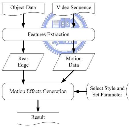
(12) automatically accomplish it. The system can produce various motion effects and effectively reduce the time for painting in cartoons.. 1.2 Overview Generally there are two purposes of motion effects: One is representing the direction of movement, and the other is setting off the atmosphere by contrast such as displaying the high-speed moving. For these purposes artists create various motion effects and we try to classify them and construct a proper procedure to draw them. The system flow chart is shown below.. Figure 1.2 Flow chart of the system First of all, the user inputs video sequence and objects data. There can be more than one object in a video sequence. In the next step, feature extraction, the system will find the contours of the objects and estimate the motion of them. According to 2.

(13) these data, we provide a default value to analyze the position of rear edge and decide whether the object should be applied motion effects or not. Then the system will output these data.. In the step of motion effects generation, user can choose which kind of effects will be applied and then change the parameters to accomplish different results until satisfied. Note that some effects can be used as a single stylistic element or they can be combined. So user may choose more than one effects. After the parameter setting, the system will complete the whole painting process.. Our contribution is that we extend the classification of motion effects, and try to find the sharing common linkage of them. Furthermore, we establish techniques to generate various motion effects even the objects have complicated shape and deformed in different frames. Users can easily obtain a desired motion effects through parametric control.. The remainder of this thesis is organized as follows. In Chapter 2 we review the related work of motion effects and cartoon style painting. Then we present the study and analysis of non-photorealistic motion effects in Chapter 3. In Chapter 4 and 5, we demonstrate the process and algorithm to generate various motion impressions. Chapter 6 shows the results and future research directions.. 3.

(14) Chapter 2 Related Works. Due to the physiology, persistence of vision, we can see afterimages when an object moves fast. In photography, if an object is moving during the exposure time, the result image of the object will be blurred. This effect is called motion blur. In animations, animators use different and simpler ways to accomplish this perception, such as speed-line. Unlike photorealistic motion effects, such as motion blur which is a well studied and established technique [8,9], non- photorealistic motion effects are rare studied. We demonstrate some related studies about style of non-photorealistic motion effects, stroke, and the automatic generation of motion in this chapter.. Cartoon can be regarded as a style of painting arts, and its painting style of motion effects is various. Strothotte et al. [10] proposed three stylistic techniques of sketch rendering to represent the movements of objects. Masuch and Stefan et al. [7,11] also proposed similar categories of illustrative moving elements, such as speed-lines and full or partial contour repetitions. They both show that these non-photorealistic motion effects used in animation are inspired from comic caricatures.. Although cartoon production has already transformed to use computers, 4.

(15) animators still want to shown the painting style using traditional cel animation. In order to simulate the hand-drawn pen stroke used in cel animations and comics, Hsu and Lake et al. [6,4] proposed similar approaches using the triangular slivers to simulate the style of speed-line. Strothotte et al. [11] proposed a sequence of quadrilaterals to simulate line-drawing. We proposed a method based on these two approaches but have a little enhancement.. In recent researches, the proposed approaches to simulate non-photorealistic motion effects need users to determine which vertices of an object require speed lines and the system will track the movement of vertices. Besides almost all of them only show one motion effect, the speed-line. Kawagishi et al. [5] proposed a method focused on one moving object to determine the position of painting motion effect automatically, which integrated two different kinds of motion effects. Their method has defects in dealing with the objects which have complicated contour and deformation between frame to frame. Besides if there are multiple objects in a frame how to judge which objects require to show motion effects.. 5.

(16) Chapter 3 Investigation of Animation. The word animation stems from the Latin word animare, which means to fill with life. In this sense, animations create the illusion of movement and bring still images to life. In this chapter, we discuss the painting skills and styles of stroke and motion effects in animations.. 3.1 Media of Cartoon Painting In traditional animation or comic painting, many kinds of painting instruments are used, such as color pencil, watercolor, crayon and so on. Generally, animators use pencils to draw the sketches, then use pen and ink to trace contours [12].. When painting effective lines, hand and pen need to leave paper slowly and steadily like the airplane takes off, and can not suddenly stop in the mid of painting a line. On the other words, the stroke can not get thinner suddenly, but slowly. The end of a line should be a long and thin triangle [1]. Strothotte et al. [11] show a example that a cartoon character with this style have remarkable change (Figure 3.1). 6.

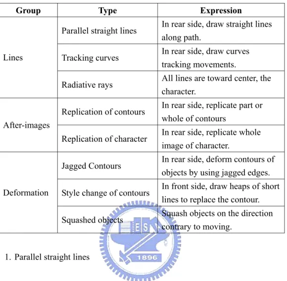
(17) (a). (b). (c). Figure 3.1 “The Little Worm” (a) The path for worm (b) The style that is applied (c) A cartoon character with style. 3.2 Classification of Motion Effects As mention before, animators take into account the different situations and use various expressions to present the movement of a character correspondently. Kawagishi et al. [5] classify these non-photorealistic motion effects into three groups. In the rest of this section, we discuss these motion effects in detail. Table 3.1 summarize this classification.. A. Lines. Effective lines are the simplest and most frequently used skill to present movement in cartoons and comics. Additionally, the skills are often applied to represent the emotion of characters. It can be further classified into three types: parallel straight lines, tracking curves, and radiative rays.. 7.

(18) Table 3.1 Classification of Non-photorealistic Motion Effects Group. Lines. Type. Expression. Parallel straight lines. In rear side, draw straight lines along path.. Tracking curves. In rear side, draw curves tracking movements.. Radiative rays. All lines are toward center, the character.. Replication of contours. In rear side, replicate part or whole of contours. Replication of character. In rear side, replicate whole image of character.. Jagged Contours. In rear side, deform contours of objects by using jagged edges.. Style change of contours. In front side, draw heaps of short lines to replace the contour.. Squashed objects. Squash objects on the direction contrary to moving.. After-images. Deformation. 1. Parallel straight lines. This technique is referred to as speed-lines and is usually drawn in the rear side of objects. The direction of lines is along the direction of movement. An example is shown in Figure 3.2 [11]. According to the density of line, the sense of speed is changed. If the lines are longer and denser, we will feel the speed is faster.. (a). (b). Figure 3.2 Parallel straight lines (a) Sparser and shorter lines. (b) Denser and longer lines 8.

(19) 2. Tracking curves. This technique is similar to previous one, but more faithfully represent the track of movement. Since the character does not only move along a straight line, the artist may use curves to represent the movement. The curves are also usually drawn in the rear side but not always parallel to each other. This skill usually use in the situation that moving track is longer. Figure 3.3 is an example of this skill [2].. Figure 3.3 An example of Tracking curves 3. Radiative rays. Whilst drawing this effect, artists need to decide a center region that is always a circle. Then they draw lines toward the center point but do not cover center region. This skill can be regard as speed-line. It is usually used when the moving direction is perpendicular to the image. For example, in Figure 3.4, the characters fall into a hole. Additionally, the skill is powerful to express shocked emotions.. Figure 3.4 Radiative rays (Magister Negi Magi) 9.

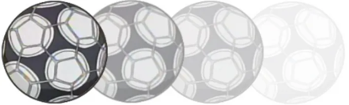
(20) B. After-images. This technique replicates images or contours between the positions in two different frames and is always drawn on the rear side of objects. It can be classified into two types: replication of contours or characters.. 1. Replication of contours. An example of this technique is shown in Figure3.5 [7]. The style of drawn part of the contours is more often used than the entire of them. The repeated part may get smaller and smaller.. (a). (b). (c). Figure 3.5 Replication of contours (a) Full rear edge (b) Gradually decreased rear edge (c) Full contours 2. Replication of character. This technique is often used in the situation that utilizing slow motion to emphasize fast moving. It always repeat entire of characters, but the color gets lighter and lighter as shown in Figure 3.6.. Figure 3.6 Replication of character 10.

(21) C. Deformation. We define the effects that cause the stroke style or the shape of objects changed are belong to this type. It consists of three types: jagged contour, style change of contours, and squashed objects.. 1. Jagged Contours. This technique uses jagged edges to deform the rear contours of an object as shown in Figure 3.7 [5]. Figure 3.7 Jagged contours 2. Style change of contours. This technique is drawing a lot of heaps of short lines to cover the contours of objects. The direction of lines stands on the direction of movement. It is usually drawn on the front contour of objects, as shown in Figure 3.8 [2].. Figure 3.8 Style change of contours 11.

(22) 3. Squashed objects. This technique is squashing objects along the contrary direction of movement and may be stretching objects along the direction of moving, as shown in Figure 3.9. This style of motion effect is always accomplished at the same procedure as character drawing. On the other words, the job of painting this effect does not belong to post-processing. According to this, we do not implement this effect in this thesis.. Figure 3.9 Squashed objects (Keroro Kunso). 12.

(23) Chapter 4 Feature Extraction. It is mentioned that animators always draw motion effects after they accomplish drawing characters and backgrounds. Besides the software used in animation painting generally has the concepts of layers. Characters and backgrounds are always painted in the different layers. On the other words, painting motion effects can be regard as a post processing, and the objects and film model in embryo are easily available. We use these data as inputs.. After users input data, we need to analyze it and obtain useful information. In this chapter, we describe feature extraction about motion estimation in Section 4.1 and rear and front edges in Section 4.2.. 4.1 Motion Estimation In painting of motion effects, motion direction is an important feature. Kawagishi et al. [5] proposed a method that estimates motion pixel by pixel. Since the objects in cartoon are always deformed or scaled in different frames, the situation which can use the method is very limited. In order to deal with this problem, we. 13.

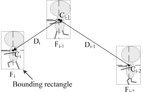
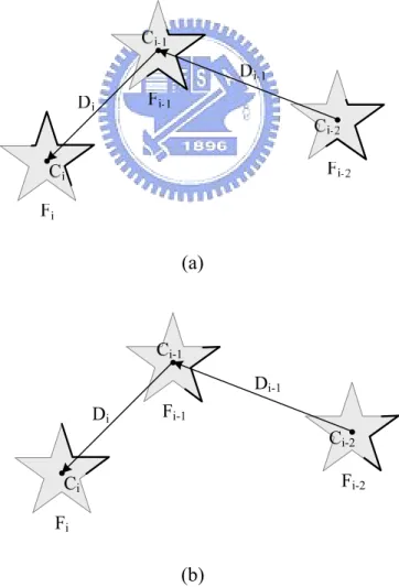
(24) proposed a simpler but useful technique to accomplish the motion estimation.. Motion impressions often represent the movement of the whole objects, rather than display the movement part of objects that may have corresponding deformation in different frames. For example, when a man is running, his legs have corresponding changes in different frames. If we want to represent that he is running fast by motion effects, we focus on the fast movement of the whole body rather then the fast moving legs. If we want to emphasize the fast movement of his legs, we can regard the legs as an independent object. According to this theory, we decide to estimate the movement of the whole object rather than the movement of each pixel.. First of all, according to the input objects, we construct the bounding rectangle of each object in each frame. At the same time, we can obtain the width, height, and center of the object. Then we use the movement of center in each frame to descide the movement of an object.. As shown in Figure 4.1, a character moves from Fi-2 to Fi (Fi means in the i-th. Figure 4.1 Motion direction 14.

(25) frame). After we construct the bounding rectangles of characters in each frame, we can obtain the position of centers, C which is the center of bounding rectangle. The direction of movement in the i-th frame, Di, can be derived from Ci – Ci-1. In the first frame, since there is not previous frame, we use the direction of the second frame as its direction.. In animation, there are often multiple objects in a frame. In order to judge which object needs to draw motion effects, we use a function to estimate: N. λL. ∑ Li i =2. N −1. N. + λS. ∑S i=2. i. N −1. ≥ εm. (4.1). Li is the moving distance from frame i-1 to frame i. On the other hand, Li is the length of Di, the vector of moving direction in the i-th frame. It can measure the movement of object in x and y direction. We sum the moving distance from the second frame to the last. Then we calculate the average of moving distance from frame to frame. N represents the number of frames.. Si is the estimator of scaling. Because the input data is 2D information, how to estimate the movement along the z direction becomes a difficult problem. After analyzing the 2D cartoon painting, we discover animators use scaling objects for the perception of moving along z direction. This painting technique is derived from linear perspective as shown in Figure 4.2. For example, if a character is running toward viewers, the character is getting bigger and bigger. Oppositely, if a character is running away from viewers, the character is getting smaller and smaller.. 15.

(26) Figure 4.2 Linear Perspective According this concept, we use the degree of scaling to estimate the movement in z direction:. Si =. Ai − Ai −1 (Wi × H i ) − (Wi −1 × H i −1 ) = Ai −1 Wi −1 × H i −1. (4.2). Wi and Hi are the width and height of bounding rectangle respectively in the i-th frame. Then we can derive the area of bounding rectangle, Ai, from the product of them. Si is defined as the scaling factor of areas between current and previous frame. To moving distance, we calculate the average of scaling factors.. Since these two estimators are estimated in different units, we use two weighting values, λL and λS, to modulate the influence of them. In detail, Li estimates moving distance by pixel, and the value is usually over tens. Si estimates movement by the percentage, and the value is always between 0 to 1. Then the influence of both estimators will not be ignored.. The parameter, εm, is the threshold for motion estimation. If the first term of equation (4.1) is over the threshold, it means the moving degree of object is large enough, and the object need to paint motion effects.. 16.

(27) 4.2 Rear Edges and Front Edges The most difficult problem in automatic generation of motion effects is location of these effects. By observation, we found most style of motion effects are painted behind the objects. If we can determine which part of contour belongs to rear, we can use the rear edge to be the basic positions for painting motion effects.. Kawagishi et al. [5] proposed a technique to detect rear edges. They use the positive of dot product between moving direction and the vector from current vertex to next to judge rear edges. Their method has a defect that when dealing with concave polygons the judgment of rear edge is wrong. Due to the characters in cartoon mostly have complex shapes, the algorithm only can deal with convex polygon is not enough. We proposed a novel method to detect rear edges.. First, according to the input objects, we analyze the contours of objects in each frame, and sort the vertices of the contour counterclockwise. Then we detect these vertices is front or rear in sequence.. We detect rear as shown in Figure 4.3. We use the information obtained in motion estimation. Di is the moving direction in ith frame, and Vi, j is the vector from center of objects to the point we detect, Pi, j, which means the jth point in ith frame. We normalize these two vectors, and if a vertex belongs to rear, it would conform to the inequality below:. Di ⋅ Vi , j ≤ cos θ. (4.3). 17.

(28) Ci-1 Di Pi, j. Fi-1. Vi, j. Vi, j+1 Ci Pi, j+1 Fi Figure 4.3 Detection of Rear Edges This method is very simple, and corresponds to our intuition. Users can obtain different length of rear edge through the parameter, θ. For example, in Figure 4.4 (a),. (a). Ci-1 Di-1 Di. Fi-1 Ci-2 Fi-2. Ci Fi. (b) Figure 4.4 An Example of Rear Edges: (a) θ = 90° (b) θ = 135°. 18.

(29) if θ is 90°, the rear edges of the object are the border parts. If θ change to 135°, the result is shown in Figure 4.4 (b). The lengths of rear edges will affect the region of painting motion effects. For example, if we want to paint the same number of speed-lines, the rear edge is longer, and the density of speed-line should be sparser. It result in different perception of speed.. Contrary to the rear edges, the points which do not belong to rear are front. So, after judging the rear edges, we also obtain the front edges.. 19.

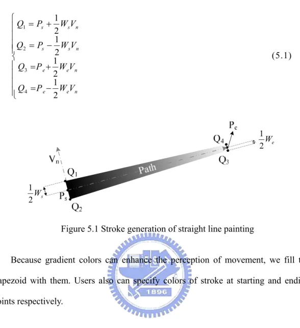
(30) Chapter 5 Generation of Motion Effects. In this chapter, we discuss how to generate motion effects as mentioned in Chapter 3. In Section 5.1, we describe the techniques of stoke generation. In the following sections, we demonstrate the generation of the three groups of motion effects which includes lines, after-images, and deformation.. 5.1 Stroke Generation In stroke generation, our purpose is to simulate hand-drawn pen stroke which get thinner slowly. We deal with painting straight lines and curves utilized in two different ways respectively.. In straight line painting, we generate stokes as shown in Figure 5.1. The path of stroke is from Ps to Pe. After user specified widths of a line, Ws and We, at starting and ending points respectively, we use a trapezoid to simulate the stroke. According to the normal direction of stroke, Vn, we can obtain four vertices of trapezoid:. 20.

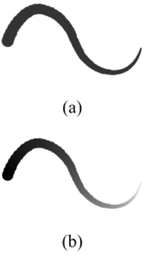
(31) 1 ⎧ ⎪Q1 = Ps + 2 WsVn ⎪ 1 ⎪Q2 = Ps − WsVn ⎪ 2 ⎨ 1 ⎪ Q3 = P e + WeVn 2 ⎪ 1 ⎪ ⎪⎩ Q4 = P e − 2 WeVn. (5.1). 1 We 2. 1 Ws 2. Figure 5.1 Stroke generation of straight line painting Because gradient colors can enhance the perception of movement, we fill the trapezoid with them. Users also can specify colors of stroke at starting and ending points respectively.. In curve painting, we generate stokes as shown in Figure 5.2. The path of stroke is from Ps to Pe. We draw a sequence of circles to generate the stroke. The centers of circles are points positioned on the curve. The diameters gradually decrease from Ws to We, widths of stroke at starting and ending point respectively.. Figure 5.2 Stroke generation of curve painting 21.

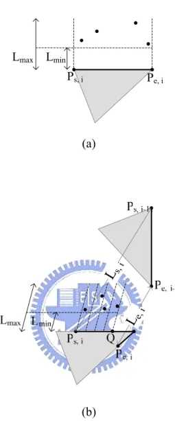
(32) Like the straight line painting, we implement gradient color for the curve strokes. Figure 5.3 shows the resulting stroke which applied single or gradient color.. (a). (b) Figure 5.3 Curve painting (a) Color: black (b) Color: from black to white. 5.2 Motion Effects: Lines It has been mentioned that there are three type of motion effects belong to the group of lines. We discuss their generation in this section.. 5.2.1 Parallel Straight Lines Since this type of motion effect is always drawn on the rear side, we use the position of rear edge as the basic starting points to generate the motion effect. Users need to specify the number of lines, and the minimum and maximum distances from rear edge, Lmin and Lmax respectively. We propose two methods to generate the position of starting points for line painting, as shown in Figure 5.4. The parameter, Ps, i, is the starting point of rear edge in i-th frame, and Pe, i is the ending point. The bolder lines are rear edges.. 22.

(33) Lmax. Lmin Ps, i. Pe, i. Le. ,i. Ls. ,i. (a). (b) Figure 5.4 The generation of starting points (a) Random (b) Regular random The first method is shown in Figure 5.4 (a). If the number of lines is 4, we randomly choose 4 points on the rear edge. The starting points are these points shift between Lmin and Lmax along the moving direction.. The other method is shown in Figure 5.4 (b). When animators utilize the motion effects of straight lines or curves to represent the movement, they often draw lines focused on some parts. For example, when they represent the movement of rotation, they draw lines focused on the part whose moving distance is longer. According to 23.

(34) this, we propose this method by considering the difference of moving distance between starting and ending points of rear edges. After users specify the proportional length of rear edge, R, we can derive the point Q:. ⎧ I ⎛ P ⎞ + R , if L ≥ L ⎪ ⎜ s, i ⎟⎠ s, i e, i I (Q ) = ⎨ ⎝ ⎪ I ⎛⎜ P ⎞⎟ − R , if L < L s, i e, i ⎩ ⎝ e, i ⎠. (5.2). I(Q) means the index number of the point, Q. We obtain new groups of candidate points from Ps, i or Pe, i to Q to generate the starting position for painting lines. Then we divide these vertices into equal parts. The number of division is equal to the number of lines. We randomly select a point on the rear edge in each part and shift the point between Lmin and Lmax along the moving direction. The resulting point is the starting point for painting lines.. After obtaining all starting points for painting lines, we derive ending points according to lengths and the moving direction of the object. Users need to specify the maximum and minimum length of lines, and we determine the final length randomly between them. The point shift final length from the starting point along the reverse direction of movement is the ending point.. After obtaining both starting and ending points, we use the stroke for straight line painting as mentioned in Section 5.1 to generate this motion effect.. 5.2.2 Tracking Curves As mentioned before, painting the motion effect of tracking curves is quite similar to painting the motion effect of straight lines. Starting points are also 24.

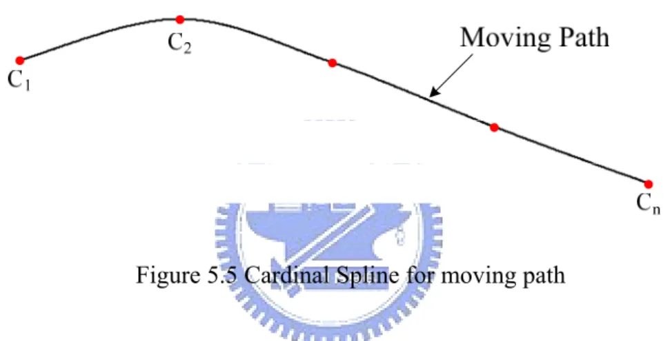
(35) generated by the same approach.. However, in order to simulate the continuous path of movement from discrete moving position, we use Cardinal Spline to simulate the path. Since Cardinal Spline is an interpolation curve, we may select central points of objects, C, as the control points. Then we may adjust the smoothness of curve by parameter α. Figure 5.5 shows an example to represent the moving path by using Cardinal Spline, where α= 2.0.. Figure 5.5 Cardinal Spline for moving path In Figure 5.6, we demonstrate the method to generate the paths for the motion effect of tracking curves. The parameters, i, j, k, represent the j-th control point of the k-th tracking curve in the i-th frame. After the generation of starting points, Qi, k, j, we can derive the vector, Vi, k, from the central point to the new starting point. Then, the other control points of a tracking curve, such as Qi, k, j+1 and Qi, k, j+2, are derived from shifting the central points in each frame. After obtaining all control points, we can accomplish the new path, such as path k, using Cardinal Spline. The number of tracking curves and the number of referring frames can be specified by users.. 25.

(36) Figure 5.6 Paths generation of tracking curves Since the maximum length of path is determined by the number of referring frames, users need to give the maximum and minimum percentages to specify the range of length. And we randomly generate the final length in the range. Finally, we apply the stroke for painting curve, as mentioned in Section 5.1, to generate this motion effect.. 5.2.3 Radiative Rays Unlike other motion effects in the group of lines, radiative rays do not use the position of rear edge as the basic position to draw the motion effect. As animators paint this effect, we begin the generation of radiative rays from determining the circular center region. The diameter of the circle is the maximum between the width and the height of the bounding rectangle. The center of the circle is the center of the bounding rectangle. Then we need to determine the direction and length of each ray for painting.. 26.

(37) Users need to specify the parameters as follows: The number of lines is determined by the number of segments, M, and the maximum number of rays in each segment. Rmin and Rmax are the percentages of shifting distances, and they determine the shifting ranges of starting and ending points for each ray respectively. Lmax is the maximum length of rays. NL is the number of layers. The parameters, θs and θe, are starting and ending angles respectively.. Since there may be multiple layers of radiative rays, we need to determine the maximum length of each layer. We determine the length as shown in Figure 5.7 (a). In this example, the number of layers, NL, is two. Since the length of layers should be increasing from center, we determine the length of each layer, such as L1 and L2, as follows:. Lk = Lmax ×. k. (5.3). NL. ∑u u =1. The parameter, k, means the k-th layer. Since the rays in each layer should be distance away, the maximum length of rays in each layer does not equal to the length of layer. We use a parameter, RL, which is the percentage of length, to determine the maximum length of rays in each layer as follows: Lk′ = RL × Lk. (5.4). L'k means the the maximum length of rays in the k-th layer. After obtaining lengths, we can define the region to paint radiative rays, as the grey region shown in Figure 5.7 (a). The basic starting points of rays are located on the bounding circumferences which is black in the grey region.. 27.

(38) L2 L1. Ci. L'1 L'2. Lmax (a). L'1 PM. .... P2 P1. Ci. θlimit. P0. L'1*Rmin L'1*Rmax (b) Figure 5.7 Generation of radiative rays: (a) lengths of rays (b) directions and the basic positions We determine the directions of rays as shown in Figure 5.7 (b). Since the directions of rays can be defined as (cosθ, sinθ), we regard the problem of direction generation as angle generation. In this example, θ s and θ e are 0 ° and 90 ° respectively. On the other words, the directions of rays range from 0° to 90°. Then, we equally divide the range of angle into M segments, and Pj is the partition point. We use Pj as the center of each segment. Then randomly generate angles between a limitative angle, θ limit. The number of angles in a segment can not over the 28.

(39) maximum number specified by users. After the generation of angles, we not only obtain the directions of rays, but also derive the number of rays. The basic starting and ending points of radiative rays are the intersection points of the circumferences in each layer and the vectors of directions.. According to the percentages, Rmin and Rmax, we can obtain the corresponding ranges to generate starting and ending points of rays in each layer, as shown in Figure 5.7 (b). Then we randomly shift the basic starting and ending points to the corresponding regions, and generate each ray using the stroke for straight line painting, as mentioned in Section 5.1.. 5.3 Motion Effects: After-image In this section, we demonstrate the generation of two motion effects which belong to the group of after-image. They are replication of contours and characters.. 5.3.1 Replication of Contours In order to generate this motion effects, users need to specify these parameters: Rmin and Rmax are the minimum and maximum percentages of shifting distances respectively. M is the number of replications.. We determine the shifting distances of replications as shown in Figure 5.8. Li means the moving distance of the object from frame i-1 to frame i. The minimum shifting distance, Lmin, is derived from the product of Li and Rmin. The maximum shifting distance, Lmax, is derived from the product of Li and Rmax. We equally divide the distance from Lmin to Lmax into M parts. Each shifting distance of replications is 29.

(40) from Ci to Pk, where k is the k-th replication.. Figure 5.8 Ranges of shifting distances for replications For the replications of the entire rear edges, we shift rear edges along the inverse direction of movement and repaint them. For the replications of the decreasing rear edges, we linearly decrease the lengths of rear edges according to the function as follows:. LRk =. k M. ∑k. ⋅ LRentire. (5.5). k =1. LRk means the length of rear edge in the k-th replication, and LRentire is the entire length of rear edge. We shorten the rear edge from two ends, and use the stroke for curve painting, as mentioned in Section 5.1, to generate this effect. We set the center of each repainting rear edge as the starting point of a curve, and the ending point of each repainting rear edge as the ending point of a curve. The resulting curve will get thinner from the center to the two ends.. 5.3.2 Replication of Characters The generation of this motion effect is similar to the replication of contours. We apply the same method to determine the shifting distances and directions. The 30.

(41) difference is that we need to redraw the entire characters in this motion effect.. In order to generate the replications which are getting paler and paler, we increase the transparency of the character in each replication. Although changing the intensity also can obtain the effect getting paler and paler, the replications with opaque characters will cover the original background. Due to this, we choose to change the transparency rather than the intensity.. Besides, because the original character should be much clearer than the replications, we use a function to increase the speed of getting paler. When the transparency is from 0 to 1, the equation is as follows:. ηk = 1 −. (M − k ) 2 M2. (5.6). The parameter, ηk, means the transparency in the k-th replication, and M is the number of replication. When the transparency close to 1, the replication is more transparent.. 5.4 Motion Effects: Deformation In this section, we demonstrate the generation of two motion effects which belong to the group of deformation. They are jagged contours and style change of contours.. 5.4.1 Jagged Contours In this type of motion effect, we propose three methods to jag contours of objects.. 31.

(42) These methods use different ways to determine which points need to shift, and the corresponding shifting distance, as shown in Figure 5.9.. (a). (b). (c) Figure 5.9 Generation of jagged contours: (a) Regular intervals (b) Determination of intervals and shifting distances with considering the movements (c)Disconnected jags. 32.

(43) We specify the parameters used in this section as follows: . . . . . . Ps, i and Pe, i are the starting and ending points of rear edges in the i-th frame respectively. Lmin and Lmax are the minimum and maximum shifting distances from the rear edge respectively. Ldis means the shifting distance between them. Shifting distances determine the degree of jagging. Mt means the number of jags. Ms is the number of segments. Mj means the maximum number of jags in each segment. The parameter, k, means the k-th segment, and k is from 0 to (Ms -1). NSk is the number of jags in the k-th segment. LIk represents the interval which is the range to randomly determine which points need to shift. LHk represents the interval to limit the shifting distances of high points in jagged contours. LLk represents the interval to limit the shifting distances of low points in jagged contours.. The first method is shown in Figure 5.9 (a). After users specify the number of jags, we equally divide the rear edge into (2* Mt -1) segments. The interval of each segment is equal. We randomly choose a point in each interval, and shift them along the inverse direction of the movement. The odd points shift the distance which randomly determined between Rmin and Rmax. The even points shift the distance which randomly determined between 0 and Rmin. Then we can derive a new jagging contour from linking these points.. The second method is shown in Figure 5.9 (b). Sometimes, animators determine the degree of jagging according to the moving distance. For example, when waving a stick, the part of stick which is farther from the character move more distance. Animators often jag the part of stick more heavily. According to this, we decide the interval of each segment as follows: 33.

(44) NS = k. (k + 1) × M MS. ∑u. t (5.7). u =1. L r LI = k 2 × M × NS s k. If |Ps, i – Ps, i-1| ≧ | Pe, i – Pe, i-1|, the k-th segment starts from Ps, i to Pe, i. On the contrary, the k-th segment starts from Pe, i to Ps, i. After users specify the parameters, Mt and Ms, we can determine the number of jags and the interval of each segment. Then, we randomly choose a point in each interval, and shift it along the reverse direction of the movement. The intervals of shifting distances in each segment are specified as follows:. (. ). (. ). ⎞ ⎛ M −k 2 ⎞ ⎛ M − (k + 1) 2 ⎟ ⎜ s ⎟ ⎜ s < LH ≤ ⎜ ×L ⎟+L ×L ⎟+L ⎜ min dis k dis min (5.8) ⎟ ⎜ M2 ⎟ ⎜ M2 s s ⎠ ⎝ ⎠ ⎝ 0 < LL ≤ L k min. Then, as the previous method, we can derive the new jagging contour from linking these points.. In order to generate disconnected jags, we propose the third method, as shown in Figure 5.9 (c). We equally divide the length of rear edge into Ms parts. Then users can specify a percentage to narrow the interval. After determining the interval, the starting and ending points of jagged contours for each set are determined as the two ending points of each interval. The others points which need to shift are randomly chose in the interval. The interval of shifting distance in each segment is specified as follows:. 34.

(45) L × Percentage < LH ≤ L max 1 max L < LH ≤ L × Percentage min max k 0 < LL ≤ L min k. (5.9). Then, as the previous method, we shift points along the inverse direction of the movement, and derive the new jagging contour from linking these points.. 5.4.2 Style Change of Contours In this motion effect, we replace the points on front edge with short lines. Users can specify the maximum and minimum lengths of lines, and the interval between each short line. Then, we draw the short lines according to the direction of the movement, as shown in Figure 5.10. Ps and Pe are the starting and ending points of the rear edge.. Ps. Pe Interval. Figure 5.10 The generation of style change of contours. 35.

(46) Chapter 6 Implementation and Results. In this chapter, we demonstrate our implementation results. Tables 6.1 and 6.2 show two results of motion estimator, as mentioned in Section 4.1. Figures 6.1 and 6.2 display the sample shots of estimation respectively. In these tables, λL is the weighting value of moving distance, λS is the weighting value of scaling, and εm is the threshold. The forth column refers to the judgments of painting motion effects. If the value is “YES”, it means the object needs to paint motion effects. On the contrary, if the value is “NO”, it means the objects dose not need to paint motion effects. In Figure 6.1, the object one and the object two are the left and right shoes respectively. In Figure 6.2, the object one is the girl with orange hair on the right-hand side, and the object two is the girl with black hair on the left.. Figure 6.1 The first example for motion estimation (School Rumble).. 36.

(47) Table 6.1 The result of motion estimation for Figure6.1. λL 1.0. λS 1.0. εm. Is Draw. Object 1. Object2. 80. YES. YES. 90. NO. YES. 100. NO. NO. Figure 6.2 The second example for motion estimation (Hime). Table 6.2 The result of motion estimation for Figure6.2. λL 0.8. λS 1.5. εm. Is Draw. Object 1. Object2. 40. YES. YES. 55. YES. NO. 65. NO. NO. The first results of motion effect which includes straight line and curve tracking are shown in Figures 6.3 to 6.6. The target object is the suitcase carried by the boy who wears red clothes. Figure 6.3 (a) shows the input data, and the red lines in Figure 6.3 (b) are the results of rear edges with the parameter, θ=90°.. 37.

(48) (a). (b). Figure 6.3 Rear edges (One Piece) (a) Input data (b) Results Figures 6.4 and 6.5 are the motion effects of straight line applied different position generator. In Figure 6.4, we use the generator without considering the movements. The basic starting points of lines are randomly distributed on the entire rear edge. In Figure 6.5, since we use the generator with considering the movement, the starting points of lines are mainly distributed on the rear edge of where the moving distance is longer. Figure 6.6 is the motion effect of curve tracking applied the position generator with considering the movement.. 38.

(49) Figure 6.4 Straight lines applied the random position generator (One Piece). 39.

(50) Figure 6.5 Straight lines applied the position generator with considering movement (One Piece). 40.

(51) Figure 6.6 Curve tracking applied the position generator with considering movement (One Piece).. 41.

(52) Figure 6.7 is the result which shows the motion effects of radiative rays. The target object is the group of people on the right bottom corner. The number of layers is two, and the range of angle is from 65° to 165°.. Figure 6.7 Results of radiative rays (School Rumble). 42.

(53) Figures 6.8 to 6.11 show different styles of motion effects in the group of after-image. The input data and the rear edges with the parameter, θ=75°, are shown in Figure 6.8 (a) and Figure 6.8 (b) respectively. The target object is the ladle. The replication of contours without decreasing is shown in Figure 6.9, and the result with decreasing is shown in Figure 6.10. Figure 6.11 shows the replication of images.. Figure 6.8 Rear edges (Keroro Kunso) (a) Input data (b) Results. 43.

(54) Figure 6.9 Replication of rear edges without decreasing (Keroro Kunso). 44.

(55) Figure 6.10 Replication of rear edges with decreasing (Keroro Kunso). 45.

(56) Figure 6.11 Replication of images (Keroro Kunso). 46.

(57) Figures 6.12 to 6.14 show the motion effects of jagging contours applied different methods. The target object is the bat. The result with regular interval and length is shown in Figure 6.12. The result applied the interval and length with considering the moving distance is shown in Figure 6.13. Figure 6.14 shows the result applied disconnected jags.. Figure 6.12 Jagging contours with the regular interval (Honey and Clover) 47.

(58) Figure 6.13 Jagging contours applied the interval and length with considering movements (Honey and Clover). 48.

(59) Figure 6.14 Disconnected jags (Honey and Clover). 49.

(60) Figure 6.15 shows the result of the motion effect, style change of contours. The target object is the ball. We apply the effect to the entire contour of the ball.. Figure 6.15 Style change of contours (Magister Negi Magi). 50.

(61) Finally, Figure 6.16 shows the result which combines the replication of contours and the curve tracking. The target object is the suitcase carried by the boy who wears red clothes.. Figure 6.16 Result which combines two styles of motion effects (One Piece). 51.

(62) Chapter 7 Conclusions In this thesis, we analyze the non-photorealistic motion effects in cartoon, and classify these motion effects into three groups. According to the analysis of animations, we propose a method to estimate the movement of objects. We find most motion effects can be generated based on the rear edges. We propose algorithms to synthesize different styles of motion effect. In our system, users can easily generate various motion effects parametrically. Besides, with our help, animators can save time to generate these motion effects.. However, there are still issues to enhance our system in the future. First, the motion estimation has some limitations. For example, the objects moving track may approximately follow a curve. However, it is actually moving slightly out of the track. It will result in the tracking curve with many bends, or the judgments of moving directions do not follow a smooth curve. In the future, it might be able to use the Linear Regression to modify the moving track. Second, we find that animators sometimes apply the motion effects of deformation not only to the contours, but also to the edges in the object. We can consider this situation in the future. Third, we can improve the motion effect, style change of contours, since the results seem too regular. Fourth, users need to choose the style of motion effects in our system. We can. 52.

(63) automate this procedure according to the analysis of moving velocity. Since different motion effects should be suitable for different moving speeds. Besides, we may integrate our system with Flash to produce animation. Since there is a layer concept in the format of Flash, we may easily get input, object data and video sequence. And we can apply different motion effects to each object.. 53.

(64) Reference. [1]. 日本漫畫技法研究會，《卡通漫畫技法百科》，中國青年出版社，2003 年出版。. [2]. 林晃，《格鬥的畫法》，萬里機構．明天出版社，2002 年出版。. [3]. 藤堂良，《鋼筆與色調漫畫技法》，台灣珠海出版社，1997 年出版。. [4]. Siu-Chi Hsu, and Irene H. H. LEE. “Drawing and Animation Using Skeletal Strokes”, Proceedings of ACM SIGGRAPH, 1994, pages 109-118.. [5]. Yuya Kawagishi, Kazuhide Hatsuyama, and Kunio Kondo. “Cartoon Blur: Non-Photorealistic Motion Blur”, Proceedings of the Computer Graphics International, 2003.. [6]. Adam Lake, Carl Marshall, Mark Harris, and Marc Blackstein. “Stylized Rendering. Techniques. For. Scalable. Real-Time. 3D. Animation”,. Non-Photorealistic Animation and Rendering, June, 2000.. [7]. Maic Masuch, Stefan Schlechtweg, and Ronny Schulz. “Depicting Motion in Motionless Pictures”, Proceedings of ACM SIGGRAPH, 1999.. 54.

(65) [8]. Nelson L. Max, and Douglas M. Lerner. “A Two-and-a-Half-D Motion-Blur Algorithm”, Proceedings of ACM SIGGRAPH, July 1985.. [9]. Michael Potmesil and Indranil Chakravarty. “Modeling Motion Blur in Computer-Generated Images”, Proceedings of ACM SIGGRAPH, volume 17, 1983.. [10] Thomas Strothotte, Bernhard Preim, Andreas Raab, Jutta Schumann, and David R. Forsey. “How to Render Frames and Influence People”, Proceedings of EuroGraphics, pages 455-466, 1994.. [11] Thomas Strothotte, and Stefan Schlechtweg. “Non-Photorealistic Computer Graphics”, Morgan Kaufmann, 2002.. [12] Richard Taylor. “Encyclopedia of Animation Techniques”, Running Press Book, 1996.. 55.

(66)