North-Holland
sing Hsu, Rong-Hong Jan, Uu-Che Lee and Chun-Nan
Department of Information and Computer Science, National Chiao Tung University, Hsinchu 30050, Taiwan, ROC
Maw-Sheng Chern
Department of Industrial Engineering, National Tsing Hua University, Hsinchu 30043, Taiwan, ROC
Communicatect by K. Ikeda Received 7 January 1991 Revised 1 April 1991
Keywords: Data structures, design of algorithms, minimum spanning trees
1. uction
In many applications, the network designer may want to know which edges in the network are most important to him. If these edges are removed from the network, there will be a great decrease in its performance. Such edges are called the most vital edges in a network. Several papers [1,2] have been presented to find the most vital edges. However, they are only concerned with the effect of the maximum flow or the shortest path in the net- work. In this paper, we will consider the effect of a minimum spanning tree in the network.
Most graph-theoretic terms used in this paper are standard (e.g., [3]). Here, we limit ourselves to defining the most commonly used terms and those that may produce confusion. G = (V, E) is called a graph if V is a finite set and E is a subset of ((0, b) I a f b9 (a, W is an unordered pair of I/’ }. We say V is the vertex set of G, E is the edge set of G. Let p=(VI and q=IEJ. Let E be a subset of E. We use G - E to denote the graph G’ = (V, E - E). In particular, we use G - e and G + e to denote the graph G - (e} and G + {e}, respectively. Craph H = (V ‘, E ‘) is called a sub-
graph of G if V’ G V and E’c En (V’x V’). A
subgraph H = ( V ‘, E ‘) of G with V’ = V is called a spanning subgraph of G. A spanning tree of G is a connected spanning subgraph of G that contains no cycles.
A weighted graph is a graph G = (V, E) with a weight w(e) assigned to every edge e in E. The
weight of a spanning tree T, w(T), is defined to be
the summation of w(e) for all e in T. A spanning tree T in G is called a minimum spanning tree if
w(T) < w(T’) for all spanning trees T’ in G. Minimum spanning trees have many applications in network design, VLSI, geometric optimization and so on. There are two best-known algorithms used in finding the minimum spamning tree in a weighted graph. One is Kniskal’s algorithm [4] and the other is Prim’s algorithm [5]. It is known that Kruskal’s algorithm takes O(q log q) time whereas Prim’s algorithm takes Q( p2) time.
Let g(G) denote the weight of a minimum spanning tree of G if G is connected; otherwise, g(G) = 00. An edge e is called a most vital edge (MVE) in G if g(G-e)>,g(G-e’) for every edge e’ of 6. The problem of finding such an edge is called the I-MVE problem. Two al-
Volume 39, Number 5 INFORMATION PROCESSING LETTERS 13 September 1991
gorithms with time complexities O(q log 4) and 0( p2) are presented for solving the l-MVE prob- lem in this paper.
2. Some interesting pro
Throughout this paper, we assume that the costs of edges in G are different. With this as- sumption, the minimum spanning tree in G is unique. A naive way to find the most vital edge in G is finding g(G - e) for each edge e in E bv applying Kruskal’s algorithm. The most vital edge in G is thus easily obtained. However, this method takes 0(q2 log 4) time. We may reduce the time to 0( pq log q) once we have the following lemma:
mma 1. Let TG be the minimum spanning tree of G. Then, the most vital edge of G is one of the edges in TG.
oaf. It is clear that g(G - e) > g(G) if the edge
e is in TG. Let e * be the most vital edge. If e* is not in TG, then To is a spanning tree of G - e *. This implies that g( G - e * ) = g(G). There is a contradiction. Hence, the most vital edge of G must be one of the edges in TG. 0
With Lemma 1, the most vital edge of G is in its minimum spanning tree To. Thus, only 1 TG 1 =
p - 1 edges are considered and the time complex-
ity of the above naive method can be reduced to 0( pq log q). We need the following discussion to further reduce the time complexity.
Let &? be the set of all edges in TG and B = E - 3. Let e = (c, b) be an edge in B and a =
vO, v],..., vk = b be the path with endpoints a and b in To. For each Y = (a, b), we define an edge set
R, that contains all edges in path a = vo, v,, . . . , ok = b. Then for e’ E &!, we define the edge sets
R,p as containing all edges e such that e’ E R,. Let f (e’), where e’ E 52, be the edge e in B such that w(e) = min{ w(e”
j
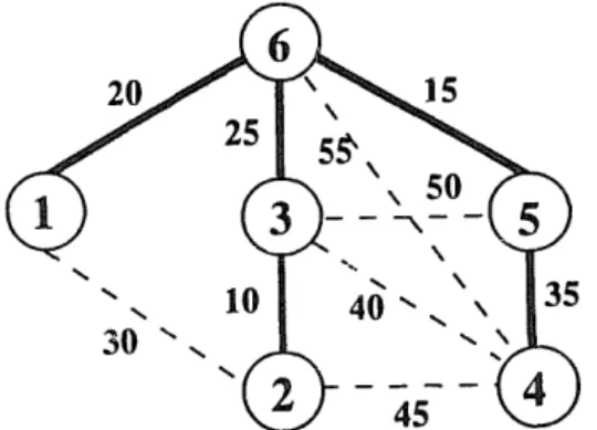
1 err E 8.f). For example,Fig. 1. Graph G.
the bold edges in Fig. 2 show the minimum span- ning tree of the graph G given in Fig. 1. Then, R(1.2, = ((2, 3), (3,6), (6, l)} 3 R (3.4) = ((39 a (69 99 (59 4)), R (2.4) = ((2, 3), (3, 6), (6, 5), (5, 4>}, R (3.5) = ((39 a (69 w and R (4.6)= (t4, 5), c5, 6)>-
Since (2, 3) E Ro2, and R(2,4,, the edge set R,,,, = {(1,2), (2, 4)). Obviously, f((2, 3)) = (1, 2).
mma 2. If e is in L?, then TG_e= TG- e +f(e). Hence w(T,_,> = w(T,) - w(e) + w(f(e)).
oaf. The proof is obtained by applying Kruskal’s algorithm on G and G - e. Without loss of gener- ality, w(e,) < w(e,) < l . . < w(e,) is assumed.
Kruskal’s algorithm [4] initializes the spanning
forest FO of G with no edge. At each iteration i, check if E__, U { e, } is acyclic or not. If e_ 1 U { e, } is acyclic, then set 6 = F, _ 1 U { e, }. Qther- wise, set 6 = I;;_,.
Let E and El_’ be the intermediate spanning forests obtained by applying Kruskal’s algorithm on G and G - e, respectively Let e = ej and f(e) = eh. Then j c h, otherwise eh is an edge of To. Thus, F’ = Fk if k <j. Since ek is the edge with w( e,) = min{ w( e”) 1 e” E R,}, we have F’ = F,-e,if j<k<h-1; and Fk)=Fk-e+f(e)if
kzh-1. Hence TG_e=TG-e+f(e). •I The edge f(e) is called the entering edge with respect to the leaving edge e. With Lemma 2, we may easily compute the most vital edge once we know the entering edge f(e), for every e E C& In the following, there are some properties about the trees that will be used later. Let T be a spanning tree of G. We may pick any vertex of T as a root and label the vertices of T from 1 to p in post- order. Thus, each vertex can be identified by its postordered number. All edges of T can be written as ( u, p( u)), where v is a nonroot node and p(u) is the parent of u. Let us regard every vertex as a descendant of itself. Then, we have Lemma 3.
Lemma 3. If e = ( u, p( 0)) is an edge of T, then f ( e ) must be an edge joining a vertex of a descen-
dant of v to a nondescendant of v.
3. An O(q log q) time algoait for the problem
The main idea of the algorithm presented in this section is to find the leaving edge set f - ‘(e ‘) for every e’EE- 1(2. Then, we apply Lemma 2 to compute the most vital edge in G.
lgorithm 1
Step 1. Apply Kruskal’s algorithm to find the minimum spanning tree TG of G = (V, E). Let Q be the set of edges in TG. Sort the edges in set B= E-L?= {e,, e2 ,...,
eq-p+l } in terms of their weights and
w(e,) < w(e2) < -- < w(eq_+,) is as- sumed. Let ( v.~, u,) = e,.
Step 2. Find the leaving edge set f -‘(e,y), f - ‘(e,) c I& for entering edges e,, s = 1. 2,. . . , q - p + 1, as follows.
2.1. Let F, = 0. Let R,$ be the set of all edges in the unique path from the vertex u, to u, in TG.
Step 3.
2.2. Set f-‘(e,)=R,, - F,_, and F,=
F,_,Uf-‘(e,),s=l,2 ,..., q-p+l.
For each edge e in TG, compute w(T~_~) = w(TG) - w(e) + w(f(e)). Find the edge e* such that w(T,_,*j = max{ w(TG_e) lthe edge e is in TG}.
By Lemma 2, it is clear that f(e) = e, for all edges e in the unique path from the vertex ui to u1 in TG. In general, f(e) = e, for all edges e in the unique path from the vertex u, to u, but not in
lJf=\ f -‘( ej). Thus, Step 2 finds f -‘( e,) correctly. We illustrate Algorithm 1 via the example in Fig. 1. Step I finds the minimum spanning
shown in Fig. 2. In Step 2, we find the edge sets f ‘( e,), for entering edges (e,, e2 ,...,e4-p+l ) =
((1,
2),
(3,4), (2,4), (3, 5), (476)) as follows: f -‘((l, 2)) = ((2,3), (3,6), (1,6))9 f -‘((3,4)) = ((4, 5), (5,6)),f -‘((2,4))
=o, f -‘((3,5)) =o, and f -‘((4,6)) =fl. Step 3 computes ( ( w 7&2.3Jr w(TG-(3.6J, w(G-~l.6J. 4 TG-(4.5) ), w(T,-f5.6, 0 = (125,110,115,110,130)and then finds the l!NE e* = (5, 6).
tree Tc leaving
Now, we describe the time complexity of Al- gorithm 1. Obviously, Steps 1 and 3 take
Volume 39, Number 5 INFORMATION PROCESSING LETTERS 13 September 1991
0( 4 log q) and O(p) time, respectively. At Step 2.1, the unique path from vertex u, to u,~ can be determined as follows. Let vertex q be the root of
T(-. Define the depth of a vertex c, denoted as
l(u), in TG is the distance of v from the root v,. (All edges have distance 1.) Search from vertex I-J* and u, to root v,, respectively. Start with the greater depth vertex and stop when a common ancestor vk is found. Then the unique path from the vertex u.~ to u, is obtained. With this imple- mentation, Step 2 takes 0( pq) time. Thus, the total time for Algorithm 1 is 0( pq). However, we may use the data structure UNION-and-FIND [6] on disjoint sets to reduce the time to O(q log q).
Step 2 of Algorithm 1 can be modified as follows by introducing the operations FIND(i) and UNION( i, j). The operation of FIND(i) is to determine the root of the tree containing ele- ment i. UNION(i, j) requires two trees with roots
i and j to be joined and assigns the vertex with the smaller depth among i and j as the root of the resultant tree.
Step 2. For s = 1, 2,. . . , q - p + 1, use the follow- ing procedure to find the leaving edge set
f -‘w
2.1. 2.2.
2.3.
Let (Q, u,) = e,. Let x = FIND( v,) and y = FIND( ~1,).
(Search from vertex x and JJ to root u respectively. Start with greater depth vertex.) If I(x) > I( ~9, then set u = z. Otherwise set u =y. Set z = p(u). Assign the edge (u, z) to edge set f -‘(es). Set z, = FIND(z) and process UNION(z,, u). If Z(x) > I( J), then set z, = x. Otherwise, set z, =y.
(Stop when a common ancestor uA- is found.) If x =y, then a common ancestor is found and go to Step 2 for next s. Otherwise, go to Step 2.2.
or
In this section, we present an gorithm to find the most vital ed graph. The input form is the
]w(i,
_iN
,..,
=I.2
. . . p-
We assume w(i, j) = 00 if there is no edge to connect vertexes i and j, and also assume w(i, i) = 00 for all i.Step 1.
Step 2.
Step 3.
Apply Prim’s algorithm to find the mini- mum spanning tree TG of G. Then, for all edges (i, j) in TG, set w(i, j) = co.
Pick any vertex u as the root of TG. Let tree T, denote the subtree of TG with root
i. Process the following procedure for each vertex i of ;4;; in postorder.
2.1. If vertex i is a leaf node, then set
c(i, j) = w(i, j), j = 1, 2,. . . , p. 2.2. If vertex i is not a leaf node with
child nodes i,, i,, . . . , i,, then set c( i, j) = min{ hp( i, j), c(i,, j), c(i,,
j),...,
c(i,, j)>, j = 1, 2,.. ., p.2.3. Find c( i, j* ) = min{ c( i, j) 1 vertex j is not in subtree q } and set f((i,
p(i)))=(j*, k), with w(j*, k)=
c(i, j*).
For each edge e in TG, compute w( TG_e) = w(TG) - w(e) + w(f(e)). Find the edge e* such that w(T,_,,) =
max{ w(TG_J 1 the edge e is in TG}.
Obviously, Algorithm 2 correctly computes f(e)
for every edge e in TG. Hence, we can easily compute the most vital edge in G. We also il- lustrate Algorithm 2 by using the example in Fig. 1. The input matrix is
Observe that it takes O(q) number of UNI and O(q) number of FIND in the procedure tree- expansion. The total time complexity in Step 2 is O( q - a( p, q)). Thus it takes 0( q log q) time in the modified Algorithm I.
cc 30 00 00 oc 20 30 00 10 45 00 00 00 10 00 40 50 25 Cc 45 40 00 35 55 2”o 00 00 50 25 55 35 15 00 15 00 280
Step 1 finds the minimum spanning tree TG shown in Fig. 2 and updates the weighted matrix as follows: oc 30 00 00 00 00 30 00 00 45 00 00 00 00 00 40 50 00 00 45 40 00 00 55 00 00 50 00 00 00 00 00 00 55 00 00
In Step 2, we pick vertex 6 as the root and find the entering edges f((i, p(i))), i = 1, 2,. . . ,5. For ex- ample, vertex 1 is a leaf node and then
(~(1, l), c(l,2),...,c(l, 6)) = (00,30,00,0o, 00,oo).
Thus, ~(1, 2) = min{ c(1, l), ~(1, 2), . . . , ~(1, 6)) and f((1, p(l))) =f((l: 6)) = (1, 2). Similarly, we find
f ((2,
3)) = (2, l),f ((3. 6)) = (2, I), f ((4
5)) = (4, 3), andf
((5,6)) = (4, 2). Step 3 is the same as that in Algorithm 1.It is known that it takes O(p*) and O(p) in Steps 1 and 3, respectively. Let dj be the degree
for vertex i in TG. Note that it takes O( ~(1 + d,)) to find f (( i, p(i))). The total time in Step 2 is
Hence the time complexity for Algorithm 2 is 0( P2). erences 111 PI 131 VI PI WI
M.O. Ball, B.L. Golden and R.V. Vohra, Finding the most vital arcs in a network, Oper. Res. L&r. 8 (1989) 73-76. H.W. Corley and D.Y. Sha, Most vital links and nodes in weighted networks, Oper. Res. L.err. Y (1982) 157-160. R. Gould, Graph Theory (Benjamin/Cummings, Menlo Park, CA, 1988).
J.B. Kruskal Jr, On the shortest spanning sub-tree and the travelling salesman problem, Proc. Amer. Math. Sot. 7 (1956) 48-50.
R.C. Prim, Shortest connection networks and some gener- ahsations, Bell System Tech. J. 36 (1957) 389-401. R.E. Tarjan, On the efficiency of a good but not linear set merging algorithm, J. ACM 22 (1975) 215-225.