以適應性KLT為特徵之移動物定位系統

i

國 立 交 通 大 學

多媒體工程研究所

碩 士 論 文

以適應性

KLT 為特徵之移動物定位系統

Moving Object Positioning System Based on Adaptive KLT

Feature

研 究 生： 朱慶峰

指導教授： 林進燈

教授

ii

以適應性

KLT 為特徵之移動物定位系統

Moving Object Positioning System Based on Adaptive KLT

Feature

研 究 生：朱慶峰

Student: Ching-Feng Chu

指導教授：林進燈 教授

Advisor: Prof. Chin-Teng Lin

國 立 交 通 大 學

多 媒 體 工 程 研 究 所

碩 士 論 文

A Thesis

Submitted to Institute of Multimedia Engineering College of Computer Science

National Chiao Tung University in partial Fulfillment of the Requirements

for the Degree of Master

in

Computer Science July 2011

Hsinchu, Taiwan, Republic of China

iii

以適應性

KLT 為特徵之移動物定位系統

學生：朱慶峰

指導教授： 林進燈 博士

國立交通大學多媒體工程研究所碩士班

中文論文摘要

近年來隨著科技一日千里、急速的發展成長，結合人們生活的科技產品如十字路口 的監控系統，保全居家警示系統，GPS 導航系統等不斷的推陳出新，而追蹤的效能就是 這些系統能穩定執行的前提。追蹤問題已經是近十年來，許多科學家致力於研究的方向， 但卻有許多無法克服的困難，如遮蔽、環境變化等，科學家提出許許多多的方法，但卻 沒有一套追蹤系統，能完整的解決這些問題。如何將人類的視覺，透過攝影機轉化給電 腦分析，讓電腦能有著人體的視覺感受，這就是追蹤的核心價值。 本研究所提出的追蹤系統結合了梯度與學習兩項重要的基礎，改進了當今許多研究 只利用其中一類可能會產生的問題。以及本研究提出之方法，與許多現今方法不同點在 於，本研究提出之系統，不需要建立背景，可隨插即用；並處理了許多現階段其他追蹤 系統無法解決的問題。本篇論文提出一偵測與追蹤系統，其具有先進的適應性與即時的 處理效率。

iv

Moving Object Positioning System Based on Adaptive KLT

Feature

Student: Ching-Feng Chu

Advisor：Dr. Chin-Teng Lin

Institute of Multimedia Engineering College of Computer Science National Chiao Tung University

Abstract

With accelerated advances in technology in the recent years, more and more new products are invented to increase convenience in our daily life, such as the crossroads monitoring system, home security alarm system and GPS navigation systems. Stable and robust tracking performance is the fundamental requirements for these systems to provide satisfactory and reliable functions. Over the past decade, tracking problems become the focus of many researchers; however, there still are many insurmountable difficulties remained such as shelter, environmental changes. Various temporary solutions are provided to tackle these issues, but without a complete tracking system, the achievement might only be imprudent and partial. How to turn human vision into computer vision via simple cameras, so the computer can have a human visual experience, is the core value of the tracking problem.

Unlike the previous researches, the tracking mechanism proposed in this study combined gradients and learning. And the plug and play system can operate immediately after installation without any background prerequisites, are proved to be able to deal with

v

many other problems that others are unable. In this thesis, a detection and tracking systems are introduced to provide advanced, adaptive and real-time processing efficiency.

vi

Acknowledgement

本論文的完成，首先要感謝指導教授林進燈博士這兩年來的悉心指導，讓我 學習到許多寶貴的知識，在學業及研究方法上也受益良多。也要感謝口試委員陶 金旺博士、楊谷洋博士與蒲鶴章博士的建議與指教，使得本論文更為完整，另外 感謝母校國立高雄大學應用數學系鄭斯恩教授在研究過程中間給予的寶貴意 見。 其次，感謝超視覺驗室的剛維、子貴、建霆、琳達、肇廷、東霖與勝智所有 的學長與學姐細心地指導，與同學間的相互砥礪，一起奮鬥一起歡樂，也感謝學 弟妹們在研究過程中所給我的鼓勵與協助。其中子貴學長，在理論及程式技巧上 給予我相當多的幫助與建議，讓我獲益良多。 還要感謝交大資工系壘的俊瑋學長、燦榮同學、培修、柏年、政柏、柏宇學 弟等，在這兩年給予幫助，不論是在論文、程式和生活上的陪伴，讓我在這兩年 生活和大學一樣的豐富。 感謝我的父母親對我的教育與栽培，並給予我精神及物質上的一切支援，使 我能安心地致力於學業。此外也感謝姊姊對我不斷的關心與鼓勵。 謹以本論文獻給我的家人及所有關心我的師長與朋友們，我永遠愛你們。 fnick 朱慶峰

vii Table of Contents

中文論文摘要 ... iii

Abstract ... iv

Acknowledgement ... vi

List of Figures ... viii

List of Tables ... xi Chapter 1. Introduction ... 1 1.1. Motivation ... 1 1.2. Objective ... 2 1.3. Organization ... 3 Chapter 2. Backgrounds ... 4 2.1. Overview ... 4 2.2. OpenCV ... 4 2.3. Approaches Introduction ... 5 2.4. Related Work ... 7 2.5. KLT algorithm ... 11

Chapter 3. Proposed Techniques ... 17

3.1. Objective ... 17

3.2. Object Grouping ... 17

3.3. Object Identifier ... 27

Chapter 4. System Architecture ... 34

4.1. Overview ... 34

4.2. Object Detection ... 35

4.3. Object Tracking ... 36

Chapter 5. Experimental Results ... 38

5.1. Experimental Results of Object Detection ... 38

5.2. Experimental Results of Moving Object Positioning ... 40

Chapter 6. Conclusion ... 49

6.1. Achievements ... 49

6.2. Future Works ... 50

viii

List of Figures

Figure 1 The implement tracking in life ... 1

Figure 2 OpenCV functions about computer vision ... 5

Figure 3 The most popular bases ... 6

Figure 4 Model of Kalman filter ... 8

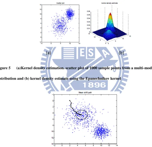
Figure 5 (a)Kernel density estimation. scatter plot of 1000 sample points from a multi-modal distribution and (b) kernel density estimate using the Epanechnikov kernel ... 10

Figure 6 The path defined by successive mean shift computations culminating to a local density maximum ... 10

Figure 7 KLT Algorithm flow chart ... 11

Figure 8 (a) 5*5 mask of Gaussian filter with σ=1 and (b) 2-D Gaussian distribution representation 12 Figure 9 (a) Input original frame (b) Gray level of Original frame (c) Gaussian Smooth of Original frame ... 13

Figure 10 (a) Input original frame (b) KLT corner detector of original frame ... 14

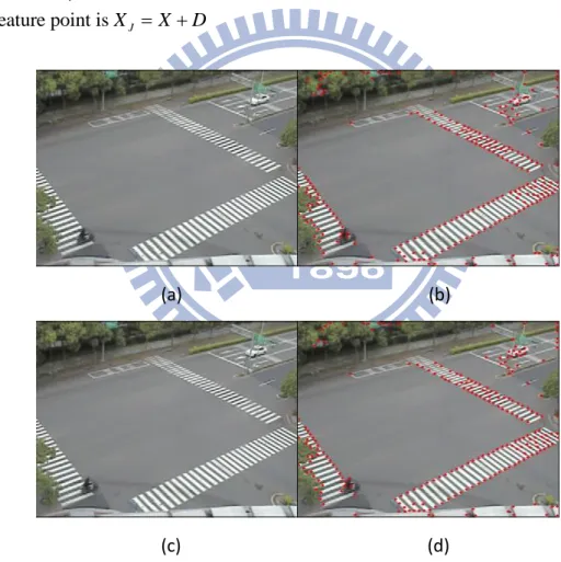
Figure 11 (a) Frame No.1 (b) Frame No.1 of KLT algorithm (c) Frame No.2 (d) Frame No.2 of KLT algorithm ... 15

Figure 12 The blue point is the guess feature points of frame no.2. The green line is the results of KLT algorithm ... 16

Figure 13 Object Grouping flow chart ... 18

Figure 14 Grouping condition flow chart ... 19

Figure 15 Video frame after KLT algorithm ... 20

Figure 16 (a) original frame1 (b) original frame2 (c) difference frame ... 20

Figure 17 (a) original frame (b) KLT frame (c) difference frame ... 21

Figure 18 (a) original frame (b) difference frame (c) distance frame ... 23

Figure 19 (a) Frame1 after KLT and difference (b) Frame2 after KLT and difference ... 24

Figure 20 Frame1 after OptKLT and difference... 25

ix

Figure 22 (a) original frame (b) distance frame (c) 4-direction gray level frame ... 27

Figure 23 (a) original frame (b) 4-direction gray level frame (c) clustering ... 27

Figure 24 Object identifier flow chart ... 28

Figure 25 The projection schematic diagram ... 30

Figure 26 The projection calculate ... 30

Figure 27 The solution of shape not the same ... 30

Figure 28 The solution of location not the same ... 30

Figure 29 The flow chart of on-lined update ... 31

Figure 30 The solution of occlusion ... 32

Figure 31 System flow chart ... 34

Figure 32 Experimental results of object detection ... 40

Figure 33 Experimental results of object tracking (a) frame1 (b) frame4 (c) frame7 (d) frame11 (e) frame15 (f) frame30. It is a normal case include car and monocycle ... 41

Figure 34 Experimental results of object tracking by KalmanFilte... 42

Figure 35 Experimental results of object tracking by Mean-shift ... 42

Figure 36 Experimental results of object tracking (a) frame380 (b) frame400 (c) frame450 (d) frame500 (e) frame550 (f) frame650. It is a special case about the white car that is green line, it is rotation. ... 43

Figure 37 Experimental results of object tracking (a) frame800 (b) frame820 (c) frame830 (d) frame840 (e) frame850 (f) frame900. It is special case about the two cars have the same velocity in frame800 to 820, but in frame840 they have different velocity in frame840 we can see the two cars locus that is yellow and green. ... 44

Figure 38 Experimental results of object tracking (a) frame2000 (b) frame2050 (c) frame2100 (d) frame2150 (e) frame2200 (f) frame225. It is a special case. That is many object enter the frame in the same time. At first they have the same velocity and they are very close. But in few frame, we can distinguish them. ... 45

Figure 39 Experimental results of object tracking (a) frame2000 (b) frame2050 (c) frame2100 (d) frame2150 (e) frame2200 (f) frame225. It is a special case. when occlusion occur between two cars. But we still can distinguish two cars. ... 46 Figure 40 Experimental results of object tracking (a) frame2000 (b) frame2050 (c) frame2100 (d)

frame2150 (e) frame2200 (f) frame225. It is a special case. That is a track and motorcycle. We just can find the track. Because they have the same velocity. But the track is not easy to

x

xi

List of Tables

Table 1 The based and common disadvantages of the Kalman filter ... 9

Table 2 The based and common disadvantages of the mean shift ... 10

Table 3 Grouping Condition Algorithm ... 18

Table 4 4-direction Gray Level Algorithm ... 24

Table 5 Object Identifier Algorithm ... 29

Table 6 Distance Algorithm ... 33

Table 7 Object Detection Algorithm ... 35

Table 8 Comparison Table ... 48

1

Chapter 1. Introduction

1.1. Motivation

In computer vision, many applications are built based on the tracking mechanism. For example, people counting, vehicle warning system, and security monitoring system as shown in Figure 1.[9][10] Tracking algorithm in the Human–Computer Interaction plays as communicator between human and computers. People can control the machines through the tracking algorithm. The computer can also accept and execute commands through the tracking mechanism. So how to design a good tracking method becomes an important research issues internationally.

Figure 1 The implement tracking in life

Ref: http://www.gps-navigations.net/wp-content/uploads/2010/09/Gps-Tracking-System.jpg Ref: Worldwide GPS Tracker with Two Way Calling, SMS Alerts, and More

2

Object tracking is a critical task in computer vision applications. The major challenges encountered are noise, occlusion, clutter and changes in the foreground object or in the background environment. Visual tracking in a cluttered environment remains one of the challenging problems in computer vision during the past few decades. Various applications such as surveillance, monitoring, video indexing and retrieval, require the ability to faithfully track objects in a complex scene involving appearance and scale change.

In computer vision, there are many tracking methods such as Kalman Filter, mean-shift, particle filter, and Kanade-Lucas-Tomasi (KLT) algorithms. But these methods are not perfect. They all have drawbacks and pose vulnerabilities. So many researchers still pay their attention on this problem, eager to provide revolutionary breakthroughs.

1.2. Objective

Most of the tracking algorithms can be broadly classified into following four categories. (1) Gradient-based methods which locate target objects in the subsequent frame by minimizing a cost function. (2) Feature-based approaches which use features extracted from image attributes such as intensity, color, edges and contours for tracking target objects. (3) Knowledge-based tracking algorithms which require a-priori knowledge of target objects such as shape, object skeleton, skin color models and silhouette. (4) Learning-based approaches which employ pattern recognition algorithms to learn the target objects in order to search them in an image sequence.

In the thesis, we’ve proposed a feature-based and learning-based efficient tracking mechanism that can function without using background, color, and special features. Because the mechanism does not refer special features of objects, it can track people, car, and motorcycle etc and use only gray image of the CCD camera with size 320x240.

3

In this thesis, we choose gradient-based and learning-based for our algorithm. We use the corner feature to track objects, because every object have corner features obviously. In advance, we cluster object with grouping and identifier and use learning machine to track object in the next frame.

1.3. Organization

This thesis is organized as follows. In the next chapter, we briefly review the related topic papers then describe methods and discuss the features which they adopted and presented. We also describe our algorithm in the language of Image processing. In chapter 3, the core techniques are described in detailincluding the inadequacy and disadvantage of the features. In chapter4, the main algorithm is presented. In chapter 5, we will show the experimental results and have a discussion on efficiency and reliability of the proposed algorithm. Finally, the conclusions of our algorithm and future works will be presented in chapter 6.

4

Chapter 2. Backgrounds

2.1. Overview

In recent years, many researchers have developed many techniques for tracking problem. The related topics to our research include “tracking object”, “KLT feature tracking”, “Kalman filter”, and “mean-shift” etc. In this chapter, these related works are classified by their different approaches. Furthermore, we will describe the problems which might happen in real situations. Section2.2 describes the "OpenCV" , the library we use in the program. In section 2.3, our research.

2.2. OpenCV

OpenCV[11] – "Open Source Computer Vision Library” is a library of programming functions focusing on real time computer vision. The library was originally written in C and this C interface makes OpenCV portable to some specific platforms such as digital signal processors.

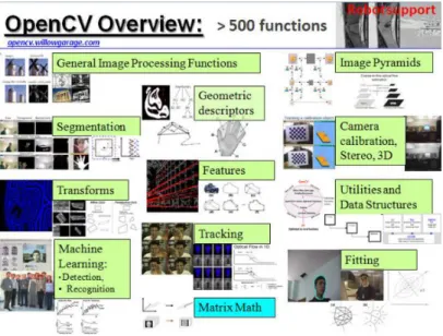
The application areas of OpenCV include: Motion tracking, Object Identification, and Motion understanding etc as shown in Figure 2. So we use the openCV source code to build our program.

5

Figure 2 OpenCV functions about computer vision

Ref: http://opencv.willowgarage.com/wiki/

2.3. Approaches Introduction

To distinguish the tracking for objects, many researchers have proposed diverse approaches which depend on different bases and using different features. We describe the most important bases which include “gradient-based”, “feature -based”, “knowledge -based”, and “learning-based” and introduce the most popular features briefly.

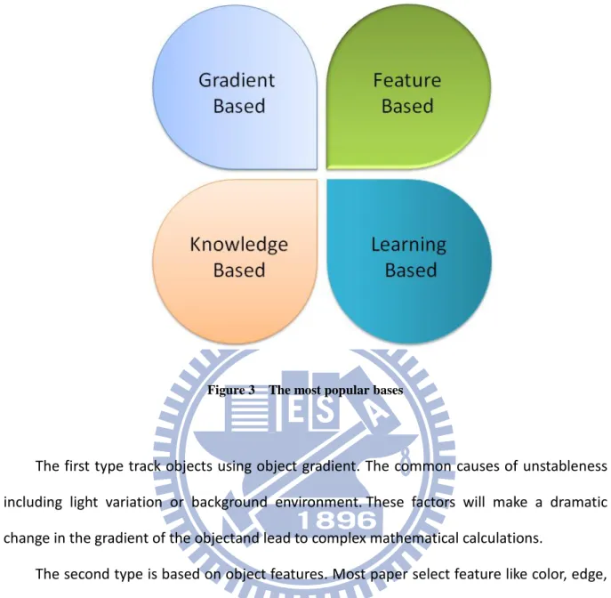
The most common features can be calssified into four typical types as seen in Figure 3. The mechanism may utilize one or integrate different bases to implement tracking objects.

6

Figure 3 The most popular bases

The first type track objects using object gradient. The common causes of unstableness including light variation or background environment.These factors will make a dramatic change in the gradient of the objectand lead to complex mathematical calculations.

The second type is based on object features. Most paper select feature like color, edge, and motion etc. If color feature is chosen, one cannot accurately capture the precise object color and compute current surrounding objects. When choosing edge feature, unbounded objects or unrecognizable boundaries may produce stronger edge intensity, and lead to false detection eventually. Most of the papers use the feature based methods, but it can only used to track a specific object. Here, we would like to implement an algorithm that can tracki any objects such as car, motorcycle, human, and any moving object.

The third type uses object knowledge to track. These methods detect specific characteristics of the target objects. For example, if we want to track human face, we will choose human skin, head, and facial organs. Using of the unique characteristics of the object

7 to tracking is knowledge based.

The forth type utilizes object learning to track. For example, SVM, Adaboost, and Bayesian. Those are using more samples to training for good tracking. So if one wants to conduct a good tracking, he should take abundant amount of samples from the tracking object.

2.4. Related Work

We will describe two popular methods: Kalman filter and Mean shift, and discuss there advantages and disadvantages. We also describe our algorithm based on the KLT algorithm.

2.4.1. Kalman filter

The purpose of Kalman filter[13] is to use measurements to observe over time, including noise and other inaccuracies, and produce values that approximate the true values of the measurements and their associated calculated values.

The Kalman filter is a recursive estimator. This means that only the estimated state from the previous time step and the current measurement are needed to compute the estimation for the current state. In contrast to batch estimation techniques, no history of observations and/or estimates are required. Afterwards, the notation Xˆn m| represents the

estimate of X at time n given observations up to, and including at time m.

8

 Xˆ_{k k|} , the a posteriori state estimate at time k given observations up to and including at time k;

 P_{k k|} , the a posteriori error covariance matrix.

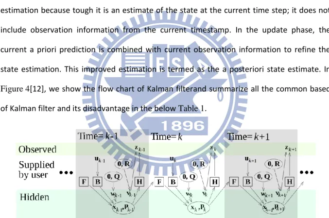
The Kalman filter can be written as a single equation; however it is most oftenly conceptualized as two distinct phases: "Predict" and "Update". The predict phase uses the state estimated from the previous time step to produce an estimation of the state at the current time step. This predicted state estimation is also known as the a priori state estimation because tough it is an estimate of the state at the current time step; it does not include observation information from the current timestamp. In the update phase, the current a priori prediction is combined with current observation information to refine the state estimation. This improved estimation is termed as the a posteriori state estimate. In Figure 4[12], we show the flow chart of Kalman filterand summarize all the common based of Kalman filter and its disadvantage in the below Table 1.

Figure 4 Model of Kalman filter

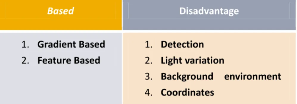
9 Based Disadvantage 1. Gradient Based 2. Feature Based 1. Detection 2. Light variation 3. Background environment 4. Coordinates

Table 1 The based and common disadvantages of the Kalman filter

2.4.2. Mean shift

The mean shift[2] estimation of the gradient of a density function and the associated iterative procedure of mode seeking has been developed by Fukunaga and Hostetler recently; however, the nice properties of data compaction and dimensionality reduction of the mean shift have been exploited in low level computer vision tasks. A nonparametric estimator of density gradient, the mean shift, is employed in the joint, spatial-range domain of gray level and color images for discontinuity preserving filtering and image segmentation.

The main idea behind the mean shift procedure is to treat the points in the d-dimensional feature space as an empirical probability density function, where the densest regions in the feature space correspond to the local maxima or modes of the underlying distribution. Figure 5[2] is the Mean-shift kernel model, and Figure 6[2] shows the convergence.

In section 2.4.1 and 2.4.2, we describe the most popular tracking methods, Kalman filter and Mean-shift. Many people use these functions to improve better methods for tracking. Kalman filter needs color information and background subtraction. Mean-shift also needs color information and image segmentation. So we choose KLT algorithm as our algorithm basis. In section2.5, we will describe KLT algorithm advantage and it execution steps. We summarize all the common type of bases of mean shift and its disadvantage in the below Table 2.

10 Based Disadvantage 1. Gradient Based 2. Feature Based 1. Detection 2. Color information 3. Background environment

Table 2 The based and common disadvantages of the mean shift

(a) (b)

Figure 5 (a)Kernel density estimation. scatter plot of 1000 sample points from a multi-modal

distribution and (b) kernel density estimate using the Epanechnikov kernel

Figure 6 The path defined by successive mean shift computations culminating to a local density

maximum

Ref: Konstantinos G. Derpanis, Mean Shift: Construction and Convergence Proof, November 26, 2006

11

2.5. KLT algorithm

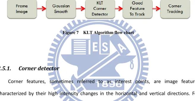
KLT[7] is a gradient based tracking providing functions of a feature tracker for the computer vision community programmed in C.. Figure 7 is the KLT future tracking flow chart. KLT has been designed for easy and convenience. It barely takes minutes learning how to select, track features, store and use the results. For those who wish to maximize the performance, luckily, the program also poses the flexibility for we to tweak nearly every parameter that governs the computation, and it includes several methods to improve speed.

Figure 7 KLT Algorithm flow chart

2.5.1. Corner detector

Corner features, sometimes referred to as interest points, are image features characterized by their high intensity changes in the horizontal and vertical directions. For instance, if a square object is present in the image then its four corners are prominent interest points. Corners impose more constraint on the motion parameters than edges; therefore the full optic-flow field is recoverable at corner locations. Corners appear more frequently therefore can provide more abundant information than straight edges in the natural world, making them ideal features to track in an indoor and outdoor environment.

Corner detection[1] has four methods: Kitchen-Rosenfeld[20], the Harris[21], the KLT[23] and the Smith[22] corner detectors. The Kitchen-Rosenfeld method uses first and second order derivatives in calculating the orneriness value, while Harris method uses only first order derivatives. The Smith method uses a geometrical criterion in calculating the corniness value, while KLT detector uses information from an inter-frame point displacement technique

12 to declare corners.

The Kitchen-Rosenfeld method does not use a built-in smoothing function and also has second order derivatives, and as a result its’ performance is poorer than the Harris method. The corners extracted by the Kitchen-Rosenfeld and the Smith detectors are less desirable for point feature tracking in long image sequences. The overall empirical results revealed that the KLT and Harris detectors provided the best quality corners. We choose the KLT corner detector as our system of corner detector.

2.5.2. KLT Corner detector

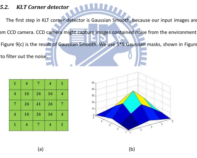
The first step in KLT corner detector is Gaussian Smooth, because our input images are from CCD camera. CCD camera might capture images contained noise from the environment. In Figure 9(c) is the result of Gaussian Smooth. We use 5*5 Gaussian masks, shown in Figure 8, to filter out the noise.

(a) (b)

13

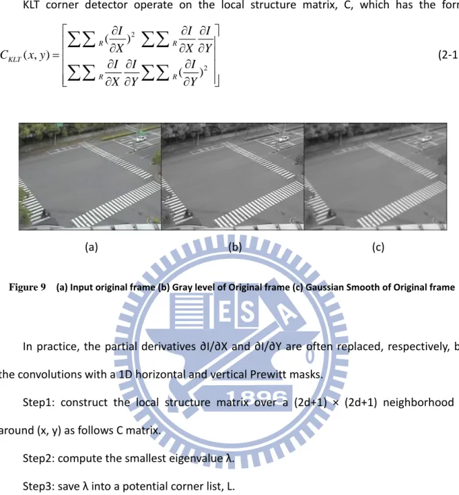
KLT corner detector operate on the local structure matrix, C, which has the form

2 2 ( ) ( , ) ( ) R R KLT R R I I I X X Y C x y I I I X Y Y       _{  }           _{  }   









(2-1) (a) (b) (c)

Figure 9 (a) Input original frame (b) Gray level of Original frame (c) Gaussian Smooth of Original frame

In practice, the partial derivatives ∂I/∂X and ∂I/∂Y are often replaced, respectively, by the convolutions with a 1D horizontal and vertical Prewitt masks.

Step1: construct the local structure matrix over a (2d+1) × (2d+1) neighborhood R around (x, y) as follows C matrix.

Step2: compute the smallest eigenvalue λ. Step3: save λ into a potential corner list, L. Step4: sort L in decreasing order of λ.

Step5: Scan the sorted list from top to bottom and select points in the list in sequence. Points that fall inside the neighborhood R of any selected points are removed.

We use the openCV library about KLT corner detector is "cvGoodFeaturesToTrack." In Figure 10, we show the original frame, and use "cvGoodFeaturesToTrack" function to show the KLT frame. In "cvGoodFeaturesToTrack" function every frame that we choose the 500 corners. In KLT frame the red point is the corner location that the results of function.

14

(a) (b)

Figure 10 (a)Input original frame (b) KLT corner detector of original frame

2.5.3. KLT Corner tracking

Pyramidal Implementation of the Lucas Kanade Feature Tracker is the most important implement of KLT corner tracking. The two key components to any feature tracker are accuracy and robustness. The accuracy component relates to the local sub-pixel accuracy attached to tracking. The robustness component relates to sensitivity of tracking with respect to changes of lighting, size of image motion, In particular, in order to handle large motions, it is intrusively preferable to pick a large integration window. In provide to provide a solution to that problem, we propose a pyramidal implementation of the classical Lucas-Kanade algorithm. An iterative implementation of the Lucas-Kanade optical flow computation provides sufficient local tracking accuracy.

We introduce the following steps of KLT corner tracking. Step (1) KLT corner detector (feature points).

Step (2) Using feature points to track. Step (3) Solving the linear equation.

Step (4) Determine whether the convergence.

15

equation (2-2). In step (4), Iteration D (t+1) = D (t) + ΔD. If iterations<TH or ΔD<TH, then Iteration over. If not, repeat (2) ~ (4) until ε converge.

(1) (2) (a) (b) (c) (d)

Figure 11 (a) Frame No.1 (b) Frame No.1 of KLT algorithm (c) Frame No.2 (d) Frame No.2 of KLT

algorithm

2

= [ ( ) ( )] ( )

: Image that feature points have been found : Image that feature points havn't been found

[ , ] :any feature point on Imag I

[ , ] feature point displacement

: estimat w T x y J X D I X X dX I J X x y D d d       



: ion error -1 Solving [ , ]

Image J feature point is

T x y J D Z e D d d X X D    

16

We show the two consecutive frames of input video, shown in Figure 11 (b) (d), and use these frames to run the KLT algorithm function. The KLT algorithm result as shown in Figure 12. The green line is the corners guess way.

Figure 12 The blue point is the guess feature points of frame no.2. The green line is the results of KLT

algorithm

2.5.4. Discussion

In KLT algorithm, it just uses gray level, and corner feature is easier than another algorithm. But in Figure 12, KLT algorithm just can implement corner features tracking. It can’t know that the corner features is on the which object. So how to use KLT algorithm to implement object tracking is the key point in the thesis.

17

Chapter 3. Proposed Techniques

3.1. Objective

In last chapter, we can find the related work to improve tracking have some restriction and shortcoming. We approach using two different based including gradients based and learning based. Therefore, we proposed the three core techniques in this chapter in order to promote the precision and plasticity of the tracking system.

The three main core techniques are: 1. Object grouping method, 2. Object Identifier and 3. On-lined Update. The first technique uses a new tool to group moving objects in video frame. The second technique uses a new tool to identify objects to tracking. And the third technique On-lined tools to learning. We introduce the details of the core techniques and explain how they can solve the inadequacy of the features.

3.2. Object Grouping

3.2.1. Objective

In KLT algorithm, it just point to point tracking. We know the point location at next frame. But we don’t know the object location. For many tracking method, that can use some methods, like connected component to find the moving objects. So how to group the moving objects is a problem in KLT algorithm. In this section, we describe the methods to group the object. The object grouping includes “Grouping condition”, and “4-direction Gray Level”. In Figure 13, we show the flow chart for object grouping. The method of Object Grouping is shown as Table 3.

18

Algorithm

G

ROUPING

C

ONDITION

Input: KLT Feature Point [i], for i = 0, 1, 2, 3,..., FeatureNo Output: An object Number[k], for k = 0, 1, 2, 3,...

If KLT Feature Point Number > 0 For i=0 to FeatureNo

If Difference (KLT Feature Point [i] ) > TH

For j=0 to FeatureNo

If Distance (KLT Feature Point [i], KLT Feature Point [j] ) < TH Number[j] Number[i] End If End for End if End for End if

Table 3 Grouping Condition Algorithm

19

3.2.2. Grouping Condition

The grouping condition is the preprocessing to object grouping. We can use grouping condition to find the moving objects. In Figure 14, that shows the flow chart of grouping condition.

Figure 14 Grouping condition flow chart

We propose two methods to grouping objects. We use the difference of video frame to find the moving objects. And we use the distance to find the feature points on the same objects.

I. Difference

After KLT algorithm, we can get the video frame that have the feature points in Figure 15. In Figure 15, it show the all feature points on video frame. But it has much feature points that we don’t interest. We use KLT algorithm to get feature points, but we just want to get the feature points that is on the moving objects.

After KLT algorithm, we get the less than five hundred feature points. We should get more feature points by KLT algorithm. Because it have stronger information in environment that is on the intersection index, zebra crossing, and some noise. If we want to get more feature points, just change threshold.

20

Figure 15 Video frame after KLT algorithm

After KLT algorithm, we get the less than five hundred feature points. We should get more feature points by KLT algorithm. Because it have stronger information in environment that is on the intersection index, zebra crossing, and some noise. If we want to get more feature points, just change threshold.

In Figure 16, we show the two consecutive frames difference images. By difference, it can find the move objects in original frame.

(a) (b) (c)

Figure 16 (a) original frame1 (b) original frame2 (c) difference frame

We can use the same coordinate to subtraction with the information of gray level of two consecutive frames. We call the difference (I, J) of each frame. If the difference (I, J) is

21

bigger than TH = 30, as shown in (3-1), that is the moving object.

255, ( ( ) ( )) ( , )= 0, ( ) : gray level of a difference if G I G J TH difference I J otherwise G a      (3-1)

After difference, we can find the moving object. We can use this result to cut the feature points. If the feature points are on the moving objects, we choose the feature points. Otherwise we delete it. Using the difference result the feature points that is we interested as shown in Figure 17.

(a) (b) (c)

Figure 17 (a) original frame (b) KLT frame (c) difference frame

In Figure 17(b) is the KLT algorithm results that we named KLT frame. After difference we get the result in Figure 17(c) that we named difference frame. In difference frame we can find the feature points is less than KLT frame and all the feature points are on the moving objects. In this step, we significantly reduced the number of feature points. And it does not affect our algorithm.

22

II. Distance

In difference frame, we can find the feature points which are on the moving objects. But we can not know the feature points that are on the same object. We want to group the feature points on the same moving objects. KLT algorithm just feature points to feature points tracking. But in this thesis we want to improve the moving objects tracking based on KLT algorithm. We find the method to solve this problem named distance.

We use the concept that the feature points are close on same moving objects. Through the methods, it can group more objects except the closing objects or occlusion objects. We find the distance of each feature points in (3-2). Through the function, it can find the distance in the video frame of each feature points. Using this results, we define the TH = 10.

(3-2)

Using the above two formulas, we can simply to find the group of feature points. In Figure 18, we show the result by distance named distance frame. If the feature points are on the same object, it has the same color. We defined the four colors to show the group. In KLT algorithm, every feature points have its own number. In distance, if two feature points is group, that the one feature point number is not to change another feature point number is change to its group feature point. After distance, if it have three moving objects in the video frame, and all the feature points into three group that have own number.

tan tan ( ) ( ) , D( ) ( , ) , , D( ) ( , ) , i j i j i i i x x dis ce x x x xi dis ce x x D s s t t if I I TH D I I otherwise if I J TH D I J otherwise                 2 2 1 2 1 2 1 0 1 0

23

(a) (b) (c)

Figure 18 (a) original frame (b) difference frame (c) distance frame

It shows all the feature points in difference, but we can't know the group of feature points. After difference, we can find the same groups of feature points have the same color as shown in Figure 18(c).

3.2.3. 4-direction Gray Level

After difference, we know the groups of feature points. Next step we want to show the full of object in the video frame. We define the algorithm named 4- direction gray level as shown in Table 4. The algorithm is based on fuzzy concept, and use relatively small number of calculations to draw the object shape.

The feature points are on the objects after difference. Using the two consecutive frames, we can find the moving objects. In Figure 19, we show the two consecutive frames after KLT algorithm and difference.

24

Algorithm

4-

DIRECTION

G

RAY

L

EVEL

Input: KLT Now Feature Point [i], for i = 0, 1, 2, 3,..., FeatureNo

KLT Next Feature Point [i], for i = 0, 1, 2, 3,..., FeatureNo

Output: An object Number[k], for k = 0, 1, 2, 3,... If KLT Now Feature Point Number > 0

For i=0 to FeatureNo

If Difference (KLT Feature Point [i] ) > TH

If SimilarUP (KLT Now Feature Point [i], KLT Next Feature Point [j] ) >90% pixel(x,y) object Number[k]

If SimilarPixelNumber > (Rows PixelNumber)/2 go to next row End If End If End If End For End If

Table 4 4-direction Gray Level Algorithm

(a) (b)

25

Figure 20 Frame1 after OptKLT and difference

In the two consecutive frames, the feature points not always the same. The same object in different frame, it has different number feature points as shown in Figure 19. Because the KLT feature points are not stable, we can't use it to check the objects. We use the same frame to improve opencv KLT tracking, the results as shown in Figure 20. The green points are the feature point of this frame. The red points are the guess feature points in the next frame. So we use the results to compare the gray level.

In now frame, choose the feature point A, and feature point A' in next frame. Using two vertical lines through the feature point as shown in Figure 21. Using two lines we can get the four direction of feature point. It have up, down, left and right four directions.

After direction, we have A and A' feature points. First, we through the up direction to compare. We can get the A(x-1,y) and A'(x-1,y),and they have own gray level named GrayA and GrayA'.. And the feature point named Similar(A,A'), as shown in (3-3). The TH means GrayA and GrayA' gray level similar more than 90%.

26

Figure 21 Feature point 4-direction

(3-3)

(3-4)

Through the two vertical lines, it shows the four directions have many rows. In Figure 21, it shows the first row have one pixels, second row have three pixels as show in (3-4). In the now frame up direction first row named RowA and RowA’ is the next frame. If RowA and RowA’ are similar then we go to next row. We get the total pixel number in the row, if more than half pixel number is similar. Then we define RowA and RowA’ are similar.

After 4-direction gray level, we can draw the object more complete as shown in Figure 22. Using 4-direction gray level we can avoid the object shape is not round. Even the object is bizarre shape, we can use this method to solve. In Figure 22(c), we can find the object easily. From feature points to generate objects, through our algorithm Object Grouping. And we can

G(I )-G(I ) 1, 0.1 (I ) G(I ) 0, i j i i x x x x if PixelSimilar otherwise        ( ) 1, 0.5 0, i x i PixelSimilar I if RowSimilar PixelNumber otherwise   _    



27

use results to clustering the object as shown in Figure 23.

(a) (b) (c)

Figure 22 (a) original frame (b) distance frame (c) 4-direction gray level frame

Figure 23 (a) original frame (b) 4-direction gray level frame (c) clustering

3.3. Object Identifier

3.3.1. Objective

After object grouping, we can find the object in the video frame. In next frame we should find the same object give the same number that is tracking main points. In many tracking methods, they use features to compare objects. In our Algorithm, we just have gray level and KLT feature points. So we use the KLT feature points to compare to find the same object.

28

3.3.2. Object Identifier

By 4-direction gray level, we get the object location. And we get the feature points guess displacement in next frame by KLT tracking algorithm. So we have each feature points guess displacement, and its region through 4-direction gray level. We show the algorithm of object identifier in Table 5 and flow chart in Figure 24.

Figure 24 Object identifier flow chart

We use the guess displacement and now frame location to estimate the object location in next frame. It is projection concept, it can help me to solve the object doesn't have KLT feature points in next frame. KLT feature points are not stable. If object occur has covered by other car or the object too small that it can’t find its feature points. If we detect the object in now frame, we can find it in next frame. We find the object region in next frame; we have the region to do object grouping in next frame. If the object lost in next frame, we can guess it has been covered. We also guess its location in next two frames. The projection algorithm is shown in Figure 25 and Figure 26.

29

Algorithm

O

BJECT

I

DENTIFIER

Input: KLT Feature Point Region [i], for i = 0, 1, 2, 3,..., FeatureNo

KLT Feature Point Guess Displacement [i], for i = 0, 1, 2, 3,..., FeatureNo

Output: New KLT Feature Point Region [i], for i = 0, 1, 2, 3,... If KLT Now Feature Point Region[i] > 0

For i=0 to FeatureNo

If Difference (KLT Feature Point Region [i] ) > TH New KLT Feature Point Region[i]

KLT Feature Point Region [i] + KLT Feature Point Guess Displacement [i]

End If End For End If

Table 5 Object Identifier Algorithm

We get the guess location in next frame. In next frame, we can also use KLT algorithm and Object Grouping to get the real location. If real location and guess location are difference, it wills occlusion. The problems have two cases, one is the location is the same but the object shape is more difference. The solution of this case, we believe that is occlusion. So we use guess location as correct solution. The solution is shown in Figure 27. Another case is the shape is the same but the location is not. The solution of this case, we guess it suddenly accelerates. We use guess location and real location average as correct location. The solution is shown in Figure 28.

30

Figure 25 The projection schematic diagram

Figure 26 The projection calculate

Figure 27 The solution of shape not the same

Figure 28 The solution of location not the same

Original Object Guess Displacement Original Object Projection New Object Guess Location Xi Yi moveXi moveYi NewXi NewYi Real Location Guess Location Real Location Correct Location Guess Location Real Location Guess Location Real Location Guess Location Real Location Correct Location

31

3.3.3. On-lined Update

In 3.3.2, we can find the problem that the object occur occlusion. If object occur occlusion, its KLT feature point will reduce in next frame. Because the occlusion part of the object can’t not use KLT algorithm. We define the on-lined update to guess the KLT feature point's location if it doesn’t have KLT feature points in around. The algorithm flow chart as shown in Figure 29.

Figure 29 The flow chart of on-lined update

If the guesses feature points and real feature point's location are difference. We will check the real feature points around, if it doesn’t have another feature points. The guess feature points will inherit as correct feature points. If real object occur occlusion, the part of occlusion KLT feature points haven't detect. So the guess KLT feature points on the part of occlusion will inherit as correct feature points. We will guess KLT feature points the same part of continues three frames. If more than three frames, the part of the object always can’t detect KLT feature points. We will give up inheriting feature points. We guess the object occur deformation.

32

velocity and occur occlusion. At the beginning, we can’t distinguish which object just define it is big object. After few frames, if they have different velocity their location will separate slowly. After Object Grouping, we will do distance function continued. The distance function is not the same with 3.3.1. We show the distance algorithm in Table 6.

Through this algorithm, we can distinguish the object that is occlusion before. The results as shown in Figure 30. In Figure 30 (a), we can find the two yellow cards in frame. After few frames the car is not occlusion. We can distinguish it is not the same right now. We show the two different cars in Figure 30 (b).

(a) (b)

33

Algorithm

D

ISTANCE

Input: KLT Feature Point [i], for i = 0, 1, 2, 3,..., FeatureNo

Object Number[i], for i = 0, 1, 2, 3,..., FeatureNo

Output: Object Number [i], for i = 0, 1, 2, 3,... If KLT Now Feature Point Region[i] > 0

For i=0 to FeatureNo

For j=0 to FeatureNo

If Object Number[i] = Object Number[j]

If distance(KLT Feature Point [i] - KLT Feature Point [j]) > TH Object Number[j] Object Number[i]+1

End If End If End For

End For End If

34

Chapter 4. System Architecture

4.1. Overview

After completely introducing three main techniques of the system, we will dissect main algorithm of the system in this chapter. Our system can be categorized into two main parts: 1. Object Detection and 2. Object Tracking. The comprehensive algorithm flow chart is shown in the Figure 31. System starts with KLT algorithm, then it enter the gray box of the flow chart. The green block is about object detection which is described in the Section 4.2. After completion in Object locating, the process subsequently apply Object tracking procedure as shown in blue block of the flow chart and we discuss it in Section 4.3.

35

4.2. Object Detection

Our Object detection has KLT algorithm and Object Grouping. Evert frame enter in our algorithm should be through KLT algorithm. After KLT algorithm, every frame gets the KLT feature points in video frame named KLT frame. If video frame is zero then KLT frame enter Object Grouping. Object Grouping has grouping condition and 4-direction. We can get the KLT feature points in moving object by grouping condition. And the moving object has been detected by 4-direction gray level.

Through our object detection, we can find the every moving object. In tracking methods, we must find the moving objects first. After detection compare the moving objects to tracking. In Table 7, we show the object detection algorithm.

Algorithm

O

BJECT

D

ETECTION

Input: Video Frame[i], for i = 0, 1, 2, 3,..., FrameNo Output: Object Number [i], for i = 0, 1, 2, 3,...

If Video Frame [i] = 0

KLT Frame KLT (Video Frame)

Object Feature Points Frame Grouping Condition (KLT Frame)

Object Number [i] 4-direction Gray Level (Object Feature Points Frame) Save Object number[i] and Object location[i]

End If

Table 7 Object Detection Algorithm

After Object Detection, we get the moving object and its own number. We will remember the object number and location and write it in the memory. Then the on-lined update machine will to load the memory to use it.

36

4.3. Object Tracking

If video frame number is zero then after object detection, we will find the moving object. And video frame number will add one to do object tracking. Because every frame enter will do KLT algorithm. If video frame is not zero, we will use the KLT frame to compare the before frame. In Object Identifier, we find the old objects in new frame. If we find the object is in the two consecutive frames, defined the object own number. If we can find the object in previous frame, we define the object is new. For new object, we will do object detection again. The Object Tracking algorithm is shown in Table 8.

Algorithm

O

BJECT

T

RACKING

Input: Video Frame[i], for i = 0, 1, 2, 3,..., FrameNo

Object Number[i], for i = 0, 1, 2, 3,...

Output: Object Number[i], for i = 0, 1, 2, 3,... If Video Frame [i] > 0

On-lined Update Object Grouping (Previous frame) KLT Frame KLT (Video Frame)

Object Number[i] Object Identifier (KLT frame) If New KLT feature points

New object Object detection (New KLT feature points)

On-lined Update New object

Else

Old object Object Grouping (KLT feature points) On-lined Update Old object

End If

End If

Table 8 Object Tracking Algorithm

We use the KLT feature points to compare the guess KLT feature points. If we defined the KLT feature points is the same, then it using the old number. And guess object location

37

compare the real object to get the correct object. The correct objects also use the old number. If the KLT feature points is new, we should do object detection and object grouping define the location. All the information will send to the On-lined Update machine to modify object location in next frame.

38

Chapter 5.

Experimental Results

In this chapter, we will show our results of object detection and object tracking in Section 5.1 and Section 5.2. We implemented out algorithm on the platform of PC with Intel core i5-460 2.53GHz and 4GB RAM. The software we used is Borland C++ Builder on Windows 7 OS and use OpenCV Library. All of the testing videos are uncompressed AVI standard files. The resolution of video frame is 320240. And frame per second is 28.

5.1.

Experimental Results of Object Detection

In the following, we show our experimental results of object detection. At first, we present the environment of the original frame as the left image of the raw in Figure 32, and show the object detection algorithm as the right image of the raw in Figure 32. In Figure 32, they include many type of object.

(a) (b) Figure continues

39

(c) (d)

(e) (f)

(g) (h) Figure continues

40

(i) (j)

(k) (l)

Figure 32 Experimental results of object detection

5.2.

Experimental Results of Moving Object Positioning

Here, we demonstrate some object tracking examples. At first, we present the environment of the original frame as the up image of the raw in Figure 33 to Figure 40, and show the object tracking algorithm as the down image of the raw in Figure 33 to Figure 40. It has normal case and some special case. In Figure 34 and Figure 35 is the same video with Figure 36. But Figure 34 is used Kalman Filter and Figure 35 is used mean-shft. In Table 8, we

41

show the comparison algorithm between reference and ours. In Table 9, we show the comparison algorithm between Kalman filter and ours.

(a) (b) (c)

(d) (e) (f)

Figure 33 Experimental results of object tracking (a) frame1 (b) frame4 (c) frame7 (d) frame11 (e)

42

Figure 34 Experimental results of object tracking by KalmanFilte

43

(a) (b) (c)

(d) (e) (f)

Figure 36 Experimental results of object tracking (a) frame380 (b) frame400 (c) frame450 (d) frame500

44

(a) (b) (c)

(d) (e) (f)

Figure 37 Experimental results of object tracking (a) frame800 (b) frame820 (c) frame830 (d) frame840

(e) frame850 (f) frame900. It is special case about the two cars have the same velocity in frame800 to 820,

but in frame840 they have different velocity in frame840 we can see the two cars locus that is yellow and

45

(a) (b) (c)

(d) (e) (f)

Figure 38 Experimental results of object tracking (a) frame2000 (b) frame2050 (c) frame2100 (d)

frame2150 (e) frame2200 (f) frame225. It is a special case. That is many object enter the frame in the same

time. At first they have the same velocity and they are very close. But in few frame, we can distinguish

46

(a) (b) (c)

(d) (e) (f)

Figure 39 Experimental results of object tracking (a) frame2000 (b) frame2050 (c) frame2100 (d)

frame2150 (e) frame2200 (f) frame225. It is a special case. when occlusion occur between two cars. But we

47

(a) (b) (c)

(d) (e) (f)

Figure 40 Experimental results of object tracking (a) frame2000 (b) frame2050 (c) frame2100 (d)

frame2150 (e) frame2200 (f) frame225. It is a special case. That is a track and motorcycle. We just can

find the track. Because they have the same velocity. But the track is not easy to distinguish in other

48

Mean-shift Kalman filter KLT UVLAB

Based Gradient + Feature Gradient + Feature Gradient Gradient + Learning

Color Yes No No No

Create background No Yes No No

Object boundary No No No Yes

Object tracking Yes Yes No Yes

Occlusion sometimes No No Objects have

been separated

FPS Real time Real time Real time 28

Table 8 Comparison Table

Sample1 Sample2

Object numver Kalman fikter UVLAB Kalman fikter UVLAB

Tracking object 97 97 29 29

Tracking rate 64 85 18 27

False alarm 66% 87% 62% 93%

Object tracking 0 0 20 0

Kalman filter will use 400 frames to crate background

49

Chapter 6. Conclusion

6.1. Achievements

We present a new method of efficient object tracking real-time performance. At first, we use the KLT algorithm to find the KLT feature points, and then perform the object detection algorithm include object grouping. In the algorithm, we utilize the difference, distance, and 4-direction gray level in the detection object. In our tracking, we don’t need to establish background. So we are not afraid to environment change. And avoid waste time to establish background.

In this paper, we proposed a new method which combines gradient based and learning based. Therefore, we enhance the preciseness of the system. In addition, our algorithm has modified most disadvantages of the feature based. Firstly, we proposed the KLT algorithm. We just search the corner of the objects. So it can avoid the special feature just on special objects. Secondly, we solve the some problem of most tracking methods disadvantages. And our algorithm time complexity is low latency.

Experiments were conducted on different scenes which including the different type of objects and special case. The system succeeds in detecting and tracking the normal case. Our system can also accommodate the big car, occlusion, and rotation etc. Through the experiment, we realize the overall excursion time is very swift. In the future, we believe that when the system ports to the platform; it can achieve real-time performance as well.

50

6.2. Future Works

To further improve the performance and the robustness of our algorithm, some enhancements or trials can be made in the future. Firstly, if the object it too small the KLT feature points can’t be searched. Therefore, we can choose another feature to help the case. And we use the difference to delete KLT feature points. If object stay in the same place, we can’t find it. So how to save the KLT feature points and hedge the object is leave or stay that is a good problem to solve.

After accomplishing the overall functions mentioned above, the system will very applicable and we will transplant from PC based to DSP platform for more commercial certification and appealing.

51

References

[1] P. Tissainayagam, D. Suter, Assessing the performance of corner detectors for point feature tracking applications, Image and Vision Computing 22 (2004) 663–679

[2] Konstantinos G. Derpanis, Mean Shift: Construction and Convergence Proof, November 26, 2006

[3] Valtteri Takala and Matti Pietik¨ainen, Multi-Object Tracking Using Color, Texture and Motion, 2007.

[4] Helmut Grabner, Michael Grabner, Horst Bischof, Real-Time Tracking via On-line Boosting

[5] Jifeng Ning, Lei Zhang, David Zhang, Chengke Wu, Robust Object Tracking Using Joint Color-Texture Histogram, International Journal of Pattern Recognition and Artificial Intelligence Vol. 23, No. 7 (2009) 1245ttern

[6] R. Venkatesh Babu, Patrick Peern , Patrick Bouthemy, Robust tracking with motion estimation and local Kernel-based color modeling, Image and Vision Computing 25 (2007) 1205local

[7] Jean-Yves Bouguet, Pyramidal Implementation of the Lucas Kanade Feature Tracker Description of the algorithm

[8] Corner Detection and Tracking, Computer Vision CITS4240

[9] http://www.gps-navigations.net/wp-content/uploads/2010/09/Gps-Tracking-System.jpg [10] Worldwide GPS Tracker with Two Way Calling, SMS Alerts, and More

[11] http://www.opencv.org.cn/

[12] http://en.wikipedia.org/wiki/Kalman_filter

[13] Greg Welch , Gary Bishop , An Introduction to the Kalman Filter, UNC-Chapel Hill, TR 95-041, July 24, 2006

52

[14] Elaine Pettit and Dr. Kathleen M. Swigger, An Analysis of Genetic-based Pattern Tracking and Cognitive-based Component Tracking Models of Adaptation, AAAI-83 Proceedings

[15] Zhixu Zhao, Shiqi Yu, Xinyu Wu, Congling Wang, Yangsheng Xu, A Multi-target Tracking Algorithm using Texture for Real-time Surveillance, 2008 IEEE International Conference on Robotics and Biomimetics Bangkok, Thailand, February 21 - 26, 2009.

[16] Xian WU, Lihong LI, Jianhuang LAI, Jian HUANG, A Framework of Face Tracking with Classification using CAMShift-C and LBP, 2009 Fifth International Conference on Image and Graphics

[17] Carlo Tomasi, Takeo Kanade, Detection and Tracking of Point Features, Technical Report CMU-CS-91-132 April 1991

[18] Tracking features using the KLT algorithm, VGIS 821 April 21, 2009

[19] KLT: An Implementation of the Kanade-Lucas-Tomasi Feature Tracker,

http://www.ces.clemson.edu/~stb/klt/

[20] L. Kitchen, A. Rosenfeld, Gray level corner detection, Pattern Recognition Letters (1982) 95–102

[21] C.G. Harris, M.J. Stephens, Combined corner and edge detector, In Proceedings of the Fourth Alvey Vision Conference, Manchester 147–151, 1988

[22] S.M. Smith, J.M. Brady, SUSAN—a new approach to low level image processing, International Journal of Computer Vision 23 (1) 45–78, 1997

[23] C. Tomasi, T. Kanade, Detection and Tracking of Point Features, Carnegie Mellon University, Tech. Report CMU-CS-91-132, April, 1991.