ADAPTIVE NONLINEAR DECISION-FEEDBACK EQUALIZATION WITH CHANNEL ESTIMATION AND TIMING RECOVERY IN DIGITAL MAGNETIC RECORDING-SYSTEMS

196 IEEE TRANSACTIONS ON CIRCUITS AND SYSTEMS-11: ANALOG AND DIGITAL SIGNAL PROCESSING, VOL. 42, NO. 3, MARCH 1995

Adaptive Nonlinear Decision Feedback Equalization

with Channel Estimation and Timing Recovery

in Digital Magnetic Recording Systems

Jui-Yuan Lin

and

Che-Ho

Wei, Senior Member, IEEE

Abstract-In high density digital magnetic recording systems, the nonlinear effects in the write process appear in the readback waveform as shifts in the peak positions and changes in the ampli- tude. The pulse shift causes a nonlinear intersymbol interference (ISI) on the readback signal. In this paper, a Volterra-DFE, in which a Volterra filter is used in the feedback section of decision feedback structure, is proposed to equalize the nonlinear ISI. By theoretical analysis, the minimum mean squared error (MSE) of the Volterra-DFE is found to be a function of sampling phase. This will affect the output signal-to-noise ratio (SNR) of the playback system. A baud-rate timing recovery system in conjunction with channel estimator is used to operate the sampling clock on the optimum phase. By computer simulation, Volterra-DFE is found to outperform conventional DFE in both output SNR and BER in a high density magnetic recording system.

I. INTRODUCTION

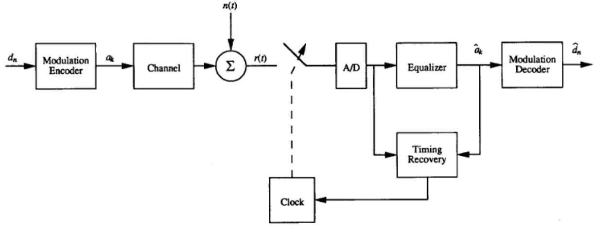
N the digital magnetic recording system, as shown in Fig. 1,

I

the binary data sequence d, at a data rate l/Ts is encoded

to a binary sequence U k E {-1, +1} at the rate 1/T by the modulation encoder, and then written into the recording media. For a linear saturation recording system, the playback signal from the read head is given by [l]

T ( t ) = ; ( U k - a k - l ) s ( t - kT)

+

n(t) (1)

k

where s ( t ) is the isolated transition (step) response of the

recording channel, and n(t) is an additive white Gaussian

noise. In general, the isolated transition response can be modelled by a Lorentzian function, given by

s ( t ) = 1

1

+

( 2 t / p ~ 5 0 ) ~

where pw50 is the width of the transition pulse at 50% of its

peak value.

When the spacing of adjacent transition pulses is large, the readback signal is often modelled by a linear superposition of isolated transitions, as described in (1). Due the nonideal characteristic of the transition pulse in the recording channel,

Manuscript received December 13, 1993; revised June 14, 1994. This paper was recommended by Associate Editor L. R. Carley. This paper was presented in part at the IEEE Symposium on Circuits and Systems, London, England, May 1994.

The authors are with the Institute of Electronics and Center for Telecom- munications Research, National Chiao Tung University, Hsin Chu, Taiwan, R.O.C.

IEEE Log Number 9407655.

intersymbol interference (ISI) is often present on the readback signal and thus effects the system performance. To reduce the effect of the ISI, conventional decision feedback equalization (DFE) was used to equalize the linear IS1 [2]-[6].

It has been observed in experiments that nonlinear distortion exits in the read waveform when the recording density is high [7], [8]. Moreover, this nonlinear IS1 on the read signal degrades the system performance and effects the jitter of the sampling phase. The well-known Volterra filter has been used to model a nonlinear channel [SI, [lo]. It can also be employed to model the nonlinear effect due to pulse shift

causing nonlinear IS1 [11]-[13]. To combat the nonlinear

ISI, a nonlinear filter is used to replace the linear filter in the feedback section of a DFE. The nonlinear filter can be represented by a Volterra filter [ 141 or obtained by cascading a linear transversal filter with a memoryless polynomial function [15], [16]. In general, the Volterra filter can be implemented by random access memory (RAM) using table-look-up method

[9]. In [17] and [18], a RAM-DFE is proposed to eliminate the

nonlinear IS1 and improve performance. The disadvantage of look-up-table based RAM-DFE is that we cannot extract the parameters of channel response from the RAM representing the feedback filter. If the recording characteristic of the channel is unknown or slowly varying, a channel estimator parallel with the equalizer is often used to estimate the channel parameter [19], [20]. The Volterra filter used to model the nonlinear characteristic of pulse shift [ 113 can also be used to characterize the parameters of a nonlinear recording channel. In this paper, we choose Volterra-DFE in conjunction with a channel estimator to simplify the system design.

To employ digital signal processing techniques, the read signal is digitized before equalization, as shown in Fig. 1. The choice of the sampling phase is crucial for minimizing the bit error rate (BER) in the presence of channel distortion and additive noise. Since the hardware complexity increases linearly with the sampling rate, baud-rate sampling is desirable for a high data-rate recording system. Mueller and Muller [21] proposed a class of baud-rate sampling timing recovery methods for PAM system. The timing function is defined as linear combinations of the channel impulse response to control the timing phase of sampling clock. Since the jitter in the estimation of the timing function depends on the shape of the channel response, the variance of the timing function may be very high. To avoid these problems, Jennings [22] and Armstrong [23] described a method in which estimation of

LIN AND WEI: ADAPTIVE NONLINEAR DECISION FEEDBACK EQUALIZATION 197 a Modulation I

-

2"

-

Recovery I I I I I

Fig. 1. Block diagram of digital recording system.

the timing phase is only done after a particular data sequence

has been received. Another method proposed by Gottlieb [24]

uses the combination of coefficients of channel estimator to estimate the timing phase.

In this paper, a Volterra filter is used to estimate the nonlinear channel response and to equalize the nonlinear IS1 induced by the nonlinear pulse shift. The timing function, in conjunction with the channel estimator, used to control the

sampling clock will be described. Section I1 describes the

nonlinear effects of the channel response. Section 111 presents

the Volterra-DFE in which a Volterra filter is placed in the feedback section of a decision feedback structure. The effects of nonlinear distortion are shown to effect the convergence of the tap coefficients to suboptimum values. Section IV describes a channel estimator parallel with the Volterra-DE for the estimation of the channel parameters. In Section V, the effects

of sampling phase are shown on the output signal-to-noise

ratio (SNR) of the Volterra-DFE. In Section VI, the results of computer simulation will be described.

11. NONLINEAR RECORDING CHANNEL MODEL

In magnetic recording systems, the readback signal, de- scribed in (l), is modeled by the linear superposition of isolated transitions occurring at regular time intervals. This model yields a good approximation of the observed signal when transition spacing is large enough that the interference between adjacent transition pulses is very low. In fact, it has been observed that the linear model is no longer true

when the transition spacing is reduced [6]-[8]. The overwrite

modulation [ l l ] , [25] due to the inadequate saturation of the writing process on the medium induces nonlinear superposition in the readback waveform. These nonlinear effects usually cause shifts in peak position and changes in amplitude in the

readback waveform. Therefore, (1) can be modified as [26]

shape is required to satisfy the condition

[I

( s (

t )

- a

.

s

($)

)

dt = 0. (4) For the simplicity of analysis, we assume that the position of an isolated transition is only shifted by time E, without changing the shape of the transition pulse by the effect of the previous transition at one-bit interval earlier. That is, the

pulse position shift is E in the presence of preceding transition

and zero in the absence of preceding transition. Therefore, the distorted read signal r ( t ) is in the form [ l l ] , [131

where ( 6 / 4 ) ( a k - ~ k - ~ ) ( a k - ~

-

U k - 2 ) is the pulse shift

caused by two successive transitions, ( a k - @ - I ) and ( a k - 1 - a k - 2 ) . Expanding s ( t ) by the Taylor series, then the readback waveform becomes

* s'(t - k T )

+

R ~ ( E )

+

n(t) (6)

where s'(t) is the derivative of s ( t ) . Since U: = 1, (3) can

be rewritten as T ( t ) = a k p ( t - k T )

+

k k i a k { s ' ( t

+

2T - k T ) - s'(t

+

T

-

IcT)

+

s'(t - IcT)} - _{i a k a k - l a k - z s ' ( t - kT)}

+

& ( E )

+

n ( t ) (7) k where

where a and /? approximately characterize the transition width

198 IEEE TRANSACTIONS ON CIRCUITS AND SYSTEMS-I1 ANALOG AND DIGITAL SIGNAL PROCESSING, VOL. 42, NO. 3, MARCH 1995

-

Voltem.

-

A

Filter

is the linear impulse response, described in (1). The remainder

R 2 ( E ) can be neglected for small pulse shift E. The first term in the right-hand side of (7) is the same as the linear superposition of isolated transition pulse aforementioned. The second and third terms are the effect of the pulse shift. The linear IS1 appears in the first and second terms. Furthermore, the third term is an approximate third-order nonlinear distortion.

Neglecting the remainder & ( E ) in (7), the sampled readback

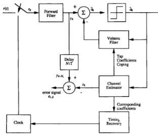
signal is then in the form of a third-order binary Volterra series [lo]: T k = a k - i h l ( 2 , T ) 2 Delay NIT I U I 2 f i c i e n t s Coping

&-Zk

r p

Estimator Channel

error sienal

Corresponding cxfficients

where

++-fI

Recovery Timini

+

a k - l a k - i - l a k - i - 2 h 3 ( i , T)

+

n k (9)

k

h i ( i , T ) = p ( i T + T ) + ? ( S ’ ( Z T + T + 2 T )

Fig. 2. Volterra-DFE in conjunction with channel estimator.

4

- s’(iT

+

7-

+

T )

+

s’(iT

+

T ) } ₍₁₀₎ and

h 3 ( i , T ) = %’(iT

+

T ) ₍₁₁₎ 4

are the linear and third order nonlinear terms in the channel response, respectively.

In (5), the recording channel is assumed to be affected by the previous transition at one-bit interval earlier only. The peak position and transition width of pulse transition, however, may be effected by several earlier transitions simultaneously. Therefore, the read signal, sampled at time

kT

+

T , can be denoted as

N z - 2 N z - 1 N z

a k - i l a k - i z u k - i 3 h 3 ( i l , i 2 r i 3 7 7-1

+

n k (12) where h l ( i , T ) and h 3 ( i 1 , i 2 , i 3 , T ) are the sampled channel

response with memory containing N I precursor taps and N 2

postcursor taps, respectively.

111. NONLINEAR DECISION FEEDBACK EQUALIZATION

The block diagram of a decision feedback equalizer in

conjunction with channel estimator is shown in Fig. 2 [19].

To equalize the nonlinear distortion of the recording channel discussed in the last section, a Volterra filter is used to replace the linear transversal filter equalization in the feedback section. The nonlinear DFE denoted as Volterra-DFE is based on modeling a nonlinear channel by a Volterra series to equalize the nonlinear distortion. The output signal, &, of the Volterra- DFE is denoted as N i N z a k = T k + i f i -

[

a k - 1 b l ( i ) i=O i = l + N J 2 N J 1

5

i l = l i z = i l + l i 3 = i 2 + l ’ a k - i l a k - i z U k - i 3 b 3 ( 2 1 , i 2 , i 3 )

}

(13)

where N l and

N2

are the number of taps in the forward and

feedback sections, respectively. Moreover, the values of f i , i = 0 , 1 , 2 ,

. . . ,

N I , are the tap coefficients of the forward filter and b l ( i ) , i = 1 , 2 , . . - , N 2 , and b 2 ( i l , i 2 , 2 3 ) , l

5

i l < i a < i 3

5

N 2 , are the linear and third-order tap coefficients of the feedback Volterra filter, respectively. The number of taps in the feedback filter is equal to the time-span of IS1 in the

discrete channel model. Assuming that past decisions i i k from

the Volterra-DFE are correct, i.e., i i k = U k , the error signal

is given by e k = G k - a k N z - 2 N z - 1 { N z i = l i 1 = l i z = i x + l N i = c T k + i f i - c a k - i b l ( i )

+

i=O

5

a k - i l a k - i z a k - i 3 b 3 ( i l , i 2 , i ~ ) - a k (14) i 3 = i z + l

1

The readout signal, T k , is represented as the nonlinear

distortion of the recording system in (12). Combining (12)

and (14), the error signal e k becomes N z N i i = - N 1 j = O e k =

{

a k - i h l ( i

+

j ) f j N z - 2 N z - - l N2 N i i l = - N 1 i 2--21+1 - ’ i 3 = i 2 + l j = O

+

a k - i ~ a k - i ~ a k - i s i l = l i z = i l + l

1

Na ’ Uk-ilak-izak-i3b3(il,~2,23) - a k . (15) i 3 = i z + l

In the mean squared error (MSE) criterion, the tap coef-

LIN AND WE1 ADAFTNE NONLINEAR DECISION FEEDBACK FQUALJZATION 199

minimize the mean-squared value of the error e k , which is denoted as E[lekI2]. To minimize the MSE, the tap coefficients of the feedback filter in Volterra-DFE require that [27]

To calculate the tap coefficients of the forward filter with minimum mean square error, we take the derivative of (26)

with respect to the forward tap coefficients

f

b 3 ( 2 l , 2 2 7 2 3 ) = h3(il

+

j , 22

+

j , 23

+

j)fj

for 1

5

21

<

22

<

'i3

5

N z .

Setting the derivative to zero and solving the equation, we obtain the suboptimum tap coefficients of forward filter as

f s o p t = ( 0 : H T H i

+

a:HrH3

+

u;l)-'HTra,k. j = O

(17)

Substituting (16) and (17) into (15), the error signal becomes (29)

0 N I 0 1 Therefore, combining (29) and (26), we obtain the minimum

MSE as

ek = a k - i C h i ( i + j ) f j

+

i = - N 1 j=0

_ _

i l = - N 1 i z = i l + l i 3 = i ~ + l

N ,

ak-i, ak-i,ak-i,

2

h3(il

+

j , i 2

+

j , i 3

+

j)fj

j=O N i

+

n k + j f j - ak. (18)

j=O

To simplify the notations, we define the following vectors

(see (19)-(24) shown at the bottom of the page). where the

superscript 'T' denotes the transpose of a matrix. Therefore, after combining (18), (19), and (24), the error signal will be of the vector form

(25)

T

e k = ( a k , i H l

+

az,3H3

+

nk)f - ak and the MSE, shown in Appendix, will be denoted as

J =

f

T( g a H 1 2 TH i

+

0:HTH3

+

ai1)f

(26)

where of is the power of the write signal and 0: is the power

of the noise, respectively. Furthermore, the correlation vector,

t a & , in the right-hand side of (26) is defined as

T T

- 2 f r a , k

+

02

r a , k = E{ak,lak} = 0:

E]

.

₍₂₇₎

In (29), we can only obtain the suboptimum tap coefficients of the forward filer which must be distinguished from the optimum tap coefficient values of the linear channel,

These coefficients can also be seen as the optimum tap coefficients of the forward filter in Volterra-DFE. It is apparent

that the suboptimum tap coefficients are affected by the

unequalized nonlinear distortion, which is denoted as H 3 , in

the nonlinear channel.

To justify the theoretical computation of suboptimum tap coefficients, we use two sampled nonlinear channels, as shown in Table I. In Table I, the signal-to-nonlinear distortion ratio

(SNDR)

at the channel output is defined as

i l iz i3

It is shown that channel A has less nonlinear distortion than channel B. In this simulation, the write signal a k , which is of

h l ( N :

-

l )

I

H3 =

-I , ,

200 IEEE TRANSACTIONS ON CIRCUITS AND SYSTEMS-I1 ANALOG AND DIGITAL SIGNAL PROCESSING, VOL. 42, NO. 3, MARCH 1995 TABLE I

SAMPLED PULSE RESPONSE

Channel A Channel B 0.0051 -0.0029 0.0085 -0.0052 0.0157 -0.0104 0.0325 -0.0239 0.0797 -0.0600 -0.2150 -0.0536 -0.0174 0.0811 -0.2981 0.0419 -0.0311 0.0168 -0.0042 0.0078 -0.0050 0.0041 -0.0040 -0.0029 0.1442 0.0159 9.5777 dR

the form {+l, -l}, has been written into the channels with

signal power a:. The additive white Gaussian noise power is

assumed to be 0; = -30dB relative to 0; in the nonlinear

channel. For both channels, N I = 5 and NZ = 7.

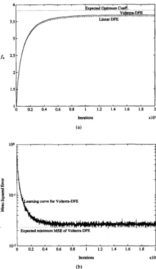
Fig. 3(a) compares the convergence of the forward tap

coefficient fo between Volterra-DFE and conventional linear

DFE in channel A. Since channel A is less impaired by the

nonlinear distortion, the convergence of the tap coefficients in Volterra-DFE and conventional linear DFE are very close to the expected optimum coefficients, as described in (31).

Fig. 3(b) shows the MSE of the Volterra-DFE. The minimum

MSE of Volterra-DFE is very close to the expected optimum

minimum MSE.

Fig. 4(a) compares the convergence of the Volterra-DFE and the conventional linear DFE in channel B. For the smaller SNDR in channel B, the tap coefficients of the Volterra- DFE and the conventional linear DFE are affected by the nonlinear distortion. They converge to two different values, as shown in the figure. In the Volterra-DFE, the tap coefficients approximate the optimum values by eliminating the tails of the

nonlinear ISI. Fig. 4(b) shows the MSE of Volterra-DFE and

the conventional linear DFE. The minimum MSE of Volterra-

DFE is shown to be smaller than the conventional linear DFE.

In Table 11, it shows the expected optimum coefficients obtained from (31) and the simulated results of the Volterra- DFE and the conventional linear DFE. In this table, the suboptimum tap coefficients of the Volterra-DFE and the conventional linear DFE are clearly shown to be affected by the nonlinear distortion. The squared error of the coefficients is defined as the summation of squared error between the expected and simulated tap coefficients. In this table, it is shown that the simulated coefficients are approximate to the

1.5

'i

I . * a . * . . . ' 0 0.2 0.4 0.6 0.8 1 1.2 1.4 1.6 1.8 2 Iterations xi04 100

4

I Iterations xi04 0 0.2 0.4 0.6 0.8 1 1.2 1.4 1.6 1.8 2 10-2 1 (b) Fig. 3.

squared of error signal ek for Volterra-DFE.

Channel A. (a) Learning curves of tap coefficient fo. (b) Mean

expected value. Comparing the minimum MSE, J m i n , of

channel A and B, it is apparent that the effect of nonlinear distortion will be dominant on the nonlinear channel. In Table

11, we define the gain of the Volterra-DFE as

gain = Jmin L/Jmin v (33)

where Jmin

v

and Jmin L are the expected minimum MSE of the

Volterra-DFE and the conventional linear DFE, respectively. It is shown that the Volterra-DFE has approximately 1.2 dB gain in the high nonlinear distortion channel.

IV. CHANNEL ESTIMATION

In the Volterra-DFE, the elimination of the tails of IS1 in the readout signal requires knowledge of the equivalent

discrete-time channel response. To accommodate a channel

that is unknown or slowly time-varying, one may include a channel estimator in parallel with the feedback filter of DFE,

as shown in Fig. 2 [ 191. The nonlinear channel estimator, using

a Volterra filter, is identical in structure to the Volterra-DFE. In fact, the nonlinear channel estimator is a replica of equivalent

LIN AND WE1 ADAPTIVE NONLINEAR DECISION FEEDBACK EQUALIZATION 4 - 3.5 3 - 20 1

-

4.5

Expected Optimum Coeff.

Voltrrra-DFE Expected Simulated 3.6804 3.688485 -1.8292 - 1.8 12889 0.0404 0.041402 0.0065 0.025739 -0.0670 -0.073076 0.0010 0.026131 0.0233 0.0264 0.0014 Line= DFE Expected Simulated 3.6532 3.653829 -1.8322 - 1.924830 0.0287 0.029323 0.ooOS 0.014580 -0.0713 -0.078235 -0.0068 0.017377 0.0260 0.0298 0.00086(18 I 0 02 0.4 0.6 0.8 1 1.2 1.4 1.6 1.8 2 Itemions XIO' (a) i 0 1 2 3 4 5 Jmin LOO

Expcctcd minimum MSE of Voltma-DFE

Expcctcd minimum MSE of linear DFE

'E

B B f 10' 0 0.2 0.4 0.6 0.8 1 1.2 1.4 1.6 1.8 2 3.7024 -1.8573 0.0527 -0.0065 -0.0621 -0.0048 0.0179 Itelations x10' (b) Fig. 4.

squared of error signal ek for DFE's.

Channel B. (a) Learning curves of tap coefficient fo. (b) Mean

Volterra-DFE

discrete-time channel filter that models the IS1 at the output

of the forward filter. The estimated channel tap coefficients

are adjusted to minimize the MSE between the output of the

estimator and the readout signal.

In Fig. 2, the estimated data sequence is fed back to the

channel estimator, which is modelled by a Volterra filter, and

the output signal Zk is given by

Linear DFE

L L - 2 L - 1 L

Zk = C a k - i c l ( i )

+

i=O i l = O i z = i l + l i 3 = i z + 1

' a k - i , a k - i z C 3 ( i l , i 2 , i 3 ) (34)

where L is the estimated tap number which is assumed to

be optimum for L = N I

+

N2. Also, c l ( i ) , 0

5

i

5

L and

C 3 ( i l , i 2 , i 3 ) , 0

5

i l < i 2

<

i 3

5

L are the tap coefficients of

the channel estimator. When DFE is used to eliminate the tails

of ISI, the channel response at the output of the forward filter

must be known a priori. Then the channel estimator is used

to minimize the mean squared value of the difference between the output signal Zk and the output signal yk of the forward

TABLE I1

(a) OPTIMUM, SUBOPTIMUM TAP COEFFICIENTS OF FORWARD FILTER

IN DFE FOR CHANNEL A. (b) OPTIMUM, SUBOPTIMUM TAP

COEFFICIENTS OF FORWARD FILTER IN DFE FOR CHANNEL B.

(a)

I I I

timum

P-7

I i l

I

Expected

I

Simulated

I

Expected

I

Simulated

I

p

_-0.6534

3

I

0.3582

I

0.8394

I

0.820823

I

0.8415

!

0.867816

I

SE of Coeff. Gain

filter. A delayed replica of the output signal yk of the forward

filter is given by

L - 2 L-1 L NI

+

a k - i l a k - i 2 a k - i 3 x

j=O

(35)

In ( 3 3 , it shows that the tap coefficients of channel estimator

will be used to estimate the precursor and post cursor IS1 of

the overall channel. That is, the delay element is equivalent to the precursor NI in the estimated tap coefficients of the channel estimator.

Assuming that the past decision sequence is correct, the

MSE is given as

202 IEEE TRANSACTIONS ON CIRCUITS AND SYSTEMS-I1 ANALOG AND DIGITAL SIGNAL PROCESSING, VOL. 42, NO. 3, MARCH 1995 Thus, supposing that the channel estimator is truly replicating

the channel response, the minimum MSE will be the filtered noise given as

The tap coefficients of channel estimator are often used to find the equivalent discrete-time channel response at the output of the forward filter. Furthermore, the feedback filter of DFE is used to eliminate the tails of IS1 on the channel. It is found that the tap coefficients of the channel estimator will be the same as the tap coefficients of the feedback filter, i.e.,

Notice that these tap coefficients of the Volterra-DFE can be copied from the corresponding tap coefficients of the channel estimator. The tap adaptation on the feedback filter of the Volterra-DFE can be saved.

V. TIMING RECOVERY

A. Sampling Phase and Volterra-DFE

In (12), the sampled channel response hl and h3 are

dependent on the sampling phase 7. The minimum MSE of

the Volterra-DFE, described in (30), will also be a function of sampling phase. This will effect the minimum MSE when the sampling phase is not optimum. To examine the performance of the DFE, it is helpful to define the output SNR as [19]

(40) 1 - Jmin

SNR=

-

Jmin

where the appropriate J m i n is obtained from the convergence

residual MSE of the DFE.

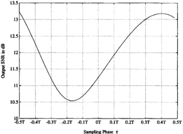
Fig. 5 shows the output SNR of a Volterra-DFE versus

sampling phase T in a nonlinear recording channel. The small

affects of nonlinear distortion in the recording channel with

normalized density S = pwSO/T = 2.5 is considered. A

pulse shift 0.1T is assumed when two consecutive adjacent transitions occur at one-bit interval earlier in the recording channel. The input SNR of the nonlinear channel is 24 dB. In this case, three forward taps and seven feedback taps are considered to be suitable for this channel. For different

sampling phase T , it is shown that the output SNR of DFE has

up to 3 dB performance loss from its maximum value. Since the result of the output SNR on the DFE varies with sampling phase, the timing recovery circuit is moderated for the optimum sampling phase to achieve the best performance. In the next section, we propose a timing recovery method in conjunction with a channel estimator to reduce the effects of nonlinear distortion.

13.5

10.5 -

10 0.5T 0.4T 0.3T 0.2T -0 1T OT 0.1T 0.2T 03T 04T 05T

SamplingPhase r

Fig. 5. Output SNR of Volterra-DFE versus sampling phase.

B. Timing Recovery and Channel Estimation

The best sampling phase for a given system depends on the overall impulse response and thus on the characteristic of the recording channel. Mueller and Muller [22] described that, depending on the pulse shape, the timing function can be defined as a linear combination of the channel impulse response:

9(.) = % h l ( i , .) (41)

where ui are scalars, h l ( i ) is the sampled impulse response of the channel. The timing function (41) will determine the transfer characteristic of the sampling clock control loop. It will be the one for which g ( 7 ) = 0 on the steady-state sampling phase. However, the channel impulse response is unknown, the timing information must be extracted from the estimated channel impulse response or from the received signal.

The timing function defined by (41) depends on the shape of impulse response of the channel to choose the right timing phase. In the recording channel, the Lorentzian-like channel response, however, can be considered as an even symmetric function about its maximum value [2]. Therefore, the timing function can be defined as

(42) In (42), the equivalent discrete-time channel response must be known a priori. Gottlieb [24] proposed a timing recovery circuit in which the timing function is extracted from the channel estimator. Therefore, the estimated channel response will be used in (42) for which each estimated tap coefficient c l ( i ) is denoted as 9(.) = h ( 1 , .) -

h ( - L

.) NI j=O c l ( i , 7) = h l ( i - N I

+

j , ~ ) f j for

o

5

i

5

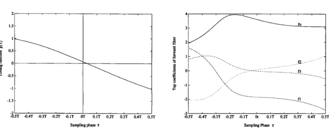
L. (43) From (43), an approximate timing function can be defined directly as [24]

LIN AND WEI: ADAPTIVE NONLINEAR DECISION FEEDBACK EQUALIZATION

2

-0.5T -0.4T 0.3T 4.2T 0.1T OT 0.1T 0.2T 0.3T 0.4T 0.5T Samplingphase z

Fig. 6. Timing function of Volterra-DFE with fixed coefficients of forward filter.

NI = f o ( h l ( L T ) - h ( - l , T ) )

+

j=1

.

@l(j

+

1 1 7 ) - h l ( j

-

1 , T ) ) f j (44) where the residual term C:!,(hl(j

+

1 , ~ )

-

h l ( j - 1 , ~ ) ) f j

is a disturbance on the timing function. Fig. 6 shows the timing function versus sampling phase. In this figure, the tap coefficients f j of the forward filter is obtained by (29) in which

the channel response H1 and H3 are fixed at the maximum

cursor of the channel response.

Since the channel estimator is placed after the forward filter of the DFE, the shape of estimated channel response will be affected by the response of the forward filter. That is, the tap coefficients of the forward filter in Volterra-DFE are also a function of the sampling phase. Thus, the shape of the channel estimator is affected by both of the channel response and forward filter of the DFE. For example, consider a nonlinear recording channel in (9) with h l ( t ) and h 3 ( t ) denoted as

h l ( t ) = 0 . 5 * ( s ( t ) - s ( t

-

T ) )

+

0 . 2 5 * ( d ( t - 2 T ) -

d ( t -

T )

+

d ( t ) )

(45)

h3(t) = 0.25*s'(t) (46)

where s ( t ) is the transition response described in (2), and

S = p w 5 0 / T = 2.5. The tap coefficients of the forward filter

in the Volterra-DFE are shown in Fig. 7. From the results of

Fig. 7, the timing function versus the sampling phase is shown

in Fig. 8. It can be seen that the timing function defined by (44) has a zero-crossing point corresponding to the maximum point of the channel pulse response.

VI.

COMPUTER

SIMULATION

In the computer simulations, a NRZI code is used as the

modulation code for the recording channel. A normalized

recording density S = 2.5 is used on the simulation channel.

The nonlinear channel assumes that a pulse shift E and a

pulse shape changing factor ,B occur between two successive

transitions. In all simulations, the signal-to-noise ratio (SNR) is chosen to be 24 dB in the recording channel. The DFE has

3 " " ' * " "

-0.5T -0.4T -0.3T -0.n -0.1T 01 0.1T 0.2T 0.3T 0.4T (

samplingphase z

Fig. 7. Tap coefficients of forward filter versus sampling phase.

0.5

203

T

0.5T -0.4T 0.3T 0.n -0.1T OT 0.1T 0.2T 0.3T 0.4T 0.5T

Sampling phase z

Fig. 8. Timing function of Volterra-DFE.

three taps in the forward filter and seven taps in the feedback filter. Only one tap of the precursor is estimated by the channel estimator, i.e., the overall size of the channel estimator is nine taps.

In Volterra-DFE with a channel estimator, the tap co- efficients of the filter are adjusted to minimize the MSE

recursively. The well known LMS algorithm [28] is used to

adapt the tap coefficients:

(47)

Cl(2,

k

+

1 ) = C l ( 2 , k )

+

2plec,kak-i

c g ( i i , iz, 23,

k

+

1 ) = c g ( i i , i 2 , i 3 ,

k)

+

2pnec,kak-ilak-izak-i~ (48) where ec,k is the error signal of channel estimator; p~ and

p n are the step-sizes of the linear and nonlinear coefficients, respectively. Meanwhile, the forward filter of the Volterra-DFE is adapted by the algorithm

fi(k

+

1) fi(k)

+

2plekrk+i (49)

where ek is the error described in (15). Furthermore, the tap

coefficients of the feedback Volterra filter are copied from the tap coefficients of the channel estimator directly.

204 IEEE TRANSACTIONS ON CIRCUITS AND SYSTEMS-11: ANALOG AND DIGITAL SIGNAL PROCESSING, VOL. 42, NO. 3, MARCH 1995 0.4

1

0.3 0.2 c t! 2 0 -Fuk Shift 0.1T Pulsc Shift 0.3T -0.3

t

....-. - - Fuk Shift 0.5T -0.41 I 200 400 600 800 1Mx) -0.5

'

1tWatiOn.S

Fig. 9. Sampling phase trajectory of Volterra-DFE.

14 13 - 12 - 11 sold Voltem-DFE - 1 10-

g

9 - 8 - 7 - "IT 0.1T 0.2T 0.3T 0.4T 0.5T 0.6T Pulse Shift E

Fig. 10. Output SNR of DFE's.

Fig. 9 shows the sampling phase trajectory of the timing

recovery circuit. Three different pulse shifts, O.lT, 0.3T, and

0.5T, are considered in the simulation. It is shown that the steady-state sampling phase is effected by the pulse shift.

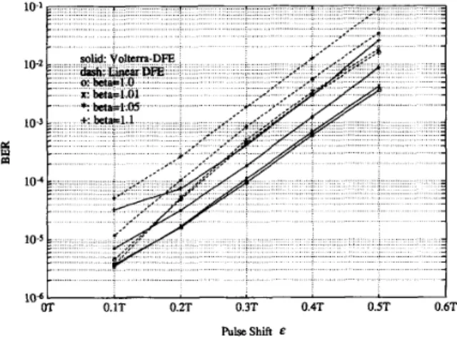
Fig. 1 0 shows the output SNR performances of the Volterra-

DFE and the conventional DFE. The pulse shift E is in the

range (O.lT, 0.5T), and /3 is in the range (1.0, 1.1). When ,8 = 1.0 means the pulse shape is not changed by the adjacent

transition. The Volterra-DFE possesses 1 dB gain in output

SNR compared to conventional DFE. The SNR gain in the Volterra-DFE, shown in Fig. 10, will improve the bit-error-

rate (BER) after the decision device, as shown in Fig. 11. It is

shown that the system with Volterra-DFE has a bit error rate one order lower than the conventional DFE when the pulse shift and pulse shape changing factor is large.

VII. CONCLUSION

The nonlinear ISI, induced by the pulse shift in a high density digital magnetic recording systems, is modelled by a Volterra filter in this paper. The Volterra-DFE, where a Volterra filter is used to replace the transversal filter in the feedback section of DFE, is introduced to eliminate the tails of

I

OT 0.1T 0.2T 0.3T 0.4T 0.5T 0.6T PulscShift E

Fig. 1 1 . BER of DFE's.

nonlinear ISI. The suboptimum tap coefficients of the forward filter in the Volterra-DFE is used to eliminate the tails of nonlinear ISI. It is found that the output SNR can be up to 3 dB different at different sampling phases. The timing recovery method based on a channel estimator is used to find the sampling phase with the best performance. To simplify the system complexity, the timing function is defined as the linear combination of tap coefficients of the channel estimator. It is shown that a timing function based on a channel estimator will operate the sampling clock on the maximum value of the main cursor. Combining the Volterra-DFE, channel estimator and timing recovery circuit, the system can combat the nonlinear distortion of the recording channel and improve the BER performance.

APPENDIX The MSE obtained form (25) is given by

J = E{lekI2} T T = E{f ( a k J H 1

+

4 3 H 3

+

nk)'

.

(a:,lHI+ 4 3 H 3

+

n k ) f } - 2E{f (akJH1

+

4 3 H 3

+

n k ) a k }

+

.g

= f T ( H T E { a k , l a : , l ) H 1

+

H m a k , 3 a : , , } H 3 T T

+

E{n:nk}

+

HTE{ak,la:,3}H3

+

HTE{ak,3az,1}Hl)f - 2 f T ( H T E { a k , l a k }

+

H 3 3 { a k , 3 a k } )

+

E { ~ k w c } )

+

ng. (A.1)

Equation (A.l) contains three fourth moments

E{ak,ia:,,}, E{ak,3a:,1}, and E{ak,sok}, and one sixth moment E { U ~ , ~ U ; , ~ } . The expectation being taken over the i.i.d. binary variables a k , has values f l with equal

probability. The expectation of the second order expectation can be calculated by using

E { U & } = OgSij. ('4.2) Then, we can obtain

LIN AND WE1 ADAPTIVE NONLINEAR DECISION FEEDBACK EQUALIZATION and ~ 205 REFERENCES 1

f a & = E { a k , l u k ) = 0:

[.I.].

(A.4)

Similarly, the 4th moment can be calculated directly by using ~ 9 1

E{apaqaras} = g I ( b p q b r s

+

bprbqs

+

bpsbqr

-

2bpqapraps).

04.5) The elements in the vector a k , 3 are aiajak, i

<

j

<

IC. We then obtain

E{ak,laz,3} = E{ak,3a:,1} = E{ak,3ak} = 0 (A.6) Consider the expectation E { u ~ , ~ u ~ , ~ } , the 6th moment E{apaqaraptaq~a,~},p

<

q

<

r and p’

<

q‘

<

r’. By using the relation

E { a p a q } = E { a p a r } = E{a,a,} = 0 (A.7) and

E { a p ! a q t } = E { u ~ ~ ~ , ~ } = E { u ~ J u , / } = 0 (AA) and the result from (A.5), we obtain

E { apaqarap/ Uq’ a,, }

= E { a p a p ’ } E { a q a r a q ’ a , ~ }

+

E { a p a q ~ }

.

E { a q a r a p ’ a , ~ }

+

E { a p ~ a p ’ } E { a p a q a , a , ~ }

- 2E{ UpUp’}E{ apaql}E{ U p ‘ U q ‘ }

.

E { a q a r f } E { a r a q / }

+

E{apaqr}E{aqap,}

.

E{ararl}

+

E { a p a q ~ } E { a q a r ~ } E { a r a p ~ }.

= E { a p a p ’ } E { a q a q ~ } E { a r a , ~ }

+

E { ~ p ~ p f }

(A.9) Since p

<

q

<

r and p’

<

q’

<

T ’ , the expectation value of (A.9) will be

E { u ~ u ~ u ~ u ~ ~ aqr U,) } = a:bppl S q q t & , t .

Therefore, the expectation value E { a k , 3 ~ : , ~ } will be (A.lO)

E{ak,3a:,3} = a,61. (A. 11) Finally, the MSE is obtained as

J = f ( a X H y H 1 + 0,6H:H3

+

~;.l)f - 2fTHFr,,k + a:.

(A. 12) This is the expression of (24).

I. C. Mallinson and C. W. Steele, “Theory of linear superposition in

tape recording,” IEEE Trans. Magn., vol. MAG-5, no. 4, pp. 886-890, Dec. 1969.

I. W. Cioffi, W. L. Ahbott, H. K. Thapar, C. M. Melas, and K. D. Fisher, “Adaptive equalization in magnetic-disk storage channels,” IEEE Commun. Mag., pp. 14-29, Feb. 1990.

D. A. Geroge, R. R. Browen, and J. R. Storey, “An adaptive decision feedback equalizer,” IEEE Trans. Commun., vol. COM-19, no. 3, pp. 281-293, June 1971.

J. W. M. Bergmans, “Decision feedback equalization for digital mag-

netic recording system,” IEEE Trans. Magn., vol. MAG-24, no. 1, pp. 683688, Jan. 1988.

-, “Density improvements in digital magnetic recording by deci- sion feedback equalization,” IEEE Trans. Magn., vol. MAG-22, no. 3, pp. 157-162, May 1986.

R. W. Wood and R. W. Donaldson, “Decision feedback equalization of the DC null in high-density digital magnetic recording,” IEEE Trans.

Magn., vol. MAG-14, no. 4, pp. 218-222, July 1978.

H. E. Melly and C. S. Chi, “Nonlinearity in high density digital recording,” IEEE Trans. Magn., vol. MAG-14, no. 5, pp. 746-748, Sept. 1978.

C. S. Chi, “Spacing loss and nonlinear distortion in digital magnetic recording,” IEEE Trans. Magn., vol. MAG-16, no. 5, pp. 976978, Sept. 1980.

J. W. M. Bergmans, S. Mita, and M. Izumita, “Characterization of digital recording channels,” Philips J. Res., vol. 44, pp. 57-96, 1989.

0. Agazzi, D. G. Messerschmitt, and D. A. Hodges, “Nonlinear echo cancellation of data signals,” IEEE Trans. Commun., vol. COM-30, no. P. Newhy and R. Wood, “The effects of nonlinear distortion on class IV partial response,” IEEE Trans. M a p , vol. MAG-22, no. 5, pp. 1203-1205, Sept. 1986.

C. M. Melas, P. Amett, I. Beardsly, and D. Palmer, “Nonlinear super- position in saturation of recording disk media,” IEEE Trans. Magn., vol. MAG-23, no. 5, pp. 2079-2081, Sept. 1987.

D. Palmer, P. Ziperovich, R. Wood, and T. D. Howell, “Identification of nonlinear write effects using pseudorandom sequences,” IEEE Trans.

Magn., vol. MAG-23, no. 5, pp. 2377-2379, Sept. 1987.

E. Biglieri, A. Gersho, R. D. Giltin, and T. L. Lim, “Adaptive cancella- tion of nonlinear intersymbol interference for voiceband data transmis- sion,” IEEE J. Select. Areas Commun., vol. SAC-2, pp. 765-777, Sept. 1984.

I. Pitas and A. N. Venetsanopoulos, Nonlinear Digital Filters. Boston, MA: Kluwer Academic, 1990.

J.-Y. Lin and C.-H. Wei, “A new adaptive equalizer for nonlinear channels,” in Proc. IEEE ISCAS, Singapore, June 1991, pp. 2814-2817.

K. D. Fisher, J. M. Cioffi, W. L. Abbott, and C. M. Melas, “An adaptive RAM-DFE for storage channels,” IEEE Trans. Commun., vol. COM-39, no. 11, pp. 454461, May 1991.

K. Fisher, J. M. Cioffi, and C. M. Melas, “An adaptive DFE for storage channels suffering from nonlinear ISI,” in Proc. ICC, Boston, MA, June J. G. Proakis, Digital Communications. New York McGraw-Hill, 1989.

G. E. Prescott, J. L. Hammond, and D. R. Hertling, “Adaptive estimation of transmission distortion in a digital communications channel,” IEEE

Trans. Commun., vol. COM-36, no. 9, pp. 107G1073, Sept. 1988. K. Mueller and M. Muller, “Timing recovery in digital synchronous data receivers,” IEEE Trans. Commun., vol. COM-24, no. 5., pp. 516531, May 1976.

A. Jennings and B. R. Clarke, “Data-sequence selective timing recovery for PAM-systems,” IEEE Trans. Commun., vol. COM-33, no. 7, pp. 729-731, July 1985.

J. Armstrong, “Symbol synchronization using baud-rate sampling and data-sequence-dependent signal processing,” IEEE Trans. Commun., vol. COM-39, no. 1, pp. 127-132, Jan. 1991.

A. M. Gottlieh, P. M. Crespo, J. L. Dixon, and T. R. Hsing, “The DSP implementation of a new timing recovery techinque for high-speed digital data transmission,” in Proc. ICASSP, New Mexico, USA, Apr. A. J. Armstrong, H. N. Bertram, R. D. Barndt, and J. K. Wolf, “Nonlinear effects in high-density tape recording,” IEEE Trans. Magn., vol. MAG-27, no. 5, pp. 4366-4375, Sept. 1991.

T. Inone, “Overwrite-induced bit shift in digital magnetic recording systems,” IEEE Trans. M a p , vol. MAG-27, no. 6, pp. 48284830, Nov. 1991.

11, pp. 2421-2433, NOV. 1982.

1989, pp. 1638-1642.

206 IEEE TRANSACTIONS ON CIRCUITS AND SYSTEMS-11: ANALOG AND DIGITAL SIGNAL PROCESSING, VOL. 42, NO. 3, MARCH 1995

[27] P. K. Shukia and L. F. Tumer, “Channel estimation-based adaptive DFE for fading multipath radio channels,” Proc. ZEE pr. I, vol. 138, no. 6, pp. 525-543, Dec. 1991.

[28] B. Widrow, J. M. McCool, M. G. Larimore, and C. R. Johson, Jr, “Stationary and nonstationary learning characteristics of LMS adaptive filter,” Proc. IEEE, vol. 64, no. 8, pp. 1151-1162, Aug. 1986. [29] J. E. Mazo, “Jitter comparison of tone generated by squaring and by

fourth-power circuits,” Bell Sysr. Tech. J . , vol. 57, no. 5 , pp. 1489-1498,

May-June 1978.

Jui-Yuan Lin was bom in Tainan, Taiwan, R 0 C ,

in 1963. He received the B.S degree in electronic engineenng from Tamkang University, Taipei, Tai- wan, in 1985, and the M S degree in communication engineering from National Chiao Tung University, Hsin Chu, Taiwan, In 1990

He is currently a doctoral student in electronics engineenng in National Chiao Tung University, Hsin Chu, Taiwan. His research interests include magnetic recording systems and adaptive signal processing.

Che-Ho Wei (S’73-M’76SM’87) was bom in

Taichung, Taiwan, R.O.C., in 1946. He received the B.S. and M.S. degrees in electronic engineering from National Chiao Tung University, Hsin Chu, Taiwan, in 1968 and 1970, respectively, and the Ph.D. degree in electrical engineering from the University of Washington, Seattle, in 1976.

From 1976 to 1979, he was an Associate Professor at National Chiao Tung University, where he is now a Professor with the Department of Electronics Engineering and the Institute of Electronics. During 1979-1982, he was the engineering manager of Wang Industrial Company in Taipei. He was the Chairman of the Department of Electronics Engineering of NCTU, from 1982 to 1986, and Director of Institute of Electronics from 1984 to 1989. He was on leave at the Ministry of Education and served as the Director of the Advisory Office from September 1990 to July 1992. His research interests include digital communications and signal processing, and related VLSI circuits design.

Dr. Wei was the founding chairmen of both the IEEE Circuits and Systems chapter and IEEE Communication chapter in Taipei. He is a member of Board of Govemors IEEE Circuits and Systems Society (1992-1994). He received the Outstanding Research Award in 1987-1989 and the Distinguished Research Award in 1990 and 1992 form the National Science Council, R.O.C.