探討缺陷石墨板之局部性質

(1)

國立交通大學

機械工程學系

碩士論文

探討缺陷石墨板之局部性質

Investigating Local Properties of Graphene Sheet with Defect

研究生：謝孟哲

指導教授：蔡佳霖博士

(2)

探討缺陷石墨板之局部性質

Investigating Local Properties of Graphene Sheet with Defect

研究生：謝孟哲 Student：Meng-Jhe Sie

指導教授：蔡佳霖 Advisor：Jia-Lin Tsai

國立交通大學

機械工程學系

碩士論文

A Thesis

Submitted to Department of Mechanical Engineering College of Engineering National Chiao Tung University

in partial Fulfillment of the Requirements for the Degree of Master

in

Mechanical Engineering

July 2010

Hsinchu, Taiwan, Republic of China

(3)

探討缺陷石墨板之局部性質

學生：謝孟哲

指導教授：蔡佳霖

國立交通大學機械工程學系碩士班

摘

要

本研究目的在探討具有自由面和裂紋之石墨板受到單軸拉伸載重下之

局部性質。利用分子動力模擬，可以得到石墨板受到單軸拉伸外力下，各

個碳原子的平衡位置。接著利用

Hardy，Lutsko 以及 Tsai 所提出的局部應

力公式，可以計算出石墨板之局部應力場。對於具有自由面的石墨板，研

究結果顯示在無應力(stress free)的條件下且凡德瓦爾(van der Waals)力存在

時，石墨板之自由面存在著壓縮應力，其他部分則受到些微的拉伸應力;而

在無應力(stress free)且凡德瓦爾力不存在的條件下，石墨板的每個位置均沒

有受力。

對於具有裂紋之石墨板，同樣先利用分子動力模擬得到拉伸載重下碳

原子的平衡位置。接著利用局部應力公式以及線彈性破壞力學(linear elastic

fracture mechanics)，有限元素法(finite element method)和非局部彈性理論

(non-local elasticity theory)來探討裂紋端附近的應力場。研究結果顯示，線

(4)

彈性破壞力學以及有限元素法的裂紋應力場皆顯示出應力奇異性(stress

singularity)，且在小裂紋情況下，線彈性破壞力學與有限元素法的應力場有

明顯的差異；而

Hardy 的應力場在靠近裂紋附近顯示出非局部(non-local)性

質，所得到的最大應力與非局部理論解非常近似。另外由

Hardy 的應力場，

也能直接從最大應力推導出石墨板之破壞性質。分析結果顯示，由

Hardy

應力場所得到的應力強度因子(stress intensity factor)與有限元素和線彈性破

壞力學一致；而破裂韌性(fracture toughness)在裂紋長度小於 40 個晶格時，

會隨著裂紋長度變小而降低；在裂紋長度大於

40 個晶格的時候，破裂韌性

才會趨於一個常數定值，此結果與非局部理論所推導出的結果一致。因此，

應力強度因子可有效地描述裂紋附近的應力場，而破裂韌性並不適合用來

描述具有小裂紋的破壞性質。

(5)

Investigating Local Properties of Graphene Sheet with Defect

Student：Meng-Jhe Sie 　 Advisor：Dr. Jia-Lin Tsai

Department of Mechanical Engineering

National Chiao Tung University

Abstract

This paper aims to investigate the local properties of graphene sheet with free surface or central cracks subjected to uniaxial loading. The equilibrium configuration of the graphene sheet subjected to uniaxial loading was determined through molecular dynamic (MD) simulation. For the graphene with free surfaces, three local stress formulations, i.e., Hardy, Lutsko and Tsai stress, were employed to calculate the local stress distribution near the free surfaces. It was found that when van der Waals force was present, only Hardy stress expression can describe the stress field effectively. Results indicated that the graphene sustained compressive stress on the edge and tensile stress in the interior at stress free state. On the other hand, when van der Waals force was absent, both Hardy and Tsai stress can describe the stress distribution accurately. Results showed that the graphene sustained zero stress at every position at stress free state such that the bond length did not alter.

Regarding the graphene with central cracks subjected to remote tensile loading, both the atomistic and continuum stress were employed to investigate the local stress distribution near the crack tip. For the discrete graphene sheet, Hardy and Tsai stress were adopted to calculate the near-tip stress field of the graphene in the absence of van der Waals interaction. For the continuum models, finite element method was used to calculate the stress

(6)

distribution. In order to describe the numerical results, two analytical solutions were incorporated, such as linear elastic fracture mechanics (LEFM) and the non-local elasticity solution. Results showed that for both LEFM and FEM solutions, the stress fields demonstrated the 1/ x stress singularity near the crack tip. In addition, it was found LEFM solution cannot describe the stress accurately when the crack length is small. On the other hand, atomistic stress such as Hardy and Tsai stress yielded a more reasonable finite stress near the tip. It was found that the maximum stress obtained from Hardy’s formulation was in agreement with the non-local elasticity solution, whereas Tsai’s maximum stress is larger than the analytical solution; therefore only Hardy stress field exhibited non-local attribute near the crack tip. Based on the maximum stress hypotheses, the fracture properties such as stress intensity factor and fracture toughness were deduced directly from local stress field. Results indicated that stress intensity factor derived from Hardy stress field was in agreement with the FEM and the actual solution of LEFM. On the other hand, the fracture toughness defined in LEFM is found to be cracksize dependent when the crack length is small for discrete models. For crack lengths below 40 lattices, the fracture toughness would decrease with the decrease of the crack lengths; the result was in agreement with the non-local elasticity solution. Therefore, the fracture toughness defined as a material property may not be suitable for describing fracture with small cracks.

(7)

誌謝在兩年的研究生活中，首先感謝恩師蔡佳霖博士的諄諄教誨與栽培，才能順利地完成碩士學位。在這過程中，除了學術專業上的學習，也增加了待人處事、溝通表達等軟知識的能力，讓我收穫良多。同時，感謝清華大學機械系葉孟考教授、交通大學機械系金大仁教授、蕭國模教授撥冗擔任學生口試委員，並給予學生許多寶貴的建議與指正。在實驗室的成員中，感謝世華學長除了在研究上的熱心指導，在生活上，也不吝給予任何的幫助，祝福你不論是留學或是工作上，一切順利。感謝林奕安、張乃仁學長、涂潔鳳學姐以及同梯王泰元，因為有你們的陪伴，讓我無論在研究或生活上都感到很安心，祝福你們工作及研究順利。謝謝學弟妹徐政文、黃奕嘉、洪健峰、高菁穗，因為有你們幫忙分擔實驗室的事務，才能讓我專心致力於研究，也祝福你們論文順利。此外，感謝父母親謝正雄先生與黃素鑾女士二十幾年來的栽培，在我的求學過程給予無盡的關愛與鼓勵，哥哥豪瑋給予完全的信任與支持，讓我能放心致力於研究，順利完成碩士學位。謝謝芮思一路的陪伴，從進入交大到完成學位，在我心情低落時，總是給予鼓勵打氣，在開心時與我分享笑容，因為有妳的陪伴，兩年的研究生活變得更有色彩，也祝福妳的論文一切順利。感謝一路走來，在我身旁的每個人，謝謝你們。孟哲

(8)

Table of Content 中文摘要 ………... i 英文摘要_{………... iii} 致謝 ………... _v 目錄 _{………... vi} 表目錄 ………... viii 圖目錄 _{………... ix} Chapter 1 Introduction………... 1 1.1 Research motivation…..………... 1 1.2 Paper review………. 1 1.3 Research approach……… 3

Chapter 2 Molecular dynamic simulation………... 5

2.1 Construction of atomistic structure of graphene sheet………. 5

2.2 AMBER force field……….………. 7

Chapter 3 Local stress distribution of graphene with free surfaces……...………... 11

3.1 Local stress formulations………...……….. 11

3.2 The determination of local stress employed in graphene system.……... 16

3.3 Stress distribution in the graphene with covalent bond interaction….… 18 3.4 Stress distribution in the graphene with covalent bond and vdW interaction……… 19

Chapter 4 Graphene with central cracks subjected to uniaxial loading……… 21

(9)

4.1.1 Near-tip stress field of non-local elasticity………...……… 22

4.1.2 Comparison of non-local stress fields with different distribution curves…………...………. 37

4.2 Comparison of stress fields in continuum models………... 37

4.3 Comparison of stress fields in discrete models………. 39

4.4 Characterizing the fracture properties of graphene sheet…………... 41

4.4.1 Stress intensity factor K………. 42

4.4.2 Fracture toughness KIC……….. 43

Chapter 5 Conclusions………... 46

References ………... 48

Appendix A MATLAB code of calculating non-local stress field for crack-tip problem using Gaussian function as distribution curve……….. 51

Appendix B MATLAB code of calculating non-local stress field for crack-tip problem using Triangular function as distribution curve 53

(10)

LIST OF TABLES

Table. 3.1.1 Cut-off radius corresponding to different smoothing lengths h……….……. 55

Table. 4.2.1 Dimension of finite element model with different crack lengths………...…. 55

Table. 4.2.2 Material properties of graphene sheet obtained from MD simulation…….… 55

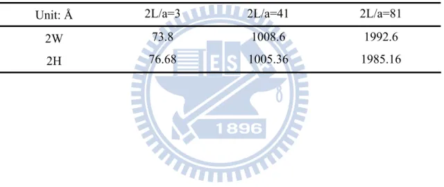
Table. 4.3.1 Different widths of discrete graphene model with crack length of 5 lattices……….…. 56

Table. 4.3.2 Dimension of discrete graphene model with different crack lengths..…...…. 56

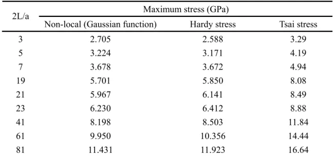
Table. 4.3.3 Maximum local stress with different crack lengths………... 57

Table. 4.4.1 Stress intensity factor from Hardy, FEM and continuum mechanics………..…….. 57

Table. 4.4.2 Stress concentration factor with different crack lengths………. 58

Table. 4.4.3 Applied loading to achieve σc with different crack lengths………. 58

(11)

LIST OF FIGURES

Fig. 3.1.1 Dimension of the dividing plane adopted in Tsai's stress

formulation………..……….…….. 60

Fig. 3.1.2 Interpretation of bond function………... 60

Fig. 3.1.3 Localization functions with various smoothing lengths……….… 61

Fig. 3.2.1 Continuous graphene sheet with periodic boundary conditions…………...….. 61

Fig. 3.2.2 Local stress in the periodic graphene with bonded interaction………... 62

Fig. 3.2.3 Hardy and Lutsko stress in the periodic graphene with bonded and

non-bonded interaction……….……….. 62

Fig. 3.2.4 Tsai stress in the periodic graphene with bonded and non-bonded interaction with different dividing planes………..……… 63

Fig. 3.2.5 Finite graphene sheet with free surfaces in the x direction………..………... 63

Fig. 3.3.1 Local stress in the finite graphene sheet with bonded interaction………... 64

Fig. 3.3.2 Bond length of finite graphene sheet with bonded interactions at stress free state……….. 64

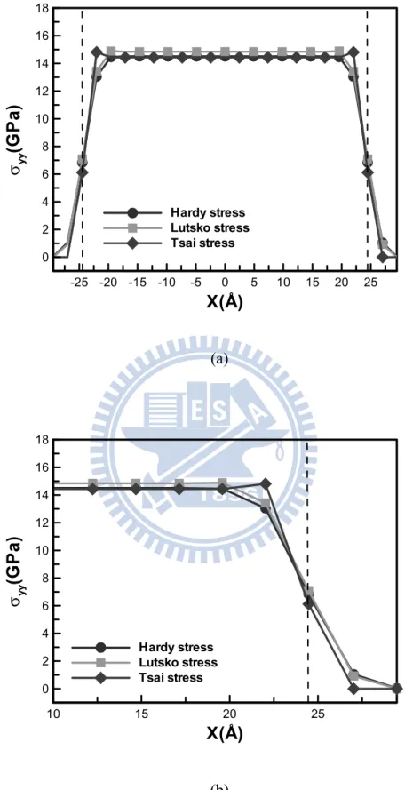
Fig. 3.3.3 Local stress distribution in the finite graphene sheet with bonded interactions (a) global view (b) local view……….. 65

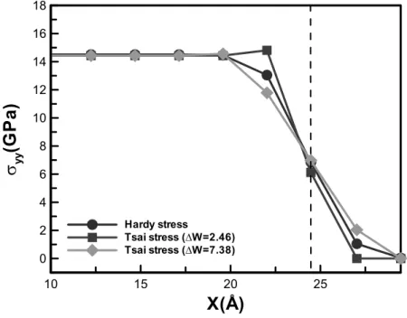
Fig. 3.3.4 Tsai stress with different dividing planes in the finite graphene sheet with bonded interactions near surface….…….………... 66

Fig. 3.3.5 Bond length of the finite graphene sheet with bonded interactions at uniaxial stress state……… 66

Fig. 3.4.1 Variation of bond length for the finite graphene sheet with bonded and non-bonded interactions at stress free state………. 67

(12)

Fig. 3.4.2 Hardy stress distribution of the finite graphene sheet with bonded and non-bonded interactions at stress free state (a) global view (b) local

view…... 68

Fig. 3.4.3 Lutsko stress distribution of the finite graphene sheet with bonded and

non-bonded interactions at stress free state………. 69

Fig. 3.4.4 Tsai stress distribution of the finite graphene sheet with bonded and non-bonded interactions at stress free state………. 69

Fig. 3.4.5 Hardy stress distribution of the finite graphene sheet with bonded and non-bonded interactions at uniaxial stress state (a) global view (b) local view…... 70

Fig. 3.4.6 Variation of bond length for the finite graphene sheet with bonded and non-bonded interactions at stress state of 10GPa………..……….. 71

Fig. 3.4.7 Lutsko stress distribution of the finite graphene sheet with bonded and non-bonded interactions at uniaxial stress state……….. 71

Fig. 3.4.8 Tsai stress distribution of the finite graphene sheet with bonded and non-bonded interactions at uniaxial stress state……….. 72

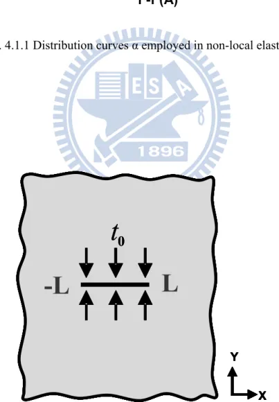
Fig. 4.1.1 Distribution curves α employed in non-local elasticity……….…….. 73

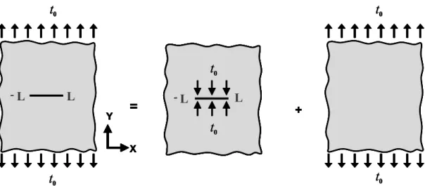
Fig. 4.1.2 Boundary conditions of the line-crack problem in non-local

elasticity………. 73

Fig. 4.1.3 Superimposition of the boundary condition in the non-local elasticity………. 74

Fig. 4.1.4 Different methods for non-local elasticity solution……… 74

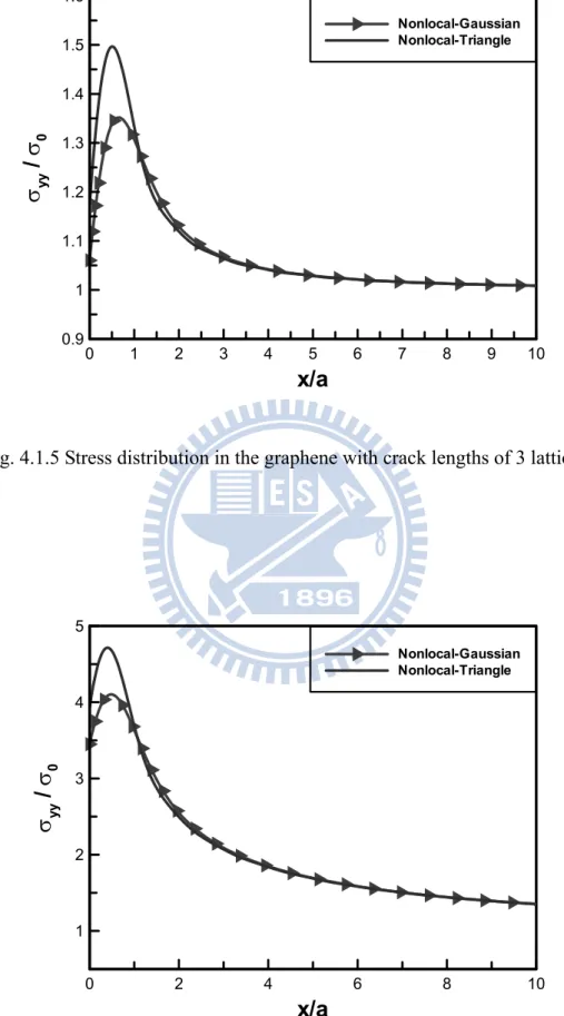
Fig 4.1.5 Stress distribution in the graphene with crack lengths of 3 lattices…………... 75

(13)

Fig. 4.2.1 Finite element model for continuum graphene sheet. Note that the dimension has different values for the three different models……….…. 76

Fig. 4.2.2 Finite element mesh for the graphene with crack lengths of 41 lattices: (a) mesh for the entire model (quarter model) and (b) magnified view of the fine mesh around the crack tip………... 77

Fig. 4.2.3 Stress distribution in the graphene with crack lengths of 3 lattices ……… 77

Fig. 4.2.4 Stress distribution in the graphene with crack lengths of 41 lattices…………... 78

Fig. 4.3.1 Atomistic structure of the graphene sheet subjected to uniaxial loading…….... 79

Fig. 4.3.2 Local stress distribution of the graphene with crack lengths of 5 lattices and different graphene widths………... 79

Fig. 4.3.3 Stress distribution in the graphene with crack lengths of 3 lattices………. 80

Fig. 4.3.4 Stress distribution in the graphene with crack lengths of 5 lattices………...… 80

Fig. 4.3.5 Stress distribution in the graphene with crack lengths of 7 lattices………..…. 81

Fig. 4.3.6 Stress distribution in the graphene with crack lengths of 19 lattices………….. 81

Fig. 4.3.7 Stress distribution in the graphene with crack lengths of 21 lattices…………... 82

Fig. 4.3.8 Stress distribution in the graphene with crack lengths of 23 lattices……….….. 82

(14)

Fig. 4.3.12 Maximum local stress in the graphene with different crack lengths…………... 84

Fig. 4.4.1

yy

xσ

π

2 plot to determine stress intensity factor of the graphene with crack lengths of 3 lattices……….. 85

Fig. 4.4.2

yy

xσ

π

2 plot to determine stress intensity factor of the graphene with crack lengths of 41 lattices……… 85

Fig. 4.4.3

yy

xσ

π

2 plot to determine stress intensity factor of the graphene with crack lengths of 81 lattice……….. 86

Fig. 4.4.4 Stress concentration factor in discrete models with different crack lengths…… 86

Fig. 4.4.5 Applied loading to achieve σc with different crack lengths………. 87

(15)

Chapter 1 Introduction 1.1 Research Motive

Graphene sheet, because of their superior mechanical performances and light weight properties, have been extensively employed in nanocomposites. This study aims to investigate the local properties of graphene sheet with free surface or central cracks. It is well known that the nanostructure of the graphene sheet may influence the mechanical performance of the nanocomposites. However, few studies have studied the local properties of the graphene sheet which are very crucial to composite design and application. In this paper, the local stress formulations, i.e. Hardy stress, Tsai stress and Lutsko stress, as well as the analytical solutions are introduced to investigate the local properties of the graphene sheet. Based on the local stress distributions, the influence of the nanostructure was characterized.

1.2 Paper Review

With the development of nanotechnology, the characterization of the mechanical properties in nano-scale is becoming an essential task and attracting lots of attention in materials community. The atomistic simulations with the advantage of simplicity have been employed to understand the fundamental mechanical properties of nanomaterials. For the nanomaterials with discreet characteristic, the stress originated based on the continuum concept would become an ambiguous physical quantity in atomistic scale. However, the determination of stress is necessary in atomistic simulation in order to correctly evaluate the mechanical properties of the materials. By considering the momentum change and the interatomistic interaction, several stress definitions suitable for the atomistic simulation have been developed. Virial

(16)

stress [1] derived from the virial theorem is first proposed and has been widely used in molecular dynamic (MD) simulations. Nevertheless, for the materials with defects or inhomogeneous deformation, only the averaged response can be demonstrated by the virial stress, and thus the “local” information which is essential in the defected material can not be clearly presented [2]. In order to modify the forward-mentioned problems, other stresses, such as Tsai stress [3], Lutsko stress [4], BDT stress [5] and Hardy stress [6] were proposed and implemented in the molecular simulation. Sun et al. [7] has systematically compared virial stress and Tsai stress and indicated that they are mathematically equivalent in calculating the overall average stress, whereas in calculating local stress distribution, virial stress exhibits unreasonable result, i.e. nonzero normal stress at free surface. As a result, Tsai's formula is more accurate than virial stress in describing the local stress field. Zimmerman and Web et al. [8, 9] based on their numerical simulations, demonstrated that Hardy stress is appropriate for both homogeneous and inhomogeneous deformation. For systems subjected to deformation, finite temperature, or both, the Hardy description of stress displays an accurate value expected from continuum theory; for the system with free surface, Hardy's expression near the surface is found to be consistent with the mechanical definition of stress. Moreover, it is very accurate and robust, and superior to BDT and Lutsko stress formulation in the local stress calculation. However, few studies concerning the local stress field of the graphene sheet with free surfaces have been reported.

One of the crucial defects in the graphene sheet is the crack, which was created during the manufacturing process. Hashimoto et al. [10] has observed several atomic defects in graphene layers by transmission electron microscopy (TEM). Meyer et al. [11] also observed some point defects in the graphene sheet by transmission electron microscopy (TEM). It seems that cracks are a common defect existing in the graphene

(17)

graphene, especially from the stress point of view. Tsai et al. [12] has adopted Hardy stress expression to investigate the local stress field of the graphene sheet with central cracks. In their study, they indicated that the stress intensity factor defined based on singular assumption may not be suitable for describing the fracture in the discrete model. Jin and Yuan [13] utilized virial stress formula to investigate the local stress field near the crack tip of the central-cracked graphene subjected to remote uniaxial loading. However, in their study, they did not discuss the local properties comprehensively. In addition, they did not demonstrate the applicability of virial stress in describing the near-tip stress field, since it is found that virial stress is inappropriate for calculating the local stress distribution [2, 7].

1.3 Research Approach

The outline of the thesis and the primary tasks of each chapter are addressed as the following. The graphene sheet with free surfaces or central cracks subjected to uniaxial loading was constructed through molecular dynamic simulation. The detail of the simulation procedures and associated potential functions and force fields were illustrated in Chapter 2.

For the graphene sheet with free surfaces, three local stress formulations, i.e., Hardy stress, Lutsko stress, and Tsai stress were introduced to investigate the local stress distribution. Graphene sheet with and without long-range interaction, i.e. van der Waals force, was discussed, respectively. In order to demonstrate the applicability of local stress formulations, a periodic single-layer graphene sheet under uniaxial loading was constructed and discussed in advance, from which the accuracy of the formulations can be verified. After the determination of local stress formulations, the local stress distribution of the graphene with free surfaces under uniaxial loading was investigated and the results were presented in Chapter 3.

(18)

In addition to the free surface, graphene sheet with central cracks subjected to remote uniaxial loading is another concern. Discrete graphene models with different central crack lengths were constructed, respectively, in which Hardy and Tsai stress expressions were employed to investigate the local stress distribution near the crack tip. For the comparing purpose, the continuum graphene models with the same geometry and line cracks were also constructed by finite element method, and the corresponding near-tip stress field was compared and discussed in detail. In order to examine the above local stress fields, two analytical solutions, i.e. linear elastic fracture mechanics and non-local elasticity solutions were incorporated. Based on the numerical and analytical results of local stress calculations, the fracture properties of the cracked graphene subjected to remote uniaxial loading can be deduced. The discussion was presented in Chapter 4.

Finally, the conclusions of the thesis were summarized in the Chapter 5.

(19)

Chapter 2 Molecular dynamic simulation

The atomistic structure of graphene sheet subjected to uniaxial loading was constructed through molecular dynamic simulations. In this chapter, the potential functions for describing the interaction between carbon atoms of graphene were presented. Two kinds of potential functions are introduced, i.e. intermolecular function and intramolecular function. Subsequently, the molecular dynamic simulation procedures were presented. The modified NPT ensemble was employed to construct the graphene sheet subjected to uniaxial loading. With the potentials and simulation procedures described, the atomistic structure of the graphene sheet subjected to uniaxial loading can be constructed accordingly.

2.1 Construction of atomistic structure of graphene sheet

Graphene is constructed by carbon atoms arranged in hexagonal pattern. The interatomistic distance between the adjacent carbon atoms is 1.42 Å, and the associated atomistic interaction is covalently bonded by SP2 hybridized electrons, the bond angle of which is 120° to each other [14]. In order to investigate the local stress field of the graphene, the atomistic structures have to be constructed in advance together with the appropriately specified atomistic interaction. In describing the graphene, two kinds of atomistic interactions are normally taken in account: one is bonded interaction, such as the covalent bond, and the other is the non-bonded interaction, i.e., van der Waals and electrostatic forces. Among the atomistic interactions, the covalent bond between two neighboring carbon atoms that provides the building block of the primary structure of the graphite may play an essential role in the mechanical responses. Such bonded interaction can be described using the potential energy that consists of bond stretching, bond angle bending, torsion, and inversion [15]. As a result, the total potential energy of the graphite contributed from

(20)

the covalent bond can be written explicitly as vdW inversion dihedral angle stretch total U U U U U U = + + + + (2.1.1)

where Ustretch is a bond stretching potential, Uangle is a bond angle bending potential, Udihedral is a dihedral angle torsional potential, and Uinversion is an inversion potential. For graphite structures under in-plane deformation, the atomistic interaction is mainly governed by the bond stretching and bond angle bending; therefore, the dihedral torsion and inversion potentials that are related to the out-of-plane deformation can be disregarded in the modeling. The explicit form for the bond stretching and bond angle bending can be approximated in terms of elastic springs as [16]

2 0) ( 2 1 ) (r k r r U_stretch _ij = _r _ij − (2.1.2) 2 0) ( 2 1 ) (θjik = θ θjik −θ angle k U (2.1.3)

where kr and kh are the bond stretching force constant and angle bending force constant, respectively. The constants kr=938 kcal/mol-Å2，kθ=126 kcal/mol-rad2 selected from AMBER force field for carbon–carbon atomic-interaction [17] are employed in the molecular simulation. The parameters r0 and θ0 represent bond length and bond angle in equilibrium position, which are assumed to be 1.42 Å and 120°, respectively, for the graphite atomistic structures. In addition to the bonded interaction, the non-bonded interaction between the carbon atoms is regarded as the van der Waals force, which can be characterized using the equivalent Lennard-Jones (L-J) potential as

(21)

⎟

⎠

⎞

⎜

⎝

⎛

−

⎟

⎠

⎞

⎜

⎝

⎛

=

₁₂ ₆

)

(

ij ij ij vdW

_r

B

r

A

r

U

(2.1.4)

where rij is the distance between the non-bonded pair of atoms. For the hexagonal graphite, the parameters A =530739.960 Å12Kcal/mole, B =343.564502Å6Kcal/mole suggested in the literature [16] were adopted in the modeling. Moreover, the cutoff distance for the van der Waals force is assigned to be 10 Å, which means that beyond this distance, van der Waals interactions are small enough to be ignored. In atomistic mechanics, all atoms except those that are bound to each other or connected to a common atom have to be accounted for in the calculation of van der Waals interactions [18].

The atomistic structures of graphene sheet with a stress-free state was obtained by performing the modified NPT ensemble with the characteristics of varying simulation box in shape and size [19] in the MD simulation at the time increment of 1 fs for 100 ps. Subsequently, the uniaxial tensile stress was applied on the graphene sheet in the y direction. After the modified NPT ensemble with time increment at 1 fs for 100 ps was performed, the deformed atomistic configuration of graphene sheet under the applied loading was obtained. It is noted that in the study, the DL-POLY package originally developed by Daresbury Laboratory [20] was modified to simulate the uniaxial loading on the graphene sheet.

2.2 Amber force field

In calculating the local stress field, one must obtain the interaction force between the atoms. Followed by the DL_POLY user manual [20], the force field derived from the above potential was presented in this section. There are three kinds of interaction force in this study.

(22)

(1) Stretching bond

The stretching bond potential between atom i and atom j is expressed as

. ) ( 2 1 ) ( 2 0 r r k r U _ij = _r _ij− (2.2.1)

Therefore the interaction force can be obtained as

( )

, h ij ij ij h ij h r r r U r U r r f ∂ ∂ ∂ ∂ − = ∂ ∂ − = (2.2.2)

where h can be atom i or atom j. The first and second term in the RHS of eqn. (2.2.2) can be expressed, respectively as

( )

₍

₎

₍

₎

0 2 0 2 1 r r k r r k r r r U ij r ij r ij ij ij ₌ ₋ ⎥⎦ ⎤ ⎢⎣ ⎡ ₋ ∂ ∂ = ∂ ∂ (2.2.3)

(

) (

)

[

]

12 1

(

2 ₂ 2

)

2 1 i i j j h ij i j i j h h ij r r r r r r r r r r r r r ∂ − + ∂ ⎟ ⎟ ⎠ ⎞ ⎜ ⎜ ⎝ ⎛ = − ⋅ − ∂ ∂ = ∂ ∂ (2.2.4) with

(

2 2 2

) (

2 2 2 2

) (

2

)

. ij ih ij jh ih i j ih i jh jh j i i j j h r r r r r r r r r r r − + = δ − δ − δ + δ = δ −δ ∂ ∂ (2.2.5)

As a result, the force field of stretching bond can be obtained as

(

₎₍

₎

. 0 ij ih ij jh ij ij r h r r r k r r f =− − δ −δ (2.2.6)

(2) Angle bending bond

(23)

. ) ( 2 1 ) ( 2 0 θ θ θ_jik = k_θ _jik − U (2.2.7)

Therefore the force exerting on atom h is

( )

, cos 1 ⎪⎭ ⎪ ⎬ ⎫ ⎪⎩ ⎪ ⎨ ⎧ ⎟ ⎟ ⎠ ⎞ ⎜ ⎜ ⎝ ⎛ ⋅ ∂ ∂ ∂ ∂ − = ∂ ∂ − = − ik ij ik ij h jik jik h jik h r r U U r r r r f θ θ θ (2.2.8)

where h can be atom i, atom j, or atom k. The first and second term in the RHS of eqn. (2.2.8) can be expressed, respectively as

( )

₍

₎

₍

₎

0 2 0 2 1 _θ _θ _θ _θ θ θ θ θ θ ⎥⎦⎤=− − ⎢⎣ ⎡ ₋ ∂ ∂ − = ∂ ∂ − _jik _jik jik jik jik _k _k U (2.2.9)

cos

{

cos

}

cos ,

1 1 1 h h ik ij ik ij h x x x x r r r r r r r ∂ ∂ ∂ ∂ = ∂ ∂ = ⎪⎭ ⎪ ⎬ ⎫ ⎪⎩ ⎪ ⎨ ⎧ ⎟ ⎟ ⎠ ⎞ ⎜ ⎜ ⎝ ⎛ ⋅ ∂ ∂ − − − _(2.2.10)

where x=cosθ. The first and second term in the RHS of eqn. (2.2.10) can be expressed as θ sin 1 1 1 cos 2 1 − = − − = ∂ ∂ − x x x (2.2.11)

( )

1 . ⎪⎭ ⎪ ⎬ ⎫ ⎪⎩ ⎪ ⎨ ⎧ ∂ ∂ ⋅ + ∂ ∂ + ∂ ∂ = ∂ ∂ ik ij h ik ij ik h ik ij ij ij h ik ij ik h r r rr r r x r r r r r r r r r r (2.2.12)

Introducing eqn. (2.2.11) and (2.2.12) into eqn. (2.2.10), one can obtain the force field of angle bending bond as

(

)

. ) ( ) ( ) cos( ) ( ) ( ) sin( 2 2 0 ⎪⎭ ⎪ ⎬ ⎫ ⎪⎩ ⎪ ⎨ ⎧ ⎥ ⎥ ⎦ ⎤ ⎢ ⎢ ⎣ ⎡ − + − − − + − − − = ik ik hi hk ij ij hi hj jik ik ij ij hi hk ik ij ik hi hj jik jik h r r r r r r k r r r r f δ δ δ δ θ δ δ δ δ θ θ θ θ (2.2.13)

(24)

(3) van der Waals force

The van der Waals potential between atom i and atom j is expressed as

. ) ( ₁₂ ₆ _⎟⎟ ⎠ ⎞ ⎜ ⎜ ⎝ ⎛ − ⎟ ⎟ ⎠ ⎞ ⎜ ⎜ ⎝ ⎛ = ij ij ij r B r A r U (2.2.14)

Therefore the interaction force can be obtained as

( )

, h ij ij ij h ij h r r r U r U r r f ∂ ∂ ∂ ∂ − = ∂ ∂ − = (2.2.15)

where h can be atom i or atom j. The first term in the RHS of eqn. (2.2.15) can be expressed as

( )

₁₂ ₆ 12 ₁₃ 6 ₇ _⎟⎟. ⎠ ⎞ ⎜ ⎜ ⎝ ⎛ − − = ⎟ ⎟ ⎠ ⎞ ⎜ ⎜ ⎝ ⎛ − ∂ ∂ = ∂ ∂ ij ij ij ij ij ij ij r B r A r B r A r r r U (2.2.16)

The second term in the RHS of eqn. (2.2.15) is identical to eqn. (2.2.4). As a result, the force field of van der Waal can be obtained as

(

)

. 6 12 ₁₃ ₇ ij ij ih ij jh h r r B r A ij ij r r f _⎟⎟ δ −δ ⎠ ⎞ ⎜ ⎜ ⎝ ⎛ − = (2.2.17)

With the force fields described above, one can employ them into the calculation of local stress.

(25)

Chapter 3 Local stress distribution of graphene with free surfaces

In this chapter, Hardy stress along with other stress formulations, such as Tsai stress and Lutsko stress were employed to calculate the local stress distribution of graphene sheet with free surfaces. The purpose of the study is to investigate the stress distribution in the vicinity of free surface such that the applicability of local stress formulations can be demonstrated when free surfaces are present. Furthermore, the effect of free surface on the morphology of the graphene sheet associated with stress distribution was discussed.

3.1 Local stress formulations

Tsai’s expression of local stress [3] is inherently the macroscopic description of stress-- the intermolecular force acting on the plane-- and at zero temperature it is expressed as , 1

_∑

∩ = A f A t δ αβ αβ δ v v _(3.1.1)

where δA denotes the area of the dividing plane and _fαβ_{is the interatomistic force} between atom α and β acting on the plane. For the graphene system, the dimension of the dividing plane adopted in the study, shown in Fig. 3.1.1, is 3.4×2.46 Å corresponding to the thickness and lattice length of the graphene. Another local stress formulation was proposed by Lutsko [21] and extended by Cormier et al. [4]. At zero temperature, it is expressed as , 2 1 1

∑∑

= ≠ Ω = N N j i avg ij r F l α β α αβ αβ αβ σ (3.1.2)

(26)

where Ω is the averaging volume, _rαβ _and _Fαβ _{represent the distance and force} between atom α and β, respectively. Moreover, _lαβ_{denotes the fraction of the length} of the α−β bond lying inside the averaging volume and its value is 0 ≤_lαβ_{≤ 1. The} averaging volume employed in the graphene is a sphere with radius of 3.4 Å. In this paper, Hardy stress formulation is the main concern and will be compared with the above formulations; therefore, in the following subsection, the Hardy formulation is briefly reviewed.

Hardy derived the stress formulation based on the three assumptions, in which the mass density, momentum density and energy density are expressed as

( )

, ( ) 1 r r r =

∑

− = a N m t ψ ρ α α _(3.1.3) ) ( ) , ( 1 r r v r p =

∑

− = a N m t αψ α α _(3.1.4)

∑

= − ⎭ ⎬ ⎫ ⎩ ⎨ ⎧ ₊ = N m t E 1 2 0 ₍ ₎ ₍ ₎ 2 1 ) , ( α α α α α _v _φ _ψ _r _r r (3.1.5)

where ρ, p and E0 represent the mass density, linear momentum and energy density, respectively; mα, vα, rα and φα represent the mass, velocity, position and potential energy of atom α, respectively. The localization function ψ serves the purpose of spreading out the properties of atoms to the space r, allowing each atom to contribute to the continuum properties. From the above equations and introducing the conservation of linear momentum, Hardy derived the local stress field in the following manner.

(27)

, ) ) ( ( ) ( ) ( 1 1

∑

= = ⎥ ⎦ ⎤ ⎢ ⎣ ⎡ ∂ − ∂ − + − = ⎟ ⎟ ⎠ ⎞ ⎜ ⎜ ⎝ ⎛ − ∂ ∂ = ∂ ∂ N N m m t t _α α α α α α α α α α α _ψ _ψ ψ r r r v v r r F r r v p (3.1.6)

where Fα is the force acting on atom α. According to an assumption made by Hardy, the force on any atom α can be written as

( ) ( .) 1 1

∑∑

∑

= ≠ = − = − N N N α β α α αβ α α α_ψ _r _r _F _ψ _r _r F (3.1.7)

Since the potential employed in the present study is in the pair-wise form, Fαβ represents the force exerted on atom α from atom β. Moreover, based on Newton’s third law, Fαβ = - Fαβ, the above equation can be rewritten as the following

∑

∑∑

[

]

= ≠ = − − − = − N N N 1 1 . ) ( ) ( 2 1 ) ( α β α β α αβ α α α_ψ _r _r _F _ψ _r _r _ψ _r _r F (3.1.8)

2. For the purpose of making the stress expression simple and plain, Hardy defined the bond function Bαβ as

, ) ( ) ( 1 0

∫

+ − ≡ ψ λ αβ β λ αβ _d B r r r r (3.1.9)

where rαβ =rα-rβ. In order to obtain some insight into the bond function, the integration can be written in the summation form

(28)

[

( ) ... ( )

]

1, ) ( ) ( 1 1 m B m m n n _r _r r r ψ λ ψ ψ αβ _≡

∑

_Δ ₌ ₊ ₊ = (3.1.10)

where r1 and rm represent rβ-r and rα-r, respectively, as illustrated in Fig. 3.1.2. From eq. (3.1.10) and Fig. 3.1.2, it is clear to see that the bond function spreads out the property of bond by dividing the length between atom α and β into several segments and allowing each segment to contribute to the space x. By taking the derivative of

ψ in eq. (3.1.9) with respect to λ

, ) ( ) ( αβ β ψ λ αβ β αβ λ λ ψ r r r r r r r r ∂ − + ∂ − = ∂ − + ∂ (3.1.11)

and integrating both sides of the above equation with respect to λ from 0 to 1, respectively, the following relation can be obtained

. ) ( ) ( ) ( r r r r r r r ∂ ∂ − = − − − β αβ αβ α _ψ ψ B (3.1.12)

Therefore, along with eq. (3.1.7) to eq. (3.1.12), the time derivative of linear momentum density can be written as

[

]

( ) . 2 1 ) ( 1 1 ⎪⎭ ⎪ ⎬ ⎫ ⎪⎩ ⎪ ⎨ ⎧ ⊗ + − ⊗ ∂ ∂ − = ∂ ∂

_∑

_∑∑

= = ≠ N N N B m t _α _α _β _α αβ αβ αβ α α α α_v _v _ψ _r _r _r _F _r r p (3.1.13)

3. From the continuum balance of linear momentum, the following relation can be obtained

(29)

(

σ v v

)

, x p ₋ _⊗ ∂ ∂ = ∂ ∂ _ρ t (3.1.14)

where σ, ρ, v denotes continuum stress, mass density and velocity, respectively. Hence eq. (3.1.13) and (3.1.14) can be connected and expressed as

(

) (

)

⎪⎭ ⎪ ⎬ ⎫ ⎪⎩ ⎪ ⎨ ⎧ ⊗ + − − ⊗ − − =

∑

∑∑

= = ≠ N N N B m 1 1 ) ( 2 1 ) ( ) ( α α β α αβ αβ αβ α α α α _v _v _v _v_ψ _r _r _r _F _r r σ (3.1.15)

where mα, vα, rα represent the mass, velocity and position of atom α, respectively; v and ψ represent the continuum velocity and localization function, respectively. It is noted that when the system is simulated at 0 K, the kinetic contribution of eq. (3.1.15) is zero. As a result, Hardy’s local stress field can be finally derived as

. ) ( 2 1 ) , ( 1 ⎟ ⎟ ⎠ ⎞ ⎜ ⎜ ⎝ ⎛ − =

∑∑

= ≠ N N j i ij t r F B α β α αβ αβ αβ σ r r (3.1.16)

From Hardy’s stress expression, one can see that the localization function plays an important role in the calculation of stress. In this study, Gaussian function with normal distribution property is employed in Hardy's formula. As a result, ψ is expressed as , ) ( exp ) ( 1 ) , ( ₂ 2 ⎟⎟ ⎠ ⎞ ⎜⎜ ⎝ ⎛₋ − = − h h h _d r r r rα α π ψ (3.1.17)

(30)

graphene sheet can be viewed as a two-dimensional system with thickness of 3.4 Å [22], d is equal to 2 in this study. The smoothing length represents the way that the properties of discrete atoms are distributed to the continuum space. Different localization functions with various smoothing lengths are shown in Fig. 3.1.3. As one can see in the figure, a short smoothing length, such as h=1.8, represents a sharp drop in distribution while a long one stands for a smoothly-decayed distribution, like h equal to 3.0. It is noted that for 2-D Gaussian function, the following relation must be satisfied,

( ) 2 1. 2 =

∫∫

x d x R ψ

(3.1.18)

Since the value of the function is approaching zero at long distances as shown in Fig. 3.1.3, for the purpose of reducing computing cost, an appropriate cut-off radius is needed in calculation. Table 3.1.1 lists the cut-off radius corresponding to each localization function with different smoothing lengths. With the cut-off radius suggested in Table 3.1.1, one can obtain a precise value with numerical error below 10-7 %. In this chapter, the smoothing length employed in Hardy’s formulation is 2.5 and the corresponding cut-off radius is 9 Å.

3.2 The determination of local stress employed in graphene system

Before applying local stress formulations to the graphene sheet with free surface, a perfect graphene sheet with periodic boundary conditions imposed in the in-plane directions was constructed through molecular dynamic simulation, such that the accuracy of local stress formulations can be verified in advance. In addition, for the purpose of showing the applicability of local stress formulations in terms of atomistic

(31)

interaction, such as covalent bond, and the other comprises bonded as well as non-bonded interactions, i.e. covalent bond and van der Waals. Followed by the procedures mentioned in the previous chapter, the atomistic structures of graphene sheet with a uniaxial stress state of 10 GPa was obtained by performing the modified NPT ensemble and then taken as an illustration as shown in Fig. 3.2.1. Fig. 3.2.2 shows the stress distribution of graphene sheet with only bonded interaction, i.e. covalent bond force field. From the figure, one can see that both Hardy and Tsai's local stress expressions demonstrate satisfactory accuracy of local stress distribution whereas a slight overestimate is found in Lutsko’s stress expression. Fig. 3.2.3 shows the stress distribution of graphene sheet with bonded as well as non-bonded interactions, calculated by Hardy and Lutsko’s formulations. It is apparent that Lutsko stress fluctuates substantially along the x axis while Hardy stress remains a uniform and precise distribution. For Tsai’s stress formula, it is seen from Fig. 3.2.4 that with the increase of the width of dividing plane, the stress tends to converge to the external applied stress, i.e. 10 GPa. It is found, however, the stress converges to 10 GPa only until the width of the dividing plane is exactly the same as the simulation box, and hence the local stress distribution can not be exhibited. Therefore, based on the above discussion, it is known that for the graphene sheet with only bonded interaction, Hardy as well as Tsai's formulations are demonstrated to be appropriate for calculation of local stress; on the other hand, for the graphene sheet with bonded interactions as well as the non-bonded interaction, due to the presence of long-range interaction from van der Waals force, only Hardy stress formulation is suitable for calculating local stress. The graphene sheet with free surface in the x direction is shown in Fig. 3.2.5 and the position for stress calculation is the x axis.

(32)

3.3 Stress distribution in the graphene with covalent bond interaction

Similar to the procedures mentioned in the pervious chapter, the associated atomistic structures of graphene sheet with free surfaces with bonded interactions at the stress free state and uniaxial stress state of 10 GPa were obtained by performing the modified NPT ensemble. When the deformed configuration of the atomistic graphene structure is derived from the modified NPT ensemble, the corresponding local stress distribution can be calculated using Hardy, Lutsko and Tsai’s stress formulations. As shown in Fig. 3.3.1, all three formulations result in a uniform zero stress at stress free state. The dotted lines marked in the figure locate the positions of the free surfaces. The corresponding morphology is shown in Fig. 3.3.2. It is apparent that with only the bonded potentials, the graphene sheet is quite stable at stress free state and hence the configuration does not alter. The stress distribution at uniaxial stress state (10 GPa) is shown in Fig. 3.3.3. It is noted that due to the difference of cross section areas between graphene sheet and simulation box, the actual load carried by the graphene is 14.4 GPa. As one can see from the figure, near the free surface, the local stress calculated from the three expressions begins to drop gradually due to the influence of free surface. The extent of the influence range from the free surface is dependent on the expression of the local stress formula. For Hardy and Lutsko stress, due to their larger radius employed in stress calculation (9Å and 3.4Å respectively), the stress drops at the position relatively far away from the surface; on the contrast, Tsai stress with smaller width of area (2.46 Å) begins to drop only at the surface. If a larger width of area (7.38 Å) is adopted in Tsai's formulation, the stress will drop at the position farther from the surface, as shown in Fig. 3.3.4. Besides, similar variation can be found in the morphology of graphene sheet, as shown in Fig. 3.3.5. Fig. 3.3.5 illustrates the elongation of bond length in the y direction along the x axis. Due to the

(33)

slightly at every position. As for the stress in the middle of the graphene, all three stress formulations result in satisfactory uniform stress distribution (14.4 GPa), except that a slight overestimate is found in Lutsko’s stress formulation.

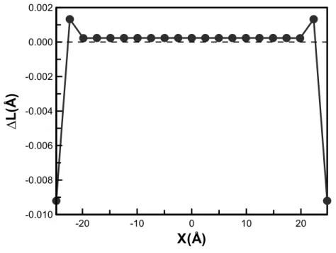
3.4 Stress distribution in the graphene with covalent bond and vdW interaction The local stress distribution in the graphene sheet with bonded and non-bonded interactions was also examined at both stress free state and uniaxial stress state. The variation of bond length at stress free state is shown in Fig. 3.4.1, in which ΔL represents the difference of bond length between graphene with and without free surfaces. It is obvious to see that the bonds at the surface are compressed while the others are elongated. Fig. 3.4.2 illustrates Hardy local stress distribution, from which, it is seen that the graphene sheet sustains compressive force in the vicinity of surfaces whereas in the middle, the graphene is under tensile loading. Besides, it is noted that near the surface, the stress increases slightly first and then drops gradually toward the surface, resulting in the distortion of configuration as found in Fig. 3.4.1. It is worthy to mention that even though the graphene does not posses zero stress at every position, the summation of stress from x=-35 to 35 along the x axis is still approximately zero at stress free state. Fig. 3.4.3 and 3.4.4 illustrate Lutsko and Tsai local stress distribution, respectively. From the figures, it is seen that the stress fluctuates substantially at every position; therefore, these two stress formulations are not suitable for describing the stress field when van der Waals is present.

Fig. 3.4.5 shows Hardy local stress distribution at uniaxial stress state of 10 GPa. Similarly, due to the difference of cross section area between the graphene sheet and simulation box, the actual load carried by graphene is 14.4 GPa. It is found that in the middle of the graphene, Hardy stress formulation results in accurate and uniform distribution; near the surface, the stress will drop gradually and the extent of

(34)

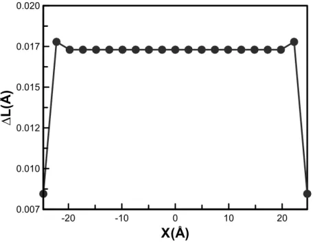
deduction and influence range are dependent on the form of localization function employed in Hardy stress expression. It can be seen that the bond length was elongated as shown in Fig. 3.4.6, due to the tensile stress existing at every position. Fig. 3.4.7 and 3.4.8 illustrate Lutsko and Tsai local stress distribution, respectively. From the figures, it is seen that the stress fluctuates substantially at every position; therefore, these two stress formulations are not suitable for describing the stress field when van der Waals is present.

(35)

Chapter 4 Graphene with central cracks subjected to uniaxial loading This chapter aims to evaluate the local stress field of the graphene sheet with central cracks subjected to remote tensile loading numerically and theoretically, from which the fracture parameters can be deduced directly. In order to validate if the fracture parameters defined in continuum fracture mechanics are still applicable for atomistic structure, both the continuum and discrete models with the same geometry and crack lengths under prescribed loading were established, respectively. The continuum model and the corresponding stress field were obtained using finite element analysis (FEA), and the analytical LEFM [23] (linear elastic fracture mechanics) solution was also incorporated. For the discrete model, the atomistic structure was constructed through MD simulation, in which Hardy and Tsai stress formulations were employed to calculate the local stress distribution. For the purpose of describing the stress field in discrete model, the non-local elasticity [24] solution was introduced. Based on the results of stress distribution, the fracture parameters concerning the linkage between the continuum and atomistic structure were obtained. In the following section, the non-local elasticity solution regarding the graphene with line crack under remote tensile loading was presented first. Subsequently, LEFM solutions as well as finite element analysis were compared and discussed. Next, the results of atomistic stress distribution in the equivalent discrete models were presented and compared with non-local elasticity solutions. Finally, the suitability of fracture parameters for characterizing the fracture behavior in atomistic structures was discussed.

4.1 Non-local elasticity in crack-tip problem

In classical elasticity, the solution of stress field in the line-crack problem of an elastic plate subject to remote uniform tension yields an infinite hoop stress at the

(36)

crack tip. In order to overcome the forward problem, Eringen [24] has proposed the non-local elasticity theory, in which the solution of stress field does not contain any singularity; instead, a finite hoop stress is found at the crack-tip such that the physical nature of the problem can be presented.

4.1.1 Near-tip stress field of non-local elasticity

The only difference between the non-local and classical elasticity is the constitutive equation and it is of the form

[

]

∫

+ = v kl kl rr kl e e dv t (r) λ' (r')δ 2μ' (r') (r'), (4.1.1)

where v is the volume occupied by the body, and

λ

'

and

μ

'

are non-local moduli and they are functions of the distance

x

'

−

x

between the reference point x and any other point x' in the body. For isotropic elastic solids, they are given by

(λ ,'μ')=(λ,μ)α

(

r'−r

)

, (4.1.2)

where α is the kernel function and is optionally given. In this study, two types of kernel function will be considered: one is the triangular-shape distribution used in Eringen's paper and the other is the Gaussian function employed previously in Hardy's formulation. For the triangular-shape distribution, it is expressed as

(

)

⎪⎩ ⎪ ⎨ ⎧ ≥ − ≤ − − − = − a r r' a r r' , r r' r r' , 0 ) (a K α (4.1.3)

(37)

where K=3/πa3 for the 2-dimensional case and a is the lattice distance. For the Gaussian function, it is expressed as

, ) ' ( exp ) ( 1 ) ( ₂ 2 2 ⎟⎠ ⎞ ⎜ ⎝ ⎛₋ − = − h h r r r r' π α (4.1.4)

where h is the smoothing length and is chosen to be 1.9 in this study. The two distributions were shown in Fig. 4.1.1. From eqn. (4.1.1), it is known that the stress tkl(r) at one point r depends on strains ekl(r') at all points r'

∈

v; as a result, the interactions with the surroundings (r') can be taken into account at the reference point r. If the following classical Hook's law is introduced

( )

r' 'kl 'rr (r') kl 2 'kl (r'),

kl σ λe δ μ e

σ ≡ = + (4.1.5)

eqn. (4.1.1) can be expressed as

.) ( ( ) ( ) ( =

∫

v kl kl dv t r α r'-r σ r' ) r' (4.1.6)

It is obvious to see that the stress at the point r is contributed from the stresses at other points r' in the body with appropriate weighting by the kernel function α. The equation of equilibrium with vanishing body force is

. 0 ) ( ( ) ( ) ( , , =

∫

= v k kl k kl dv t r α r'-r σ r' ) r' (4.1.7)

(38)

relation

( )

r'-r r')dv r')

( )

r'-r r' )dA(r'), v kl v k kl

∫

∂ = ( ( ( , α σ σ α (4.1.8)

where ∂v is the boundary surface of the body v. It is noted that when the body extends to infinity or the surface tensions are negligible, the surface integral in eqn. (4.1.8) will vanish. As a result, the remaining becomes

( )

, ( ( =0.

∫

r'-r r' )dv r') v k kl σ α (4.1.9)

Since α is an arbitrary and continuous function, eqn. (4.1.9) is satisfied if and only if

0. ) r' = ( ,k kl σ (4.1.10)

Using the classical Hook's law of eqn. (4.1.5) and the following strain tensor

(

' '

)

, 2 1 ( ' kl k,l l,k kl e u u e ≡ r')= + (4.1.11)

one can obtain the following governing equations in 2-dimensinal problems

(

)

(

)

(

)

(

)

⎪⎩ ⎪ ⎨ ⎧ = ∇ + + + = ∇ + + + . 0 ' ' ' ' 0 ' ' ' ' 2 ' ' , ' ' , 2 ' ' , ' ' , v v u u v u y y y x y x x x μ μ λ μ μ λ (4.1.12)

(39)

, ) , ( 2 1 ) , (

∫

∞ ∞ − ≡ f x y e dx y k f ikx π (4.1.13)

then the Fourier transform of eqn. (4.1.12) with respect to x' gives the following equations

(

)

(

)

⎩ ⎨ ⎧ = − + + + − = + − + + − , 0 2 ) ( 0 ) ( 2 2 ' ' , ' , ' , ' ' , 2 v k v u ik v ik u u k y y y y y y μ μ λ μ λ μ λ μ μ λ (4.1.14)

where k is the variable in the transformed domain. For the above equations, the solutions of the displacement fields can be obtained [25]

( )

ik kA k ky B k k y ikx dk ) ,y (x u ' ' 2 1/2 1 ( ) ' 3 ( ) exp( ' ') − − ⎥ ⎦ ⎤ ⎢ ⎣ ⎡ ⎟⎟ ⎠ ⎞ ⎜⎜ ⎝ ⎛ + + − + =

∫

∞ ∞ − − − μ λ μ λ π

( )

[

A k y B k

]

k y ikx dk ) ,y (x v

∫

∞ ∞ − − − − + = 2 ( ) ' ( ) exp( ' ') ' ' 1/2 π (4.1.15)

where A(k) and B(k) are two functions to be determined from the boundary conditions (Fig. 4.1.2) x = ∀ = = y t_yx σ_yx 0 0 (4.1.16) L y t tyy =− 0 =0 x < (4.1.17) . 0 0 y L v= = x > (4.1.18)

(40)

( )

2 exp( ') 2 ( ) ( ) 1 3 0. ) 0 ,' ( 1/2 _⎥ = ⎦ ⎤ ⎢ ⎣ ⎡ ⎟⎟ ⎠ ⎞ ⎜⎜ ⎝ ⎛ + + + + − − =

∫

∞ ∞ − − dk k B k kA ikx i x yx _λ _μ μ λ μ π σ (4.1.19)

Therefore, based on the above relation, B(k) can be expressed in terms of A(k) as

). ( 2 ) (k kA k B _⎟⎟ ⎠ ⎞ ⎜⎜ ⎝ ⎛ + + = μ λ μ λ (4.1.20)

The displacement fields then can be expressed as

dk k x ky ky k A y x u ( )( ')exp( ')sin( ' ) ) 2 ( ) ( 2 ) ' ,' ( 0 2 / 1 − − + + + ⎟ ⎠ ⎞ ⎜ ⎝ ⎛ − =

∫

∞ μ λ μ μ λ μ λ π (4.1.21) . ) ' cos( ) ' exp( ) ' 2 )( ( ) 2 ( ) ( 2 ) ' ,' ( 0 2 / 1 dk k x ky ky k A y x v + − + + + + ⎟ ⎠ ⎞ ⎜ ⎝ ⎛ =

∫

∞ μ λ μ μ μ λ μ λ π (4.1.22)

The remaining two boundary conditions is used to determine the unknown function

A(k). From eqn. (4.1.15),

(

)

(

) (

)

[

]

, ' ' ' , ' ' , ' ) ' ,' ( ' ' 0 0 t dy dx y y x x y y x x y x dy dx (x',y') y'-y , x'-x t yy yy yy = + − + − − = =

∫ ∫

∞ ∞ ∞ − ∞ ∞ − ∞ ∞ − α α σ σ α (4.1.23)

where σyy is expressed as

. ) ' cos( ) ' exp( ) ' 1 )( ( ) 2 ( ) ( 2 2 ) ' ,' ( 0 2 / 1 dk k x ky ky k kA y x yy ₊ + − + ⎟ ⎠ ⎞ ⎜ ⎝ ⎛ − =

∫

∞ μ λ μ λ μ π σ (4.1.24)

(41)

It is noted that for the triangular-shape distribution curve, Eringen showed the result of the integration, i.e. eqn. (4.1.23) as the following

, ) ( ) cos( ) ( ) 2 ( ) ( 2 2 0 0 2 / 1 t dk ka xk k kA t_yy = + + ⎟ ⎠ ⎞ ⎜ ⎝ ⎛ =

∫

∞ α μ λ μ λ μ π (4.1.25) where

α

is expressed as

( )

⎭ ⎬ ⎫ + − − ⎥⎦ ⎤ ⎢⎣ ⎡ − + ⎩ ⎨ ⎧ ⎥⎦ ⎤ ⎢⎣ ⎡ ₋ + ⎥⎦ ⎤ ⎢⎣ ⎡ ₊ ₋ − = − − − − 2 3 2 2 3 1 ) ( 40 ) ( 15 32 6 ) ( 20 1 3 1 ) sin( 20 1 30 19 ) cos( ) ( 20 1 15 32 30 13 6 ) ( ka ka ka ka ka ka ka ka ka ka ka π π π α Si with . sin ) ( 0

∫

= ka dt t t ka Si

For the Gaussian kernel function, the exact solution of the integration can be obtained and the detail of the derivation will be shown in the following. The boundary condition of eqn. (4.1.17) is shown again

(

) (

)

[

]

0 0 ' ' ' , ' ' , ' ) ' ,' (x y x x y y x x y y dxdy t t_yy =

∫ ∫

∞ ∞ _yy − − + − + =− ∞ − σ α α (4.1.26) where

(42)

dk k x ky ky k kA y x yy ( )(1 ')exp( ')cos( ' ) ) 2 ( ) ( 2 2 ) ' ,' ( 0 2 / 1 − + + + ⎟ ⎠ ⎞ ⎜ ⎝ ⎛ − =

∫

∞ μ λ μ λ μ π σ (4.1.27)

(

) (

)

[

]

{

}

with . 2 2 2 1 ' ' exp 1 ⎟ ⎠ ⎞ ⎜ ⎝ ⎛ = − + − − = h p y y x x p p π α

By introducing eqn. (4.1.27) into eqn. (4.1.26), one can obtain

(

) (

)

[

]

{

}

(

) (

)

[

]

{

}

' . ' dk dy dx y y x x p p k x ky ky k kA dk dy dx y y x x p p k x ky ky k kA tyy ' ' ' exp 1 ) ' cos( ) ' exp( ) ' 1 )( ( ) 2 ( ) ( 2 2 ' ' ' exp 1 ) ' cos( ) ' exp( ) ' 1 )( ( ) 2 ( ) ( 2 2 2 2 0 2 / 1 0 2 2 0 2 / 1 0 + + − − × − + + + ⎟ ⎠ ⎞ ⎜ ⎝ ⎛ − + − + − − × − + + + ⎟ ⎠ ⎞ ⎜ ⎝ ⎛ − =

∫ ∫ ∫

∞ ∞ ∞ − ∞ ∞ ∞ ∞ − ∞ π μ λ μ λ μ π π μ λ μ λ μ π (4.1.28) For the first term of eqn. (4.1.28), if the integration with respect to x' is performed first, it can be rearranged as

(

) (

)

[

]

{

}

( )

[

(

)

]

(

)

[

]

{

kx p x x dx'

}

dy'dk y y p ky ky k kA p dk dy dx y y x x p p k x ky ky k kA ' 2 0 2 2 / 1 0 2 2 0 2 / 1 0 ' exp ) ' cos( ' exp ) ' exp( ) ' 1 )( ( ) 2 ( ) ( 2 2 ' ' ' exp 1 ) ' cos( ) ' exp( ) ' 1 )( ( ) 2 ( ) ( 2 2 − − × − − − + + + ⎟ ⎠ ⎞ ⎜ ⎝ ⎛ − = − + − − × − + + + ⎟ ⎠ ⎞ ⎜ ⎝ ⎛ −

∫

∫ ∫ ∫

∞ ∞ ∞ ∞ ∞ − ∞ μ λ μ λ μ π π π μ λ μ λ μ π (4.1.29)

(43)

( )

, cos ) 4 exp( ) ( ' ) ' ( cos ) ' exp( 2 2 / 1 2 1 x p P dx x x Px I =

∫

∞ − ξ + = π −ξ ξ ∞ − (4.1.30)

one can obtain the following equation

(

)

{

}

)cos( ). 4 exp( ' exp ) ' cos( 2 2 / 1 2 kx p k p dx' x x p kx _⎟⎟ − ⎠ ⎞ ⎜⎜ ⎝ ⎛ = − −

∫

−∞∞ π (4.1.31)

As a result, eqn. (4.1.29) can be expressed as

( )

[

(

)

]

(

)

[

]

{

}

( )

[

(

)

]

dk dy kx p k p y y p ky ky k kA p dy'dk dx' x x p kx y y p ky ky k kA p ' ) cos( ) 4 exp( ' exp ) ' exp( ) ' 1 )( ( ) 2 ( ) ( 2 2 ' exp ) ' cos( ' exp ) ' exp( ) ' 1 )( ( ) 2 ( ) ( 2 2 2 2 / 1 0 2 2 / 1 0 2 0 2 2 / 1 0 ⎪⎭ ⎪ ⎬ ⎫ ⎪⎩ ⎪ ⎨ ⎧ − ⎟⎟ ⎠ ⎞ ⎜⎜ ⎝ ⎛ × − − − + + + ⎟ ⎠ ⎞ ⎜ ⎝ ⎛ − = − − × − − − + + + ⎟ ⎠ ⎞ ⎜ ⎝ ⎛ −

∫

∞ ∞ ∞ ∞ π μ λ μ λ μ π π μ λ μ λ μ π π (4.1.32)

If the integration with respect to y' is performed next, eqn. (4.1.32) can be rearranged as

( )

[

(

)

]

(

)

[

]

{

}

. dk dy' ky y y p ky p k xk k kA p p dk dy kx p k p y y p ky ky k kA p ⎭ ⎬ ⎫ ⎩ ⎨ ⎧ ₊ ₋ ₋ ₋ × − ⎟⎟ ⎠ ⎞ ⎜⎜ ⎝ ⎛ + + ⎟ ⎠ ⎞ ⎜ ⎝ ⎛ − = ⎪⎭ ⎪ ⎬ ⎫ ⎪⎩ ⎪ ⎨ ⎧ − ⎟⎟ ⎠ ⎞ ⎜⎜ ⎝ ⎛ × − − − + + + ⎟ ⎠ ⎞ ⎜ ⎝ ⎛ −

∫

∞ ∞ ∞ ∞ 0 2 2 2 / 1 2 / 1 0 2 2 / 1 0 2 2 / 1 0 ' ' exp ) ' 1 ( ) 4 exp( ) cos( ) ( ) 2 ( ) ( 2 2 ' ) cos( ) 4 exp( ' exp ) ' exp( ) ' 1 )( ( ) 2 ( ) ( 2 2 π μ λ π μ λ μ π π μ λ μ λ μ π π (4.1.33)

(44)

where

(

)

[

]

{

}

{

' ( 2 ) '

}

exp( ) 'exp

{

' ( 2 ) '

}

exp( ) .

exp ' ' exp ) ' 1 ( 0 2 2 2 0 2 0 2

∫

∞ ∞ ∞ − − − − + − − − − = − − − + k py dy' y py k py y py dy' y py k py dy' ky y y p ky

Using the following integral relations [26]

⎥⎦ ⎤ ⎢⎣ ⎡ − = − − =

∫

∞ ) 2 ( 1 ) 4 exp( ) ( 2 1 ' ) ' ' exp( 1/2 2 0 2 2 P p P dy y Py I ξ π ξ φ ξ (4.1.34) ⎥⎦ ⎤ ⎢⎣ ⎡ − − = − − =

∫

∞ ) 2 ( 1 ) 4 exp( ) ( 4 2 1 ' ) ' ' exp( ' 1/2 2 0 2 3 P p P P P dy y Py y I ξ ξ π ξ φ ξ (4.1.35) with

∫

− = − z _t _dt z 0 2 2 / 1 _exp( ₎ 2 ) ( π φ

one can obtain the following equations

{

}

⎪⎭ ⎪ ⎬ ⎫ ⎪⎩ ⎪ ⎨ ⎧ ⎥ ⎥ ⎦ ⎤ ⎢ ⎢ ⎣ ⎡ ₋ − − ⎟⎟ ⎠ ⎞ ⎜⎜ ⎝ ⎛ − = − − − −

∫

∞ ) 2 2 ( 1 ) 4 ) 2 ( exp( 2 1 ) exp( ) exp( ' ) 2 ( ' exp 2 2 / 1 2 2 0 2 p py k p py k p py py dy' y py k py φ π (4.1.36)

{

}

. ) 2 2 ( 1 ) 4 ) 2 ( exp( 4 ) 2 ( 2 ) exp( ) exp( ' ) 2 ( ' exp ' 2 2 / 1 2 0 2 2 ⎪⎭ ⎪ ⎬ ⎫ ⎪⎩ ⎪ ⎨ ⎧ ⎥ ⎥ ⎦ ⎤ ⎢ ⎢ ⎣ ⎡ ₋ − − ⎟⎟ ⎠ ⎞ ⎜⎜ ⎝ ⎛ − − − = − − − −

∫

∞ p py k p py k p p py k k p k py k py dy' y py k py y φ π (4.1.37)

探討缺陷石墨板之局部性質

國 立 交 通 大 學

機械工程學系

碩 士 論 文