在大型無線感測網路上利用小世界現象做時間同步

國

立

交

通

大

學

網路工程研究所

碩 士 論 文

在大型無線感測網路上利用小世界現象做時間同步

Small World Phenomenon for Time Synchronization in Large

Scale Wireless Sensor Networks

研 究 生：林政一

指導教授：陳 健 教授

在大型無線感測網路上利用小世界現象做時間同步

Small World Phenomenon for Time Synchronization in Large Scale

Wireless Sensor Networks

研 究 生：林政一 Student：Jeng-Yi Lin

指導教授：陳 健 Advisor：Chien Chen

國 立 交 通 大 學

網 路 工 程 研 究 所

碩 士 論 文

A Thesis

Submitted to Institute of Network Engineering College of Computer Science

National Chiao Tung University in partial Fulfillment of the Requirements

for the Degree of Master

in

Computer Science and Engineering

June 2008

HsinChu, Taiwan, Republic of China

在大型無線感測網路上利用小世界現象做時間同步

Small World Phenomenon for Time Synchronization in

Large Scale Wireless Sensor Networks

研究生 : 林政一 指導教授: 陳 健 國 立 交 通 大 學 網 路 工 程 研 究 所

摘要

近來，無線感測器網路是一個相當熱門的研究主題，由於體積小、低成本、 佈置簡單，已經有了一些實際應用，例如：物體偵測、戰場情資收集...等。然而， 這些應用都需要時間同步機制的支援，如何發展一個有效的時間同步機制是本論 文的重點。本論文改良現有的機制來完成 single-hop 時間同步，加上了小世界的 概念，來縮短 multihop 時間同步所需的時間，如此一來，不但更快完成無線感 測網路的時間同步，也可以提升時間同步的準確度。由本論文模擬結果可知，我 們所使用的方法以更快速度完成時間同步，並顯示出其方法完成 multihop 時間 同步的效能優於現有的方法。有許多人開始在水中發展無線感測網路，現今已有 許多的實際應用，例如：洋流觀測、能源探勘…等。這些應用也都需要時間同步 機制的支援。然而，在水中發展一套時間同步機制，最大的不同在於利用聲波傳 輸其速度較慢，會造成很長的傳播延遲時間(Propagation Delay)，然而現有的時 間同步機制大多假設傳播延遲時間極短可以忽略，因此無法套用在水中無線感測 網路的時間同步問題上。在本論文，我們利用 Underwater Positioning System

(UPS)[15]完成位置定位，利用位置資訊與 time difference 的技巧完成水中時間同 步。模擬結果可知，我們使用的時間同步機制，準確度可以到達

μ

s，並且可以 在應用層(Application Layer)就完成時間同步，不必再對其它層(Layers)做任何修 改。 關鍵字：時間同步、小世界、無線感測網路、有向天線、捷徑、水中時間同步、 長傳播延遲時間、聲波。

Small World Phenomenon for Time Synchronization

in Large Scale Wireless Sensor Networks

Student: Jeng-Yi Lin Advisor: Dr. Chien Chen

Institute of Computer Science and Engineering National Chiao Tung University

Abstract

Recently, the development of the wireless sensor nodes is a hot research topic. Due to its small size, low-cost and easy deployment, the sensor nodes already have many practical applications such as object detection, information gathering in battlefields…etc. However, these applications need sensor nodes have consistence in time. In this thesis, we develop several effective mechanisms for time synchronization in large-scale wireless sensor networks. Based on the existing time synchronization mechanism, coupled with the concept of small world, this thesis proposed a mechanism that can greatly reduce the time for the time synchronization in the wireless sensor networks. The result shows that our schemes can greatly reduce the time spending in the time synchronization, and shows that this methodology used in the multihop time synchronization is better than existing methods. There are so many people trying to develop a wireless sensor network for an underwater environment. There are many applications for an underwater wireless sensor network, such as

environmental monitoring, ocean current observation, energy exploration…etc. These applications need a time synchronization scheme also. However, the transmission medium is an acoustic wave that causes a long propagation time in the underwater. Nevertheless, the existing time synchronization schemes neglect the propagation time, because the propagation time is short with the electronic wave on the land. Therefore, the existing time synchronization schemes are not suitable for the underwater wireless sensor networks. In this thesis, we use the Underwater Positioning System (UPS)[15] and the technique of time difference to finish the time synchronization in a single-hop for the underwater. The simulation shows that the accuracy level is

μ

s and the time synchronization we proposed can finish the procedure in the application layer without any modification in other layers.

Keywords: Time Synchronization, Small World, Shortcut, Wireless Sensor Networks(WSN), Directional Antenna, Underwater, Long Propagation Delay, Acoustic.

誌謝

首先，要感謝的是我的指導老師陳健教授，由於老師的督促與指導才會有這 篇論文的問世。從進交大到現在，從老師身上學習到不少做研究的態度與觀念， 爾後，希望可以將這些態度與觀念繼續沿用到工作上。 此外，也感謝口試指導委員交通大學的曾煜棋教授、簡榮宏教授以及工研院 的蔣村杰博士，由於您們的指導與建議才使得本篇論文得以更臻完善。 再來要感謝的是實驗室的學長們：張哲維學長、陳盈羽學長、莊順宇學長、 周家聖學長，以及同學們：楊智強、陳信帆、王振仰、李世永、賴俊羽、陳敏正、 李致遠、黃文國、張玉奇，由於大家平時在課業上的討論與幫忙，才能讓我的研 究生涯更充實且順利。另外，也要感謝實驗室的學弟妹，希望你們可以好好把握 在交大日子，好好充實自己。 最後，最需要感謝的是我的家人與女朋友佩珊，由於你們的照顧與支持，我 才可以無後顧之憂的完成碩士學業。在此向你們致上最深的謝意。 求學生涯也將暫告一個段落，也將步入另一個人生階段。在這段漫長的求學 生涯，感謝所有師長們的教誨與指導，由於你們孜孜不倦的叮嚀與關心，才會造 就今天的我。在未來，我希望可以利用求學生涯所習得的技能與知識，秉著自身 的原則，為社會，為我的家人，為我，繼續努力下去。

Table of Content

摘要... i 

Abstract ... iii 

誌謝... v 

Table of Content ... vi 

List of Figures ... viii 

List of Tables ... x 

List of Equations ... xi 

Chapter 1: Introduction ... 1 

Chapter 2: Related Work ... 7 

2.1 Traditional Time Synchronization Method ... 7 

2.2 Non-determinism Time ... 8 

2.3 Previous Work ... 10 

Chapter 3: Small World ... 13 

3.1 Small World Phenomenon ... 13 

3.2 Firefly Phenomenon ... 14 

Chapter 4: Our Proposed Time Synchronization ... 18 

4.1 Time Synchronization in Single Hop ... 18 

4.2 Time Synchronization in Underwater ... 24 

4.2.1 Characteristic for Underwater ... 25 

4.2.2 Problem in Underwater ... 26 

4.2.3 Time Synchronization for Underwater... 29 

4.3 Time Synchronization in Multihop ... 34 

Chapter 5: Simulation and Analysis ... 50 

List of Figures

Fig. 1 Traditional Time Synchronization ... 7 

Fig. 2 OSI Architecture ... 9 

Fig. 3 Small World-Regular Graph ... 13 

Fig. 4 Small World-Small World Graph ... 14 

Fig. 5 Firefly-Local area ... 15 

Fig. 6 Firefly-The long distance communication between nodes ... 16 

Fig. 7 Firefly-Global area ... 17 

Fig. 8 RBS: Time Synchronization in Single-hop ... 19 

Fig. 9 Our method: Time Synchronization in Single-hop ... 22 

Fig. 10 Underwater-Step 1 for Time Synchronization ... 26 

Fig. 11 Underwater-Step 2 for Time Synchronization ... 27 

Fig. 12 Underwater-Step 3 for Time Synchronization ... 27 

Fig. 13 UPS ... 29 

Fig. 14 Underwater- Time Synchronization in Single-hop ... 32 

Fig. 15 RBS: Time Synchronization between Two Hops ... 35 

Fig. 16 RBS-Time Synchronization in Multihop ... 37 

Fig. 17 Transmission model-r=2, p=q=1 ... 39 

Fig. 18 Transmission Model-node A to node T ... 40 

Fig. 19 Transmission Model-Tree structure ... 41 

Fig. 20 Transmission model-RBS and RIP ... 41 

Fig. 21 Using the directional antenna to connect the node in long-distance. ... 43 

Fig. 22 Sensor Network Topology ... 43 

Fig. 23 Our method-Step 1 for Long-distance Time Synchronization ... 44 

Fig. 25 Our method-Step 3 for Long-distance Time Synchronization ... 45 

Fig. 26 Our method-Step 2 in Multihop ... 46 

Fig. 27 Our method-Step 3 in Multihop ... 47 

Fig. 28 Our method-Step 4 in Multihop ... 47 

Fig. 29 Our method-Step 5 in Multihop ... 48 

Fig. 30 Our method-Step 6 in Multihop ... 49 

Fig. 31 Convergence Time ... 52 

Fig. 32 CDF-Random Backoff Time: 0−127×20μs ... 53 

Fig. 33 CDF-Random Backoff Time: 0−511×20μs ... 53 

Fig. 34 Convergence Time: Shortcut Number Radio from 1% to 9% and Shortcut Distance from 0.10D to 0.20D ... 55 

Fig. 35 Convergence Time: Shortcut Number Radio from 10% to 90% and Shortcut Distance from 0.10D to 0.20D ... 55 

Fig. 36 CDF-Accuracy ... 57 

Fig. 37 Accuracy ... 58 

List of Tables

Table. 1 RBS-Receive Table for each node ... 19 

Table. 2 RBS-Receive Table of Node 1 ... 20 

Table. 3 RBS-Offset Table of Node 1 ... 20 

Table. 4 Our method-Receive Table for each node ... 22 

Table. 5 Our method-Time Difference Table for each node ... 23 

Table. 6 Propagation Speed ... 25 

Table. 7 Underwater-Receive Table ... 26 

Table. 8 Underwater-Time Difference Table ... 28 

Table. 9 Underwater-Receive Table for Each Node ... 32 

Table. 10 Underwater-Time Difference for Each Node ... 33 

Table. 11 RBS-Offset Value of Node 5 ... 35 

Table. 12 RBS-Offset Value of Node 4 ... 36 

Table. 13 RBS-Offset Value of Node 5 for all nodes ... 36 

Table. 14 Transmission model-Comparison ... 42 

Table. 15 Multihop-Receive Table ... 44 

List of Equations

0 1 1 T T P = −   Eq. 1 ... 8  2 3 2 T T P = −   Eq. 2 ... 8 

(

) (

)

2 2 3 0 1 T T T T − − − = α   Eq. 3 ... 8 

(

) (

)

2 2 3 0 1 T T T T − + − = β   Eq. 4 ... 8  P r r T T T T − = _ε + 2 1   Eq. 5 ... 28 

(

) (

) (

)

(

) (

) (

)

(

) (

2

) (

2

)

2 2 2 2 2 2 2 d a d a d a ad c a c a c a ac b a b a b a ab z z y y x x d z z y y x x d z z y y x x d − + − + − = − + − + − = − + − + − =   Eq. 6 ... 30  i i d sa sd ad i i c sa sc ac i i b sa sb ab t v t v d d d t v t v d d d t v t v d d d 3 2 1 Δ ⋅ = Δ ⋅ + − + Δ ⋅ = Δ ⋅ + − + Δ ⋅ = Δ ⋅ + − +   Eq. 7 ... 30  i sa i d ad i sa sd i sa i c ac i sa sc i sa i b ab i sa sb k d t v d t v d d k d t v d t v d d k d t v d t v d d 3 3 2 2 1 1 + = Δ ⋅ − − Δ ⋅ + = + = Δ ⋅ − − Δ ⋅ + = + = Δ ⋅ − − Δ ⋅ + =   Eq. 8 ... 31 

(

) (

) (

)

(

) (

) (

)

(

)

(

) (

) (

)

(

)

(

) (

) (

)

(

)

2 3 2 2 2 2 2 2 2 2 2 2 2 1 2 2 2 2 2 2 2 2 k d d z z y y x x k d d z z y y x x k d d z z y y x x d z z y y x x sa sd d d d sa sc c c c sa sb b b b sa a a a + = = − + − + − + = = − + − + − + = = − + − + − = − + − + −   Eq. 9 ... 31  2 1 2 1 r P D D r T T T T T T T = − = + = + ₋ Δ _{ε ε}   Eq. 10 ... 33  2 1 D D T T T_ε =Δ − ₋   Eq. 11 ... 34 

(

logn

)

2 =C

(

log8

)

2 =C×2.0792 =C×4.322 C   _{Eq. 12 ... 39} 

Chapter 1: Introduction

Recently, the wireless sensor networks are a hot research topic. Wireless sensor networks include many small-size and power-saving devices, normally used for sensing data and exchange information. In the wireless sensor network, a device called a node does not need a control system to control all transmission. It forms a network by itself and transmits information to remote destinations through multihop. The wireless sensor networks have some characteristics, such as limited energy consumption, high-density deployment, the implementation of low-cost, and so on. Based on the above reasons, wireless sensor network has widely be used in many applications, such as emergency applications, environmental monitoring, object detection, data collection in battlefield and monitoring system at home.

In a distributed system, time synchronization mechanism is a very important topic in wireless sensor network for the following reasons. First, they need a standard time in order to coordinate and communicate to each other. Second, the nodes must wake up and sleep at the same time for power-saving reason, so they need synchronization. Third, some scheduling algorithms such as TDMA need time synchronization, because they need to know the exact time slide to communicate information to each other. For these reasons, we must have an effective mechanism for time synchronization in order to facilitate the practical application.

There are so many people trying to develop the wireless sensor network for an underwater environment. The wireless sensor network in the underwater there are many applications, such as environmental monitoring, ocean current observation,

energy exploration…etc. These applications need time synchronization as well. The biggest difference is the transmission medium between land and underwater. There is a long propagation delay in the underwater, because the transmission medium is the acoustic wave. The speed of the acoustic wave is nearly 5 order of magnitude slower than radio on the land. The existing time synchronization schemes have a characteristic on the land, that the propagation delay is short. Therefore, we can ignore this propagation time for the time synchronization on the land. Nevertheless, the result will cause a great error, if we use the same method to finish the time synchronization in the underwater.

In the land, the most widely used scheme is NTP[1] for time synchronization in internet in wired environment. This scheme used the traditional way to achieve time synchronization. The traditional time synchronization is that two nodes transmit a packet to each other, respectively. The nodes record the transmit time and the receive time, then they can calculate the time offset for each other. It is not appropriate to the wireless sensor networks because of the non-determinism problem. The non-determinism is that the time difference between the time of the packet be construct and the time of the packet be send. In wireless sensor networks, RBS[3] proposed a scheme that can eliminate the non-determinism problem in the sender side. This method was based on the relative time difference of reference message packets arrived in each wireless sensor node. Therefore, we can get precisely time synchronization in the wireless sensor networks. In [4], they used the tree structure to achieve the time synchronization in wireless sensor networks. In [5], they greatly reduce the packet number than RBS in order to prolong the lifetime of the sensor node. The above schemes, all of them can use its methods to finish the time synchronization in single-hop. But, they usually were based on a principle that a reference node start

the procedure of the time synchronization in its transmit range. After that, a node which is picked up in this area redo the procedure in its transmit range until all nodes finish the time synchronization. Although this procedure can complete the time synchronization in multihop, they have some drawbacks. First, it needs to spend long time to finish the time synchronization in multihop, especially in large scale wireless sensor network. Second, each node has some time error because of the clock drift. Which means that the node which far away the reference node at very beginning will get more time difference than others. Therefore, we need a scheme that can reduce the hop counts in certain way.

We proposed a modified time synchronization in single-hop from RBS[3], coupled with the concept of small world. This method can greatly reduce the problem that we mentioned before. The small world phenomenon has two characteristics. The average path length (hop count) is low between the nodes in the network, and the cluster coefficient is high in the network. Small world is a phenomenon that discussed how each individual in the real world has relationships to other people. [7] performed a series of mail delivery experiments in 1967. By given receiver’s information, each individual who received this mail forwarded it to the next person according to receiver’s information such as address, career or race. In this experiment, Milgram found that an average of five and six intermediate delivers before the final receiver gets the mail. This work first quantified the famous concept of “six degrees separation” between any individual on earth. In [9][10], they further found that the cluster coefficient is good in the regular graph, but the average path length is very long. We just need to re-wired some links with the node in long-distance result in the average path length greatly reduces between the nodes. The kind of the links called shortcut. This kind of the network called a small world network.

The time synchronization in the wireless sensor network, nodes usually communicate information to each other by radio waves. In the view of small world, the link between nodes can be regarded the link as the relation between the nodes. Original idea is that how we can create a small world phenomenon in wireless sensor networks. At this moment, some nodes must have a long-distance transmission capacity that can send the packet to the node in long-distance. This called shortcut in small world. We use the directional antenna to communicate the node in long-distance to form the small world phenomenon in the large scale wireless sensor network.

The scheme we proposed is as follows: First, we randomly pick up a node that called reference node. This node broadcasts a reference packet to the neighbors within its transmission range. The nodes which receiving this reference packet can use the technique of the time difference to estimate the time offset between itself and the time server. Second, the nodes that finished the time synchronization in this area start a new round to its neighbors that did not finish the time synchronization. And, some nodes that finished the time synchronization use the directional antenna to communicate the node in long-distance to finish the time synchronization. Third, the nodes that finished the time synchronization become a time server to repeat the step 1 and 2 until the all nodes complete time synchronization. In step 2, we use the transmission model from [8]. Each node connects another node in long-distance with random way. The result shows that we can greatly decrease the hop count in the wireless sensor network.

In the underwater, [16] proposed a method that finishes the time synchronization by time-stamping the packet in the MAC layer. In [17], the author found that the

overhead is high in the previous method. The previous method will cause excessive power-consumption. The author uses mathematical analysis to find the main error source: to decrease the number of the packets in order to prolong the life cycle of the sensor node. In previous works, in order to finish time synchronization, the authors all stamp the time information in MAC layer to decrease the time error from the non-determinism time. Although, these methods can finish the time synchronization in underwater, but there is a drawback as below: we have to modify the MAC layer. Before we deploy the wireless sensor network, in order to achieve the purpose of the time synchronization, we need to modify the MAC layer. Let the packet can be stamped the time information in MAC layer before the packet be sent.

The method we proposed is as follows. First, we use the Underwater Positioning System (UPS) [15] to locate the position of each node. Second, we use the technique of the time difference to estimate the time offset between each node and the time server in order to finish the time synchronization. The biggest characteristic is that we can finish the time synchronization in the application layer without any modification in other layers.

The results show that the mechanism we proposed can greatly decrease the convergence time for the time synchronization in the large-scale wireless sensor networks. We use the directional antenna to form small world phenomenon in the wireless sensor network. Each node reduces the hop count between itself and the time server in the wireless sensor networks. In other words, the time error will be relatively lower between the nodes. In the underwater, the simulation shows that the accuracy level of the time synchronization is

μ

s and the time synchronization we proposed can finish the procedure in the application layer without any modification in other

layers.

The organization of this thesis is as follows: We discuss what is the traditional time synchronization mechanism, the problems in the traditional time synchronization mechanism, and the previous works in section 2. In section 3, we will explain the concept of small world phenomenon. In section 4, we describe that the time synchronization we proposed in more detail, including the time synchronization in the land and the time synchronization in the underwater. In section 5, we present the simulation results and analysis.

Chapter 2: Related Work

2.1 Traditional Time Synchronization Method

Before we discuss the related works, we first describe traditional time synchronization. In general, we can understand traditional time synchronization from Fig. 1.

Fig. 1 Traditional Time Synchronization

Where T0 is that node A sends a packet with time information to node B at the local time T0. T1 is that node B receives the packet from node A at the local time T1. T2 is that node B replies a packet with the time information of T0 and T1 to node A at the local time T2. T3 is that node A receives the packet with time information of T0, T1, and T2 at the time local time T3. Therefore, we can calculate the time offset

T3 T0

T2 T1

between two nodes in order to complete the purpose of time synchronization. The calculation method is easily derived as Eq. 3 or Eq. 4.

0 1 1 T T P = − Eq. 1 2 3 2 T T P = − Eq. 2

(

) (

)

2 2 3 0 1 T T T T − − − = α Eq. 3

(

) (

)

2 2 3 0 1 T T T T − + − = β Eq. 4 P: Propagation Time

α: the relative clock drift between nodes β: the propagation delay between nodes

We can easily calculate the propagation time between the node A and the node B from the difference of T1 and T0. In the same way, we can calculate the propagation time between the node A and the node B from the difference of T3 and T2. Therefore, we can average these two values to estimate the propagation time between the node A and the node B in order to get the time offset between nodes.

2.2 Non-determinism Time

Generally, there is a server that periodically sends packets to the client in traditional time synchronization. The client is using the above method to obtain the time offset with the server to finish time synchronization. Such method has a serious

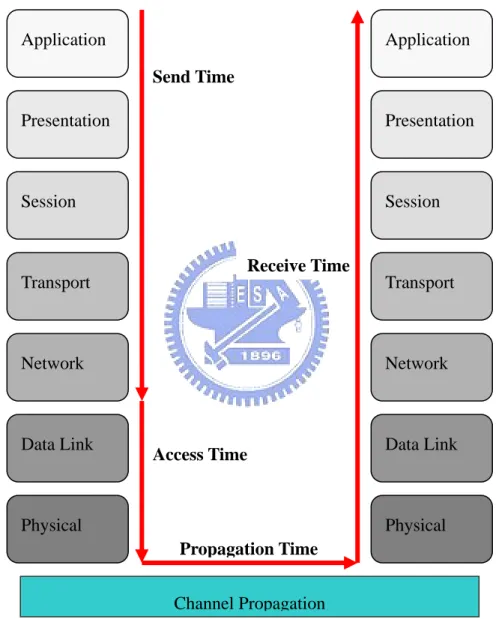
problem, which is that a long non-determinism time result in the client cannot precisely estimate the time offset between itself and the server. We will discuss is the non-determinism time in wireless sensor networks. The OSI seven-layer architecture is shown in Fig. 2.

Fig. 2 OSI Architecture

We can divide the time into four parts[6] when the server sends a packet to the receiver, as follows:

Send Time: the time spent by the sender to construct the message. Access Time Propagation Time Receive Time Send Time Application Presentation Session Transport Network Data Link Physical Channel Propagation Application Presentation Session Transport Network Data Link Physical

Access Time: delay incurred waiting for access to the transmit channel.

Propagation Time: the time needed for the message to transit from the sender to

receivers once it has left the sender.

Receive Time: processing required for the receiver’s network interface to receive

the message from the channel and notify the host of its arrival.

The time slots, as we mentioned before, greatly affect the reach time of the packet is the access time. This is called the non-determinism time. In wireless sensor networks, we usually wait for a random backoff time before the packet is send out in order to reduce the collision probability of the packets. Therefore, the arrival time of the packet from the sender to receiver is unpredictable. So, the traditional time synchronization mechanism will result in a great synchronization error.

2.3 Previous Work

In [3], the author proposed a method that can eliminate the non-determinism time error, called Reference-Broadcast Synchronization (RBS). The method shows as follows: A transmitter broadcasts m reference packets. Each of the n receivers records the time that reference was observed, according to its local clock. The receivers exchange their observations. Each receiver i can compute its phase offset to any other receiver j as the average of the phase offsets implied by each pulse received by both nodes i and j.

Using the above method, all receivers that received the reference packet is use the time of receiving packet to estimate the time offset. Therefore, we can eliminate

the time synchronization error due to the non-determinism time.

In [4], the author used the tree structure and the characteristics of RBS to develop a novel time synchronization mechanism, as follows: Construct a tree structure for all nodes. We selected a node as the reference node with tree level 0. This node broadcasts its tree level to its neighbors. The nodes that receiving this packet checks the tree level in the packet, then increase the value to become its tree level. All nodes do the same procedure until all nodes have a tree level. All nodes do the procedure of the time synchronization with its parent until all nodes finish time synchronization.

In [5], the author reduces the packet transmissions due to time synchronization mechanism in RBS. The method is as follows: The base station sends a packet to start the time synchronization. The reference node broadcasts the Reference Packet after it received the start message from the base station. Each node writes its local time received the reference packet. The base station node broadcasts the time of receipt of the reference packet. Each node interpolates its local time based on the time information broadcasted by the base station node.

The methods as we mention before can finish time synchronization in single-hop. After that, they selected a node to become the base station to do the procedure of time synchronization for its neighbors who not finish time synchronization until all nodes finish time synchronization.

With the above description, it is not difficult to find that most of time synchronization schemes do the procedure of time synchronization from specific

region to its neighbors who did not finish time synchronization until all of them are completed time synchronization. In wireless sensor networks, we usually put many sensor nodes to do a specific task. There are some problems, if we did time synchronization that likes we described before. Each node has some time drift of the clock. In large scale wireless sensor networks, because relay hop counts are too many times, we will get large time offset error between the time server and the last one that finish time synchronization when all of them finish time synchronization. We need a long period to finish the time synchronization in the large-scale wireless sensor networks. Because all of them that like we discuss before are finish the procedure of time synchronization from one specific region to another until all nodes finish the procedure.

Therefore, we proposed a novel scheme, this method can precisely finish the time synchronization in single-hop and quickly complete time synchronization in multihop with the concept of small world.

Chapter 3: Small World

3.1 Small World Phenomenon

The human can be connected by the relationship between people. The concept of small world is observed from here. In [7], the author did an experiment that we are trying to delivery a letter to someone in far place through the person we known. Each person who received this letter has to re-delivery this letter to next one who closes the receiver depending on receiver’s information through the person he known. The results show that there is about 5 or 6 times of re-delivery the letter before the letter be sent to the receiver. This phenomenon called six degree of separation.

In order to prove small world phenomenon can get how much influence in practical application. [9][10] found that we just re-wired some links in a regular graph to become a new one. The new graph can greatly reduce average path length. For example:

Fig. 3 Small World-Regular Graph

neighbors. We can calculate the shortest path between nodes in the graph by Dijakstra’s algorithm. We found that the shortest path is very long in this graph. The graph shows as follows if we re-wired some links in the graph.

Fig. 4 Small World-Small World Graph

In Fig. 4, we can observe that we greatly reduce the shortest path by Dijkstra’s algorithm due to some links are re-wired in the graph. At the same time, the connections between nodes are not change much.

In wireless sensor networks, the nodes exchange the packets of time synchronization by radio wave. Each node just connects to its neighbors. There is no long transmission capability as shortcut in small world because the transmission distance is limited. Therefore, we will use the characteristic of long-distance transmission of the directional antenna to be shortcut in small world.

3.2 Firefly Phenomenon

Except small world phenomenon, there is an interesting effect in the nature, that is firefly phenomenon. We can observe a phenomenon that is the blank of the fireflies

in the habitat. Their blanking frequency is consistence in the same area. That is means all of them adjust their blanking frequency by one of them result in the blanking frequency is consistence in the same area.

If we extend this concept to the time synchronization scheme, we can find an interesting phenomenon, as Fig. 5 shows below, where a sensor node as a firefly, the blanking behavior as the procedure of time synchronization.

Fig. 5 Firefly-Local area

In Fig. 5, each node is a firefly in the graph. Node A and node B both are the leader. The fireflies will adjust its blanking frequency nearby the leader by the blanking frequency of the leader. We can discover that the fireflies that nearby the leader form a region and the fireflies will adjust their blanking frequency by the blanking frequency of the leader. The leader B is also. In the above graph, we can think that each point is a sensor node. The node A and the node B are the reference node. The nodes around the node A and the node B will do the procedure of the time

synchronization with the reference node. After finish the time synchronization, the nodes around the node A get the time offset between itself and the node A in order to achieve the purpose of time synchronization. The nodes around the node B are also.

At this point, we can find another phenomenon, if the node A can communicate with the node B in the graph, as the Fig. 6 shows below.

Fig. 6 Firefly-The long distance communication between nodes

The firefly A is the leader of the firefly B. The firefly B adjusts its blanking frequency by the blanking frequency of the firefly A. After that, the fireflies around the firefly A and the firefly B do the procedure as we described above, as the Fig. 7 shows below.

Fig. 7 Firefly-Global area

We can find that all of the fireflies around the firefly A and the firefly B use the same frequency to flash. We can get a result that all of the nodes will get the same time offset value with a time server to achieve the purpose of the time synchronization if we use the same concept in the time synchronization scheme.

Chapter 4: Our Proposed Time Synchronization

In this chapter, we will discuss the time synchronization we proposed clearly. We will divide the time synchronization into three parts. In single-hop, we use the broadcast and the technique of the time difference to finish the time synchronization. In multihop, we use the directional antenna to connect the node in long-distance to form the small world phenomenon in wireless sensor network, and finish the time synchronization with the node in long-distance. In the underwater, we use the UPS[15] and the technique of the time difference to finish the time synchronization in single-hop.

4.1 Time Synchronization in Single Hop

In [3], we need to select a node that called reference node to broadcasts a reference packet, if we want to finish time synchronization in single-hop. The rest of nodes record the time that receiving the reference packet in the same region. After that, each node has to exchange the time information for each other in order to finish time synchronization. The nodes that get the all time information can calculate the time offset with each other by least-squares linear regression.

Fig. 8 RBS: Time Synchronization in Single-hop

Where node A is the reference node, node 1-4 are the sensor nodes.

First, the node A broadcasts a reference packet to its neighbors. Node 1-4 record the time that receiving the reference packet. If node A send the reference packet with m times, the receiving table of each node is shown as below.

1 T T 2 … Tm Node 1 Tr1,1 Tr1,2 … Tr1,m Node 2 Tr2,1 Tr2,2 … Tr2,m Node 3 Tr3,1 Tr3,2 … Tr3,m Node 4 Tr₄,1 Tr₄,2 … Tr₄,m

Table. 1 RBS-Receive Table for each node

Where T_r,b is the time of node r when it received the reference packet b

The next step, the node 1-4 exchanges its receiving table for each other. For Time

example, the receiving table of the node 1 shows as below.

1

Packet Packet2 … Packetm

Node 2 Tr2,1 Tr2,2 … Tr2,m

Node 3 Tr3,1 Tr3,2 … Tr3,m

Node 4 Tr₄,1 Tr₄,2 … Tr₄,m

Table. 2 RBS-Receive Table of Node 1

After the node 1 get the all receiving table for each node, it can calculate the time offset with each node by least-squares linear regression. The offset table is shown as below.

Offset Value

Node 2 Offset 2

Node 3 Offset3

Node 4 Offset 4

Table. 3 RBS-Offset Table of Node 1

Through the discussion as we mention before. It is not hard to find that RBS has several drawbacks. First, the number of the reference packet is too much. In order to get the time offset between itself and others, the node has to exchange the receiving table for others after the node records the time that receiving the reference packet. Therefore, the number of the packet is too much. Second, each node demands a lot of

Packet Node

Offset Node

memory size. Each node gets the time offset for each node in RBS, result in each node need a large memory size to store the related information. Third, the time to finish time synchronization is too long in single-hop. In wireless sensor networks, there is a random backoff time to reduce the collision probability before the node sends a packet to another. Each node want to send a lot of the packets to another, result in the channel is busy all the time in RBS. Therefore, each node needs more time to process the packets.

In wireless sensor networks, the nodes usually do the same task in the same region, such as object detection, information gathering in the battlefield. Base on this point, we can modify the method of RBS to fit the implementation in wireless sensor networks, the steps show as below.

Step 1. We select a reference node to broadcast a reference packet within its transmission region. The nodes that belong to this region record the time that they receive the packet.

Step 2. The node that is closest to the reference node, called the time server, replies a packet to the reference node with its receiving time on the packet.

Step 3. The reference node relays the time information to all nodes within its transmission region.

Step 4. At this point, all nodes have two time information. One is the time that it receiving the reference packet. Another one is the time that the time server receiving the reference packet. We can get the time offset between itself and the time server by the difference of two values. After we get the time offset, we can estimate the time of the time server in order to achieve the purpose of time synchronization in single-hop.

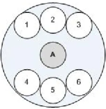
Fig. 9 Our method: Time Synchronization in Single-hop

Where node A is the reference node, the node 1-6 are the sensor nodes.

First, the node A broadcasts a reference packet within its transmission region. The nodes record the time when it receiving the reference packet. The receiving table is shown as below. T Node 1 Tr₁ Node 2 Tr₂ Node 3 T r₃ Node 4 T r₄ Node 5 T r₅ Node 6 T r₆

Table. 4 Our method-Receive Table for each node

Time Node

Assume the node 1 is the time server. The node 1 will reply a packet to the reference node with the time when it receiving the reference packet. Then, the reference node will broadcast this time information to its neighbors within its transmission region. After the step, all of nodes will get a time difference table. The table is shown as below.

T Node 2 Tr₁−Tr₂ Node 3 Tr₁−Tr₃ Node 4 Tr₁−Tr₄ Node 5 Tr₁−Tr₅ Node 6 Tr₁−Tr₆

Table. 5 Our method-Time Difference Table for each node

This table tell us, the time difference of itself and the time server when the node received the reference packet. Because the propagation time is very short, we can ignore the propagation time of the packet from one node to another. In other words, the packet almost reaches each node in the same time. After node n gets this time difference table, node n can estimate the time offset with the time server.

The algorithm we proposed has the following advantages. First, the fewer number of the packets. This algorithm just needs three packets to finish time synchronization in single-hop. Second, the memory size is smaller for each node.

Time Node

Each node just needs to record the time offset with the time server. The memory size is smaller than RBS that needs to record the time offset for all nodes. Third, this algorithm reduces the convergence time for time synchronization in single-hop. There are just three packets need to send. The nodes do not send the packet except the reference node and the time server. Therefore, this method greatly reduces the overhead for time synchronization.

Why the method we proposed, each node just needs to record the time offset with the time server? As we mention before, the nodes usually do the same tasks in the same region. We just care about the order of the events. The absolute time is not necessary. Therefore, we just need the time server to be a time standard. After all nodes finish the procedure of time synchronization. Each node can use the relative time offset of the time server to record the events. Even in the TDMA scheduling, the method we proposed is work well, because all nodes get the time offset with the time server. We can use this time information to schedule the tasks.

4.2 Time Synchronization in Underwater

In this section, we proposed a time synchronization that is suitable for the underwater environment. We use the UPS[15] and the technique of the time difference to finish the time synchronization in single-hop. We can finish the time synchronization in the application layer without any modification in other layers.

The organization of this chapter is as follows: we show the characteristic for underwater in section 4.2.1. In section 4.2.2, we will explain the problem of the time

synchronization in underwater. In section 4.2.3, we will describe the method we proposed. The simulation and analysis will be show in chapter 5.

4.2.1 Characteristic for Underwater

The biggest difference is the transmission medium between land and underwater, as the table below.

Speed of Light 3×108m /s

Speed of Sound 1500m /s

Table. 6 Propagation Speed

For this reason, the time synchronization scheme is not suitable for underwater, including [3], [4], and [5]. Because these methods have a characteristic on land, that is the packet will almost arrive to all nodes at the same time when a node broadcasts a packet to its neighbors within its transmission range. Therefore, we can ignore this error for time synchronization on the land. But, the nodes use acoustic waves to communicate with each other. The speed of sound is nearly 5 orders of magnitude slower than radio waves. If we use the same method in underwater, the result will cause a great error.

4.2.2 Problem in Underwater

If we directly apply our time synchronization to the underwater environment in single-hop, there is a problem as below.

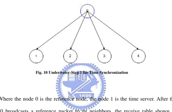
Fig. 10 Underwater-Step 1 for Time Synchronization

Where the node 0 is the reference node, the node 1 is the time server. After the node 0 broadcasts a reference packet to its neighbors, the receive table shown as below. T Node 1 T r₁ Node 2 T r₂ Node 3 T r₃ Node 4 T r₄

Table. 7 Underwater-Receive Table

Time Node

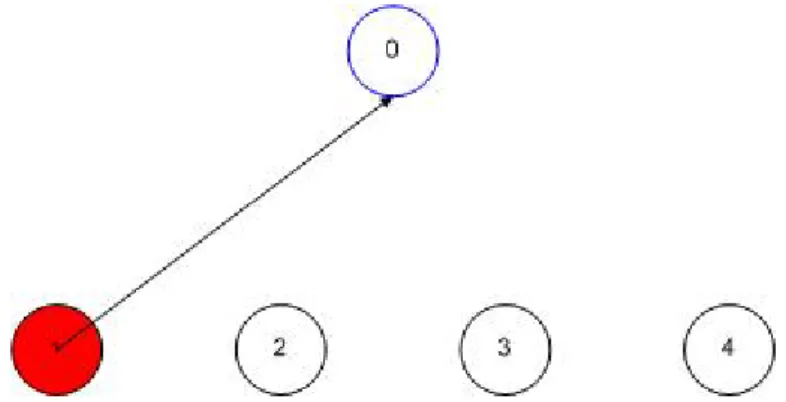
The node 1 will reply a packet with its receiving time to the node 0, after the node 1 received the reference packet, as the Fig. 11 below.

Fig. 11 Underwater-Step 2 for Time Synchronization

The node 0 will broadcast the time information of the node 1 to its neighbors, when the node 0 receives the packet from the node 1, as the Fig. 12 below.

Fig. 12 Underwater-Step 3 for Time Synchronization

After each node receives the packet with the time information of the node 1 from the node 0, the time difference table shown as below for each node.

T

Node 2 Tr₁−Tr₂

Node 3 Tr₁−Tr₃

Node 4 Tr₁−Tr₄

Table. 8 Underwater-Time Difference Table

For example, the value of the node 2 shows as below.

P r r T T T T − = _ε + 2 1 Eq. 5

Where T_ε is the time difference between two nodes, _{T is the relative P} propagation time between two nodes.

With radio communication, node 1-4 will almost get the packet at the same time that the node 0 broadcasts a packet to them. Therefore, the value of T is about 0. P

With acoustic communication, there are some differences as following. First, the transmission speed is slow. This reason causes each node to receive the broadcast packet at very different times. Second, the transmission range is longer. The transmission range can reach a few kilometers away in underwater such as [18] describes. Therefore, the value of _{T is bigger. As the above reasons, we need a new P} method to finish time synchronization in underwater, where the key point is how to calculate the time of T . P

Time Node

4.2.3 Time Synchronization for Underwater

The method we proposed can divide into two steps. First, we use the UPS system to locate the position of the node. All nodes can estimate their location in the application layer. Second, the node can calculate the time offset between itself and the time server by the time difference technique and the position information in the previous step in order to achieve the purpose of time synchronization.

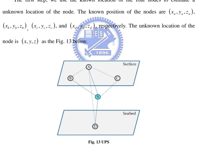
The first step, we use the known location of the four nodes to estimate a unknown location of the node. The known position of the nodes are

(

x_a,y_a,z_a

)

,

(

xb,yb,zb

)

_,

(

xc,yc,zc

)

, and

(

xd,yd,zd

)

, respectively. The unknown location of the

node is

(

x,y,z

)

_{as the Fig. 13 below.}

Fig. 13 UPS

(

) (

) (

)

(

) (

) (

)

(

) (

2

) (

2

)

2 2 2 2 2 2 2 d a d a d a ad c a c a c a ac b a b a b a ab z z y y x x d z z y y x x d z z y y x x d − + − + − = − + − + − = − + − + − = Eq. 6

Let A be the master anchor node, which initiates a beacon signal every T seconds. Each beacon interval begins when A transmits a beacon signal. Considering any beacon interval i, at time t1i,

i b

t , t , and _ci t , sensor S and anchor nodes B, C, and D _di

receive A’s beacon signal, respectively. At time t , which is _bi' ≥ t , B replies to A _bi

with a beacon signal conveying information t_bi' −t_bi =Δt_bi. This signal reaches S at time t2i. After receiving beacon signals from both A and B, at time

'

i c

t , C replies to A

with a beacon signal conveying information t_ci'−t_ci =Δt_ci. This signal reaches S at time t₃i. After receiving beacon signals from A, B, and C, at time t , D replies to A _di'

with a beacon signal conveying information t_di'−t_di =Δt_di . This signal reaches S at time t4i . Based on triangle inequality,

i i i i t t t t₁ < ₂ < ₃ < ₄ . Letting Δt1i =t2i −t1i , i i i t t t₂ = ₃− ₁ Δ , and Δt₃i =ti₄−t₁i, we obtain i i d sa sd ad i i c sa sc ac i i b sa sb ab t v t v d d d t v t v d d d t v t v d d d 3 2 1 Δ ⋅ = Δ ⋅ + − + Δ ⋅ = Δ ⋅ + − + Δ ⋅ = Δ ⋅ + − + Eq. 7 which gives

i sa i d ad i sa sd i sa i c ac i sa sc i sa i b ab i sa sb k d t v d t v d d k d t v d t v d d k d t v d t v d d 3 3 2 2 1 1 + = Δ ⋅ − − Δ ⋅ + = + = Δ ⋅ − − Δ ⋅ + = + = Δ ⋅ − − Δ ⋅ + = Eq. 8

where d_sa, d_sb, d_sc, and d_sd are positive real numbers; v is the speed of sound.

We can estimate the position of the node S by the Eq. 8 as the Eq. 9 below.

(

) (

) (

)

(

) (

) (

)

(

)

(

) (

) (

)

(

)

(

) (

) (

)

(

)

2 3 2 2 2 2 2 2 2 2 2 2 2 1 2 2 2 2 2 2 2 2 k d d z z y y x x k d d z z y y x x k d d z z y y x x d z z y y x x sa sd d d d sa sc c c c sa sb b b b sa a a a + = = − + − + − + = = − + − + − + = = − + − + − = − + − + − Eq. 9

Therefore, we can get the unknown position of the node.

For the second step, we use the technique of the time difference to finish time synchronization in single-hop. The steps are shown as below.

Step 1. Node A sends packet with its position. All nodes record the receiving time. Then, each node calculates its distance between node A and itself.

Step 2. Node 1 replies a packet with its receiving time and its distance. Step 3. Node A broadcasts this message to all nodes in its transmit range.

Step 4. Each node calculates its time offset for time server depend on these two packets.

Fig. 14 Underwater- Time Synchronization in Single-hop

Where the node A is the reference node, the node 1-6 are the sensor node.

After the node A broadcasts a reference packet to its neighbors within its transmission range, the receive table of the nodes as below.

T D Node 1 T r₁ D 1 Node 2 T r₂ D 2 Node 3 T r₃ D3 Node 4 T r₄ D 4 Node 5 T r₅ D5 Node 6 T r₆ D6

Table. 9 Underwater-Receive Table for Each Node

Assume the node 1 is the time server. The node 1 will reply a packet with its time Time

information and the distance with the node A to the node A. Then, the node A will broadcast the information to its neighbors within its transmission range. The time difference table of the nodes shown as below.

T D Node 2 Tr₁−Tr₂ D1−D2 Node 3 Tr₁−Tr₃ D1−D3 Node 4 Tr₁−Tr₄ D1−D4 Node 5 Tr₁−Tr₅ D1−D5 Node 6 Tr₁−Tr₆ D1−D6

Table. 10 Underwater-Time Difference for Each Node

Where Δ is the time difference with relative distance error between nodes, T D

Δ is the relative distance between nodes.

After above steps, we have enough information to achieve time synchronization. For example, the time difference of the node 2 is shown as below.

2 1 2 1 r P D D r T T T T T T T = − = + = + ₋ Δ _{ε ε} Eq. 10

We can get the time difference between two nodes and the relative propagation time by the Eq. 11. The relative propagation time means the propagation time between the time server and the node 2 when the reference node broadcasts a reference packet

Time Node

to its neighbors. Because the speed of sound is slow, we can calculate the relative propagation time by the position information in the step 1. For example, D1 _means

the distance between the time server and the reference node. D2 _{means the distance}

between the node 2 and the reference node. Therefore, ΔD=D1−D2 _{represents the}

distance difference between these two nodes and the reference node. We can estimate the time offset between these two nodes, as below.

2 1 D D T T T_ε =Δ − ₋ Eq. 11

We can finish the time synchronization by the method we above discussed. The simulation result we will show that in the chapter 5.

4.3 Time Synchronization in Multihop

In order to finish time synchronization in multihop, the most methods are as follows. First, a node called the reference node starts to finish time synchronization in single-hop. Second, a node be selected from the nodes that finished time synchronization to be new time server. This node becomes the time standard to re-do the procedure again depend on which algorithm we chose. Repeats the step 2, choose a node to re-do the procedure of time synchronization until all nodes finish the procedure of time synchronization.

Fig. 15 RBS: Time Synchronization between Two Hops

Where the node A and B are the reference node, the node 1-7 are the sensor node.

The node 4 will get the time offset with the node 1-3 after the procedure of time synchronization is finished. Next step, the node B broadcasts a reference packet to its neighbors. The nodes that receiving this packet will estimate the time offset with the node B by the algorithm of RBS. After this, the node 5-7 can calculate the time offset with the node 1-3 through the relation of the node 4. For example, the offset table of the node 5 shows as below.

Offset Value

Node 4 Offset 4

Node 6 Offset6

Node 7 Offset7

Table. 11 RBS-Offset Value of Node 5

The offset table of the node 4 shows as below. Offset

Offset Value Node 1 Offset 1 Node 2 Offset2 Node 3 Offset3 Node 5 Offset5 Node 6 Offset6 Node 7 Offset7

Table. 12 RBS-Offset Value of Node 4

The node 5 can use the time information of the node 4 to construct its own offset table for all nodes, because the node 4 has the offset table for all nodes, as follows.

Offset Value

Node 1 Offset5,4 +Offset4,1

Node 2 Offset5,4 +Offset4,2

Node 3 Offset5,4 +Offset4,3

Node 4 Offset5,4

Node 6 Offset5,6

Node 7 Offset5,7

Table. 13 RBS-Offset Value of Node 5 for all nodes

Offset Node

Offset Node

Where Offset_i,j is the offset value between the node i and the node j.

The node 5 already gets the time offset for all nodes as we discussed before. Another example, if we want to finish time synchronization for a large scale area in wireless sensor networks, we will have a situation as below.

Fig. 16 RBS-Time Synchronization in Multihop

Where the node A-D are the reference node, the node 1-13 are the sensor node.

In Fig. 16, the execution order of time synchronization is that A, B, C, and D. We can find that the node D will be last one to finish the procedure of time synchronization in RBS.

As we mention before, we can find some drawbacks. First, the time synchronization scheme has the large time error. The relay hop count is large from the first reference node to the last one. This method will get higher time error, because the node has the clock drift result in the time offset is inaccuracy. Second, the convergence time is long when this method finishes time synchronization. In Fig. 16, it is not difficult to find that the node needs to wait previous one before it starts the

procedure of time synchronization. For example, the node D cannot start the procedure of time synchronization before the node C finish it. Therefore, the node D has to wait a long time to start the procedure since the node A starts the time synchronization. Third, the memory size is large. We can get a clue from the Table. 13. There are a lot of node numbers in wireless sensor networks. We need a large memory size to store the information of the offset value with others if we use this method.

The time synchronization in multihop, we can divide this into three parts. First, we will discuss the average path length in worst case for each time synchronization mechanism, including RBS[3], Tree[4], RIP[5], and ours that we use the connection method for the long-distance node in [8]. In [8], each node connects to the long-distance node with probability way. These links become shortcut to form the small world phenomenon in the network. Second, the time synchronization we proposed has 5% nodes with the directional antenna that transmission range is 2-4 times as far as the normal one. These nodes connect to the long-distance node with random way to form the small world phenomenon in the practical wireless sensor networks. Third, we use the directional antenna to finish time synchronization with the long-distance node.

First, in time synchronization scheme, the time error due to sensor node relay is quite common, because each node has the clock drift. Therefore, the relay hop counts mean the accuracy of time synchronization scheme in wireless sensor networks. In [8], the author used the decentralized structure to pre-produce the connections between nodes with probability way in the grid by

n n

×

and proposed a simple transmission model to transmit data. Which model can calculate that the average path length is

( )2

log n

Fig. 17 Transmission model-r=2, p=q=1

In Fig. 17, each point connects to the far point with the probability way. For example, ( )r

A

d ,5− means the connection probability between the node A and the node 5. Where d

( )

A,5 is the distance between the node A and the node 5, r is a constant, p means that the node A connects the nodes in 1 hop away, q means that each node just only can connect the node in far away. Therefore, we can create the small world phenomenon in the network.

Each node has this kind of characteristic in the wireless sensor network. The figure is as above one. We can calculate the average length path in this model as follows:

(

logn

)

2 =C

(

log8

)

2 =C×2.0792 =C×4.322

C _{Eq. 12}

322 . 4 ×

C _{between nodes. For example:}

Fig. 18 Transmission Model-node A to node T

In Fig. 18, the path length is 4 between node A and node T.

Next, we will compare the hop counts in [3][4][5] after all nodes finish the procedure of time synchronization. For example shows as below, where node A is the reference node, node T is the target node. In [4], the author used the tree structure to finish time synchronization as follows, where Ln is the tree level.

Fig. 19 Transmission Model-Tree structure

In Fig. 19, the arrows mean the possible path in this graph. The path length is 2

2n− , which is 14.

In [3][5], these methods finish time synchronization by relay way, as follows.

In Fig. 20, the arrows mean the possible path in this graph. The path length is 2

2n− , which is 14.

From the above discussions, we can found that the average path length is lowest from the transmission model of [8] in worse case, as shown in the table below.

average path length in worst case

transmission model from [8] C

(

log n

)

2 transmission model from [4] 2n−2

transmission model from [3][5] 2n−2

Table. 14 Transmission model-Comparison

The table shows that the transmission model we used has a lowest average path length. In the other words, the time synchronization scheme we proposed has better accuracy. In wireless sensor networks, another task has better efficiency and reduces the error rate under this kind of time synchronization, ex. TDMA.

Second, the transmission distance of the directional antenna is limited in the practical wireless sensor network. The transmission range is 2 to 4 times as far as the normal one. In our method, there are 5% nodes with the directional antenna. The nodes randomly use the directional antenna to communicate the long-distance node in the transmission range. For example, in Fig. 21, where the node A can use the directional antenna to communicate the node in long-distance, the node 1-4 are the neighbors within 1 hop away, the node A can use the directional antenna to

value method

communicate the node 5-12. In the time synchronization we proposed, the node A will randomly select a node among the node 5-12 to connect it, and finish the procedure of the time synchronization with this node.

Fig. 21 Using the directional antenna to connect the node in long-distance.

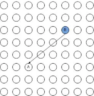
Third, we will discuss the time synchronization for long-distance as following. Assume that we have a sensor network as the Fig. 22, where the node A is the reference node, the node 1-4 are the node in single-hop, the node 5 is the node in long-distance.

We can divide this procedure of the time synchronization into two steps. Step 1, the node A and the node 1-4 will finish time synchronization as we mention before. Step 2, the node A uses the directional antenna to finish time synchronization with the node 5 as below.

Fig. 23 Our method-Step 1 for Long-distance Time Synchronization

In Fig. 23, the node A transmits a packet to the node 5 after the node A finish time synchronization in single-hop. If the deployment density is large enough, there is a node that already finish the procedure of the time synchronization between the node A and the node 5. We can use this node to be the time server. The receive table is shown as below, when the node A transmits a reference packet to the node 5.

T

Node 3 T r₃

Node 5 T r₅

Table. 15 Multihop-Receive Table

Time Node

The node 3 will reply a packet to the node A with the information of when receiving the reference packet, because the node 3 did not has the directional antenna to communicate with the node 5 as the Fig. 24 shows below.

Fig. 24 Our method-Step 2 for Long-distance Time Synchronization

The node A will transmit the time information of the node 3 to the node 5, when the node A receives the packet from the node 3 as the Fig. 25 shows below.

Fig. 25 Our method-Step 3 for Long-distance Time Synchronization

the node 5 receives the packet from the node A as the Table. 16 below.

T

Node 5 Tr₃− Tr₅

Table. 16 Multihop-Time Difference Table

In order to achieve the purpose of time synchronization, we can estimate the time offset between the node 5 and the node 3 from the Table. 16.

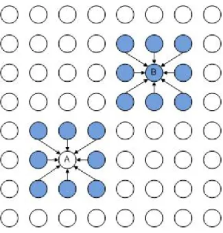
The node A uses the directional antenna to communicate with the node 5, after the node 5 finish the procedure of the time synchronization. The topology shows as below.

Fig. 26 Our method-Step 2 in Multihop

The gray nodes are the node that finished the procedure of time synchronization. Time

Next, we can use the nodes that already finish time synchronization to do the procedure of the time synchronization with others. For example, the Fig. 27 shows as below.

Fig. 27 Our method-Step 3 in Multihop

The node 5 as the node A do the procedure again as we describe before. The Fig. 28 shows as below, after the node 5 finishes the procedure of time synchronization.

The gray nodes are the node that finished the procedure of time synchronization. Next, we can use the node 6-10 to do the procedure of time synchronization with others. For example, the Fig. 29 shows as below.

Fig. 29 Our method-Step 5 in Multihop

The node 10 as the node A do the procedure again as we describe before. The Fig. 30 shows as below, after the node 10 finishes the procedure of time synchronization.

Fig. 30 Our method-Step 6 in Multihop

The gray nodes are the node that finished the procedure of the time synchronization. From these examples, we can clearly see that how to finish time synchronization from the node A starts the procedure of time synchronization to the node A uses the directional antenna to finish time synchronization with the node 5. Then, the node 5 uses the same way to finish time synchronization with others.

By the time synchronization scheme we proposed, we can find that we use the directional antenna to construct the shortcut in the small world. Let the time synchronization not just from the specific region to another, we use the directional antenna to extend the transmission range in the wireless sensor network. Therefore, the scheme we proposed greatly reduces the average path length between nodes, decreases the convergence time to finish the procedure of time synchronization.