Supplementary Article of ProteMiner-SSM

Supplementary Article of ProteMiner-SSM

Darby Tien-Hau Chang, Chien-Yu Chen+_{, Wen-Chin Chung, Yen-Jen Oyang}∗

Department of Computer Science and Information Engineering, National Taiwan University, Taipei, Taiwan, R.O.C.

Hsueh-Fen Juan Institute of Biotechnology and Department of Chemical Engineering

National Taipei University of Technology, Taipei, Taiwan, R.O.C. Hsuan-Cheng Huang

Institute of Biological Chemistry Academic Sinica, Taipei, Taiwan, R.O.C.

1. Illustration of the filtering process

The main distinction with respect to the software design of ProteMiner-SSM is the filtering process incorporated to expedite the analysis. The filtering process exploits the novel kernel density estimation algorithm that we have recently proposed [1, 2] to identify the crucial substructures on the contours of the protein tertiary structures that the analysis should focus on. In the design of ProteMiner-SSM, structural analysis is conducted at the residue level with each residue represented by its alpha carbon in the vector space. The efficient kernel density estimation algorithm treats the set of residues of a protein {s1, s2,…, sn} as n samples randomly taken from a probability

dis-tribution in the 3-dimensional vector space and employs the learning algorithm proposed in [1, 2] to construct an approximate probability density function of the following form:

) ( ˆ v f , 2 || || exp 1 1 2 2

∑

(i) v is a vector in an m-dimensional vector space,

(ii) β is the parameter that controls the smoothness of the approximation function, (iii) m m i i k R ) 1 ( ) 1 ( ) ( 2 + Γ + = =βδ β π σ si _and

R(si) is the k-th nearest neighbors of si,and k is a parameter to be set by the user. (iii)

∑

As the approximate probability density function presented in equation (1) is a continuous and smooth function in the vector space, we can expect that the function values at the residues located on the contour of the protein tertiary structure will generally be smaller than the function values at the inner residues. Accordingly, we can set

! _{This research is sponsored by National Science Council of R.O.C. under contract NSC 92-2323-B-002-013 and NSC 92-3112-B-027-001.} + _{This author is currently with Graduate School of Biotechnology and Bioinformatics, Yuan-Ze University, Chung-Li, Taiwan.}

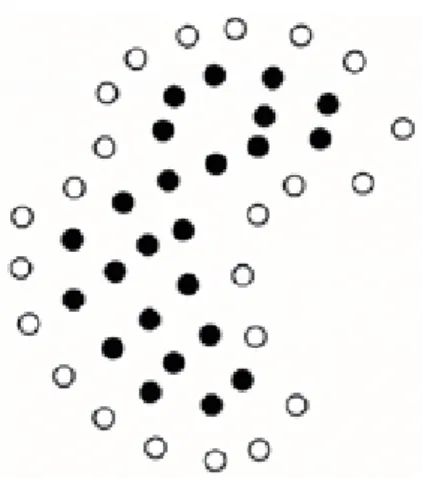
a threshold of the function values to distinguish those residues that are located on the contour of the protein terti-ary structure from those that are not. Fig. 1 depicts a 2-dimensional example to illustrate the effect of the filtering process. In this example, a 2-dimensional object is composed of a number of primitive instances represented by dots in the figure. Fig. 1(a) shows the instances that are identified as on the boundary of the object by the filtering process.

With the residues on the contour of the protein tertiary structure been successfully identified, the next task of the filtering process is to further classify each of these residues depending on whether it is located in a cave of the protein tertiary structure or not. This task can be carried out by applying equation (1) again but with a larger β value. Applying equation (1) with a larger β value implies that the approximate probability density function ob-tained is smoother. As a result, the function values at those residues that are located in a cave will be generally higher than the function values at those residues that are on the contour of the protein tertiary structure but not in a cave. Accordingly, a threshold can be set to classify these residues. Fig. 1(b) shows the final result obtained in this example and Fig. 2 shows the pseudo-code of the filtering process.

2. Time complexity of the filtering process

As far as the time complexity of the filtering process is concerned, in equation (1) we need to identify the k nearest neighbors for each of the n residues. If the kd-tree structure [3] is incorporated, then the average time complexity for constructing a kd-tree with n residues is O(n log n), provided that k is considered as a constant.

One practical implementation employed in this paper for evaluating equation (1) is to include only the nearest k’ residues of vector v, since the influence of the Gaussian function decreases exponentially. With this practice, the time complexity for evaluating the approximate function value at one residue is therefore O(k’ logn) and the

overall average time complexity of the filtering process is O(nlogn), if both k and k’ are considered as constants. Concerning the structural alignment process, as the geometric hashing algorithm narrows down its search space to only the coordinate systems defined by the residues located in the caves of the reference protein and the target protein, the time complexity for comparing the crucial substructures of these two proteins is O(n1′n2′(n1′+q)), where n′1 and n′2 are the numbers of residues identified as in the caves of the two proteins, respectively, and q is the number of residues in the binding sites of the reference protein.

3. Parameter settings

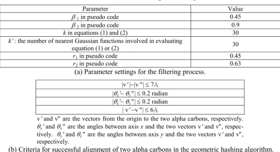
Table 1 shows how the parameters are set for the filtering process in our experiment and the criteria for successful alignment of two alpha carbons in the geometric hashing algorithm. One may wonder whether these parameters should be set differently, if different sets of proteins are to be analyzed. According to our experiences, when an-other reference protein is given, the only parameter values in Table 1(a) that need to be adjusted are r1 and r2. That is, except the values of r1 and r2, the user basically can adopt the parameter values listed in Table 1(a), when

parameter setting just represents a subjective tradeoff between the accuracy of the analysis and the magnitude of speedup obtained. By setting r1 to 1 and r2 to 0, we basically keep all the residues. On the other hand, by setting either r1 to 0 or r2 to 1, we can eliminate all the residues. Since we can realize our view of tradeoff without any limitation through adjusting the values of r1 and r2, there is no need to manipulate other parameters. Basically, when given a reference protein, the user needs to try a number of possible combinations of r1 and r2, and select one that can accurately extract the residues in the binding site of the reference protein.

The last issue that deserves further discussion is the magnitude of speedup due to the filtering process, which range from 3.11 to 9.79 times in our experiments. Since the expediting mechanism works by reducing the number of residues to be included in the analysis process, in principle, we could set the parameters listed in Table 1 with a conservative view and an insignificant magnitude of speedup would result. On the other hand, if we set the pa-rameters listed in Table 1 with a more aggressive view, then we could obtain a higher level of speedup but might lose some degree of analysis accuracy as a consequence.

4. Illustration of user interface

This section illustrates the user interface of ProteMiner-SSM with an experiment. In this experiment, the bio-chemist is given the crystal structure reported in [4], which consists of an integrin protein bound with a peptide ligand containing Arg-Gly-Asp, and wants to check whether some proteins in the caspase family contain a similar substructure as the binding site of integrin αVβ3. The biochemist therefore submitted a query to ProteMiner-SSM as demonstrated in Fig. 3(a). Fig. 3(b) shows the output generated by ProteMiner-ProteMiner-SSM. On the web page presented in Fig. 3(b), the user can click the protein that is of particular interest to examine the detailed mapping of the residues in the reference protein and in the target protein, as demonstrated in Fig. 3(c). It is typical that multiple possible alignments are found for each target protein and the user can examine these possible alignments with the 3-D viewer as demonstrated in Fig. 3(d).

References:

1. Oyang, Y.-J., Chang, D. T.-H., Chen, C.-Y., and Hwang, S.-C., Expediting Protein Structural Analysis with an Efficient Kernel Density Estimation Algorithm , In Proceedings of IEEE 5th International Symposium on Multimedia Software

Engineering, Taichung, Taiwan, 2003.

2. Oyang, Y.-J., Hwang, S-C, Ou, Y.-Y., Chen, C.-Y., and Chen, Z.-W. (2002) A Novel Learning Algorithm for Data Classification with Radial Basis Function Networks, In Proceedings of 9th International Conference on Neural

Infor-mation Processing (ICONIP-2002), Singapore, 2002.

3. Bentley, J. L. (1975) Multidimensional binary search trees used for associative searching, Communication of the ACM,

18, 509-517.

4. Xiong, J.P., Stehle, T., Zhang, R., Joachimiak, A., Frech, M., Goodman, S.L., and Arnaout, M.A. (2002) Crystal struc-ture of the extracellular segment of integrin alpha Vbeta3 in complex with an Arg-Gly-Asp ligand. Science. 296, 151-5

(a) The effect after the instances on the boundary of the object have been identified.

(b) The effect after the instances in the caves of the object have been identified.

Fig. 1. An example that illustrates the effects of the filtering process.

Algorithm kernel density estimation based filtering

Input: A set S = {s1, s2, …, sn} of instances in the vector space and parameters β1, β2, k, r1, and r2. Output: Sˆ , a subset of S.

Set Sˆ←S.

For each si ∈ S do the following:

Compute fˆ(s_i) according to equation (1) with β = β1.

Set max{ˆ( )} 1 i n f si w ≤ ≤ ← .

For each si ∈ S do the following: If fˆ(s_i)≥r₁⋅w, then Sˆ←Sˆ−{s_i}. For each si ∈ S do the following:

Compute fˆ(s_i) according to equation (1) with β = β2.

Set max{ˆ( )} 1 i n f si w ≤ ≤ ← .

For each si ∈ Sˆ do the following: If fˆ(s_i)≤r2⋅w, then Sˆ←Sˆ−{si}.

Instance identified as not on the bounary.

Instance identified as on the bound-ary.

Instance identified as not on the bounary.

Instance identified as on the bound-ary but not in a cave.

(a) Submission of a query to ProteMiner-SSM.

(b) Output page of ProteMiner-SSM.

(c) The detailed mapping of the residues in integrin (the reference protein) and in caspase-8 (the target protein).

Table 1. Parameter settings in the experiment.

Parameter Value

β 1 in pseudo code 0.45

β 2 in pseudo code 0.9

k in equations (1) and (2) 30

k′ : the number of nearest Gaussian functions involved in evaluating

equation (1) or (2) 30

r1 in pseudo code 0.45

r2 in pseudo code 0.63

(a) Parameter settings for the filtering process. |v′ |−|v ″| ≤ 7Å

|θx′− θx ″| ≤ 0.2 radian |θy′− θy ″| ≤ 0.2 radian

| v′ −v ″| ≤ 6Å

v′ and v″ are the vectors from the origin to the two alpha carbons, respectively. θx′ and θx ″ are the angles between axis x and the two vectors v′ and v″, respec-tively. θy′ and θy ″ are the angles between axis y and the two vectors v′ and v″, respectively.