OPTIMIZING MULTI-RESPONSE PROBLEMS IN THE
TAGUCHI METHOD BY FUZZY MULTIPLE ATTRIBUTE
DECISION MAKING
lee-ing tong and chao-ton suDepartment of Industrial Engineering and Management, National Chiao Tung University, 1001, Ta Hsueh Road, Hsinchu, Taiwan, R. O. C.
SUMMARY
One of the conventional approaches used in off-line quality control is the Taguchi method. However, most previous Taguchi method applications have only dealt with a single-response problem and the multi-response problem has received only limited attention. The theoretical analysis in this study reveals that Taguchi’s quadratic loss function and the indifference curve in the TOPSIS ( Technique for order preference by similarity to ideal solution) method have similar features. The Taguchi method deals with a one-dimensional problem and TOPSIS handles multi-dimensional problems. As a result, the relative closeness computed in TOPSIS can be used as a performance measurement index for optimizing multi-response problems in the Taguchi method. Next, an effective procedure is proposed by applying fuzzy set theory to multiple attribute decision making (MADM). The procedure can reduce the uncertainty for determining a weight of each response and it is a universal approach which can simultaneously deal with continuous and discrete data. Finally, the effectiveness of the proposed procedure is verified with an example of analysing a plasma enhanced chemical vapour deposition (PECVD ) process experiment. 1997 by John Wiley & Sons, Ltd.
key words: Taguchi method; parameter design; multi-response problem; multiple attribute decision making; TOPSIS method
1. INTRODUCTION design parameters and noise factors in the orthog-onal arrays. The signal-to-noise (SN) ratio is com-puted on the basis of quality loss for each experi-A cost-effective method to improve product quality
and operational procedures is with the use of off- mental combination. Finally, SN ratios are analysed to determine the optimal settings (i.e. control factors line quality control. This area includes those quality
control activities used in the product planning, and their levels) of the design parameters. The merits and shortcomings of the Taguchi method can design and production engineering stages ( but not
during actual production).1 The Taguchi method, be found in References 2, 4 and 5.2,4,5 However, a
customer usually considers more than one quality which combines the experimental design techniques
with quality loss considerations, is the conventional characteristic in most manufactured products. The Taguchi method can only be used for a single-approach used for off-line quality control. The
Tagu-chi method carefully considers the impact of the response case; it cannot be used to optimize a multi-response problem. Engineering judgement has, up various factors influencing performance variation.
This method consists of three stages: (a) systems until now, been used primarily for the optimization of the multi-response problem in the Taguchi design, (b) parameter design, and (c) tolerance
design. A more detailed description of these three method. Unfortunately, an engineer’s judgement will normally increase the uncertainty during the decision design types is provided by Kackar2 and Phadke.3
From their investigations, the variability and average making process. Another approach to solve such a problem entails the assigning of a weight for each of performance are of primary concern.
Product and operational procedures are influenced response. Determining a definite weight for each response in an actual case remains difficult. In by design parameters (i.e. factors that are controlled
by designers) and noise factors (i.e. factors that addition, a factor which is significant in a single response case is not necessarily significant when cannot be controlled by designers, such as
environ-mental factors). The parameter design of the Taguchi considered in a multi-response case. Therefore, a more effective approach is required to solve such a method involves selecting the levels of the design
parameters to minimize the effects of the noise complicated problem.
Fuzzy set theory provides membership functions factors. That is, the design parameter’s settings for
a product or a process should be determined so that which represent uncertain and subjective infor-mation. Multiple attribute decision making (MADM) the product’s response has the minimum variation,
and its mean is close to the desired target. Experi- refers to a situation in which selections among some courses of action must be made in the presence of mental design is used in this method to arrange the
CCC 0748–8017/97/010025–10 Received 5 October 1995
multiple, usually conflicting, attributes. In this paper, application could be limited. Their method increases the computational process complexity, thereby mak-a systemmak-atic procedure is developed vimak-a the mak-
appli-cation of fuzzy set theory to MADM to optimize ing it difficult for use on the shop floor. Vining and Myers9
applied the dual response approach to achi-the multi-response production process. A fuzzy
num-ber is first applied to determine the weight for each eve some of the goals of the Taguchi philosophy, specifically to obtain a target condition on the mean response. By considering the quality loss of each
response, a multi-response performance measure- while minimizing the variance. They focused on the single-response problem. Castillo and Montgomery10
ment index is developed on the basis of an MADM
method; namely, a technique for order preference by further showed that the generalized reduced gradient (GRG) algorithm can lead to better solutions than similarity to ideal solution ( TOPSIS). The developed
index can be used to determine the optimum con- those obtained with the dual response approach. They also demonstrated that the GRG algorithm can ditions in the parameter design stage for
multi-response problems. The proposed optimization pro- be applied to a multiple response problem. However, the above three methods may be difficult for those cedure includes a series of steps capable of
decreas-ing the uncertainty in engineerdecreas-ing judgement when users having limited statistical training. Phadke3
used the Taguchi method to study the the Taguchi method is applied. Only the static
qual-ity characteristic problem, in which the desired surface defects and wafer thickness in the polysil-icon deposition process for a VLSI circuit manufac-response value is fixed, is discussed in this paper.
The remainder of this paper is organized as fol- turer. Based on the judgement of relevant experience and engineering knowledge, trade-offs were made lows. A literature review of the multi-response
prob-lems in the Taguchi method is given in Section 2. in Phadke’s investigation to select the optimum factor levels for a problem with multiple quality Section 3 introduces MADM problems. Section 4
proposes an optimization procedure for solving the characteristics. By human judgement, the validity of the experimental results cannot be easily assured. problem of multi-response cases in the Taguchi
method. An illustrative example for the implemen- Contradictory results could be reached by different engineers addressing the problem. Therefore, the tation of the proposed procedure is provided in
Section 5. Concluding remarks are made in uncertainty in the optimum factor levels is increased. Phadke’s approach can usually only be used by an Section 6.
experienced engineer.
Hung11 transformed various types of quality
2. LITERATURE REVIEW
characteristics (smaller-the-better, larger-the-better and nominal-the-best) into the nominal-the-best Derringer and Suich6 demonstrated how several
response variables can be transformed into a desir- characteristics with a target of 0 and gave a weight to each quality characteristic for computing the SN ability function, which can be optimized by
univari-ate techniques. The desirability function approach is ratio. However, his method could not handle a prob-lem involving continuous and discrete data. When simple and permits the user to make subjective
judgements on the importance of each response. the weight of a particular quality characteristic is increased, the optimum conditions will not move However, the inexperienced user in assessing a
desirability value may lead to inaccurate results. toward the same direction of that quality character-istic; therefore, this result is unsatisfactory.
Khuri and Conlon7 proposed a procedure capable of
simultaneously optimizing several response variables Shiau12 assigned a weight to each SN ratio of the
quality characteristic and summed the weighted SN that can be represented by polynomial regression
models. They used a distance function to measure ratios for computing the performance measurement of a multi-response problem. For example, there are the deviation from the ideal optimum. By
minimiz-ing this function, one can specify suitable operatminimiz-ing two quality characteristics with SN ratios: SN1 =
−10logL1 and SN2 = −10logL2, where L1 and L2
conditions for the simultaneous optimization of the
responses. The notion of using the minimax represent the quality losses of these two character-istics. As a result, the weighted SN ratio for this approach in their method is quite similar to that
in the TOPSIS method. However, their method is two-response problem will be SN0 = w1(SN1) +
w2(SN2), where wiis the weight of the ith response. computationally complicated, thereby making it
dif-ficult to explain to practitioners. If SN0 = −10logL, where L can be viewed as the
total quality loss, we then have L = Lw1
1 · Lw22. This
Only limited attention has been given to
multi-response problems in the Taguchi method. Logo- equation is difficult to explain from the perspective of the Taguchi method’s quality loss.
thetis and Haigh8 applied the multiple regression
technique and the linear programming approach to Tai, Chen and Wu13claimed that quadratic
model-ling was invalid for non-symmetric loss functions. optimize a five-response process by the Taguchi
method. However, sufficient details were not pro- In their investigation, empirical loss functions were developed for a multi-response problem involving vided in their work to establish their procedure.
Moreover, if the t-values of the regression coef- six variables and nine responses for the surface mount process. Multiple responses can be converted ficients are insignificant or the value of R2
(the
loss of each response. However, these empirical loss salient features of the information. According to their taxonomy, TOPSIS, in which the information functions can only be used in a particular process.
When their method is applied, the empirical loss given is a cardinal preference of the attributes, is the most suitable technique for this study. A detailed functions need to be determined in advance.
Conse-quently, the complexity of the problem is increased description of this method is provided later in this paper.
if this does not occur.
Pignatiello14 presented a quadratic loss function
for multiple-response quality engineering problems. 3.2. Fuzzy multiple attribute decision making The expected loss function was expressed in terms
The classical MADM methods cannot effectively of a variance component and a squared
deviation-cope with uncertain (or imprecise) information. The from-target component. To minimize the expected
use of the fuzzy set theory is a perfect means to loss function, a predictive regression model
resolve such a difficulty. Fuzzy MADM methods ( univariate response ) can be established by using
are designed to solve MADM problems with fuzzy controllable variables. The repeated procedure was
data. A good source of existing fuzzy decision applied to minimize the expected loss by following
making studies can be found in the work of Zimmer-the descent direction and establishing a new local
mann.17
The existing fuzzy MADM approaches have experimentation region. One disadvantage of his
two major drawbacks. First, cumbersome compu-method is that the cost matrix is difficult to
deter-tations are required, thereby limiting fuzzy MADM’s mine, thereby making it nearly impossible to
esti-applicability to real world problems. Secondly, most mate the predictive regression model precisely.
approaches require that the problem’s data be Another limitation is that additional experimental
presented in a fuzzy format, even though they are observations are required in conparison to the
tra-crisp in nature. Converting tra-crisp data into a fuzzy ditional Taguchi method. Several different strategies
format will increase computational efforts. Accord-were also discussed in Pignatiello’s work. However,
ingly, Chen and Hwang18 proposed an approach
these strategies were either impractical or infeasible
to overcome these difficulties. Their approach is for determining the optimal factor/level combination.
composed of two major phases. The first phase Tong, Su and Wang15
proposed a procedure to
converts fuzzy data into crisp scores. When the determine the multi-response signal-to-noise
problem encountered contains only crisp data, classi-( MRSN) ratio through the integration of the quality
cal MADM methods can be used to determine the loss for all responses with the application of
Tagu-ranking order of alternatives in the second phase. chi’s SN ratios. In their method, it was still difficult
The procedure described in Section 4 is proposed to determine the weight ratio for responses. In
on the basis of Chen and Hwang’s approach to addition, the quality loss at each trial was divided
solving fuzzy MADM problems. by the maximum quality loss in the total of the
trials. In this case, it is likely that the optimal
factor/level combination could be dominated by the 3.3. TOPSIS ‘maximum quality loss’. This fact is not desired.
TOPSIS considers that the chosen alternative Accordingly, a more effective procedure is proposed
should have the shortest distance from the ideal in this work to optimize multi-response problems in
solution and the longest distance from the negative-the Taguchi method.
ideal solution. Such an approach is both comprehen-sible and functional. This approach stipulates only 3. MULTIPLE ATTRIBUTE DECISION that the attributes must be numerical and
compara-MAKING ble. For example, let a MADM problem be
expressed in matrix format as 3.1. Multiple attribute decision making
x1 x2 % xn
Multiple attribute decision making (MADM) involves the selection among some alternatives each having multiple, usually conflicting, attributes. From
D= A1 A2 : Am xx11 x12 % x1n 21 x22 % x2n : : : xm1 xm2 xmn (1) a practical viewpoint, the number of alternatives is
predetermined in the MADM problems. The term ‘attributes’ is referred to as a ‘goal’ or a ‘criterion’.
MADM problems have common characteristics. For where Ai(i =1, 2, %, m ) are possible alternatives; xj instance, multiple attributes usually conflict with (j =1, 2, %, n) are attributes with which alternative each other. Each attribute has a different measure- performances are measured; xij is the performance ment unit. The relative importance of each attribute of alternative Ai with respect to attribute xj. The is usually given by a set of weights. Many MADM procedure of TOPSIS can be described in the follow-methods are available, with each one having its own ing six steps.16
characteristics and applicability. Hwang and Yoon16
classified MADM problems on the basis of the type Step 1. Calculate the normalized decision matrix, R = [rij]m×n:
3.4. A comparison of Taguchi’s loss function and rij= xij
!
O
m i=1 x2 ij, i=1, 2, %, m; j=1, 2, %, n the indifference curve in TOPSIS
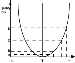
Taguchi’s quadratic loss function is presented in Figure 1, where y is the quality characteristic of a ( 2)
product and T is the target value for y. Notably, at y = T, the loss is zero. The loss increases slowly Step 2. Calculate the weighted normalized decision
when y is near T; however, the loss increases rapidly matrix, V = [vij]m×n:
as y goes further away from T. In Figure 1, the loss increases by AB when y is increased 1 unit vij=wjrij, i=1, 2, %, m; j=1, 2, %, n ( 3)
nearing T. The loss increases by CD when y is increased 1 unit further away from T. Obviously, where wj is the weight of the jth attribute and
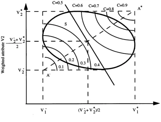
CD . AB. When the TOPSIS method is applied, some typical indifference curves for a two attributes
O
n j=1wj=1. problem are drawn and are presented in Figure 2.
In Figure 2, when C*
i $ 0·5 or is near 1 (close to the ideal solution A*), the marginal rate of
substi-Step 3. Determine the ideal and negative-ideal sol- tution decreases with an increase in V1. On the other
utions: hand, when C*
i , 0·5 or goes further from 1 (away from the ideal solution A*), the marginal rate of (a) The ideal solution:
substitution increases with an increase in V1. From
equation (8), we have cS*
i −( 1−c)S−i =0, where 0
A*={(max viju j P J),
, c , 1. This equation implies that the indifference (min viju j P J′)ui=1, 2, %, m}
curves observed in TOPSIS can be viewed as hyper-bolae. Taguchi’s quadratic loss function and the
={V*
1, V*2, %, V*j, %, V*n}, ( 4)
indifference curve in TOPSIS have similar features. (b) The negative-ideal solution: The latter can be viewed as an extension of the former. Notably, Taguchi deals with one-dimen-A−={( min viju j P J),
sional problems, in contrast, TOPSIS handles multi-(Max viju j P J′)ui=1, 2, %, m} dimensional problems. As a result, the relative close-ness computed in TOPSIS can be used as a
perform-={V−1, V−2, %, V−j, %, V−n}, ( 5)
ance measurement index for optimizing multi-response problems in the Taguchi method.
where J = { j = 1, 2, %, nu j associated with benefit criteria}; J′ = { j = 1, 2, %, nu j associated with
cost criteria}. 4. PROPOSED OPTIMIZATION PROCEDURE
The most frequent issues encountered in multi-Step 4. Calculate the separation measures: The
sep-response problems are ( a) the conflict among aration of each alternative from the ideal one is
responses, (b) a different measurement unit for each given as
response, and (c) a difficulty in assigning a set of weights to the present information regarding the relative importance of each response. To solve these S*
i =
!
O
nj=1
(vij−V*j)2, i=1, 2, %, m ( 6) issues, a systematic optimization procedure is pro-posed in this section of the paper. The propro-posed The separation of each alternative from the
nega-tive-ideal solution is given as
S−i =
!
O
nj=1
(Vij−V−j)2, i=1, 2, %, m ( 7)
Step 5. Calculate the relative closeness to the ideal solution: The relative closeness of Ai with respect to A* is defined as C* i = S−i S* i + S−i , i=1, 2, %, m ( 8)
Step 6. Rank the preference order: The alternative
Figure 1. Taguchi’s quadratic loss function
Figure 2. Typical indifference curves observed in TOPSIS10
procedure assumes that decision data are fuzzy. (b) Normalize these crisp scores in order to obtain a set of weights to represent the rela-That is, the relative importance of each response is
fuzzified in order to incorporate unquantifiable tive importance of each response such that and/or imperfect information into a decision. In
order to reduce the computational complexity and
O
nj=1
wj=1 to satisfy the perspective of Taguchi’s quality loss,
TOPSIS is applied to find a performance
measure-ment index for each trial. This index is calculated where w
j is the weight of the jth response ( j from the relative closeness as obtained from equ- = 1, 2, %, n).
ation (8). This index is referred to here as a
‘TOP-For example, the linguistic terms suggested by SIS’ value. The larger the TOPSIS value the better
Chen and Hwang18 are summarized in Table I. This
the product quality is implied. As a result, the
scale system is both comprehensible and feasible traditional Taguchi method can be applied on the
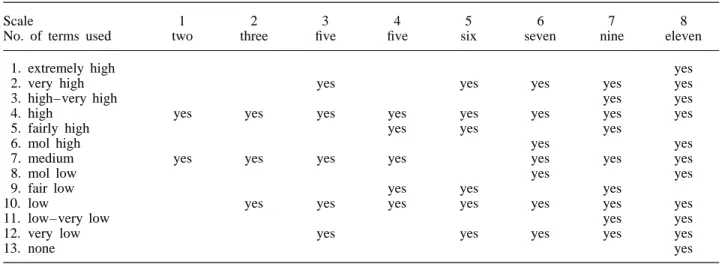
for practical applications. Table I is capable of basis of TOPSIS values. The proposed optimization
converting linguistic terms into fuzzy numbers. By procedure is described as follows in six detailed
applying Chen and Hwang’s fuzzy ranking method steps:
(using left and right scores), the crisp scores of fuzzy numbers in Table I are computed in Table II. Step 1. Transform the relative importance of each
The relative importance of three responses is response into a fuzzy number
assumed here to be very high, medium and low. (a) Express the relative importance of each Scales 3, 6, 7 and 8 in Table I contain these three response by the linguistic term, as determined terms. The simplest scale—scale 3—is chosen as from the experience of an engineer. our conversion scale. The corresponding crisp scores (b) Establish a formal scale system which can for these three responses can be found in Table II. be used to convert linguistic terms into their They are: 0·909 (very high), 0·500 (medium) and corresponding fuzzy numbers. 0·283 ( low). These three scores can be normalized (c) Find a conversion scale which matches all of by a simple calculation. For instance, for the first the linguistic terms. If more than one scale response ( very high), the normalized weight can be is found, the scale with the least number 0·537 = 0·909/( 0·909 + 0·500 + 0·283). The nor-of terms (the simplest scale) is to be used malized weights for the other two responses are
for conversions. 0·296 and 0·167.
Step 2. Assign crisp scores to the selected
Step 3. Compute the quality loss conversion scale ( fuzzy number)
(a) Apply a fuzzy scoring method to convert In this step, the quality loss for each response is computed. Notably, the quality loss computation for fuzzy numbers into crisp scores.
Table I. Linguistic terms used in the study
Scale 1 2 3 4 5 6 7 8
No. of terms used two three five five six seven nine eleven
1. extremely high yes
2. very high yes yes yes yes yes
3. high–very high yes yes
4. high yes yes yes yes yes yes yes yes
5. fairly high yes yes yes
6. mol high yes yes
7. medium yes yes yes yes yes yes yes
8. mol low yes yes
9. fair low yes yes yes
10. low yes yes yes yes yes yes yes
11. low–very low yes yes
12. very low yes yes yes yes yes
13. none yes
Table II. Crisp scores of fuzzy numbers
Scale 1 2 3 4 5 6 7 8
No. of terms used two three five five six seven nine eleven
1. extremely high 0·954 2. very high 0·909 0·917 0·909 0·917 0·864 3. high–very high 0·875 0·701 4. high 0·750 0·833 0·717 0·885 0·750 0·773 0·750 0·667 5. fairly high 0·700 0·584 0·630 6. mol high 0·637 0·590 7. medium 0·583 0·500 0·500 0·500 0·500 0·500 0·500 8. mol low 0·363 0·410 9. fair low 0·300 0·416 0·370 10. low 0·166 0·283 0·115 0·250 0·227 0·250 0·333 11. very–very low 0·125 0·299 12. very low 0·091 0·083 0·091 0·083 0·136 13. none 0·046
the ‘nominal-the-best’ response is based on the loss
y¯ij= 1 r
O
r k=1 yijk after adjusting the mean on target. According tothe Taguchi method, the following three formulae are given: s2 ij= 1 r−1
O
r k=1 (yijk−y¯ij) 2 Lij=k1 1 rO
r k=1 y2 ijk (9)k1, k2, k3 are quality loss coefficients, i = 1, 2, %,
m; j = 1, 2, %, n; k = 1, 2, %, r. for the smaller-the-better response
Step 4. Determine the TOPSIS value for each trial (a) Let Lij=k2 1 r
O
r k=1 1 y2 ijk (10) rij= Lij!
O
m i=1 L2 ij ( 12) for the larger-the-better responseand Lij=k3
S
sij y¯ijD
2 (11) vij=wjrij, i=1, 2, %, m; j=1, 2, %, n, ( 13) for the nominal-the-best response where wj is the weight of the jth responseobtained from step 2.
(b) Apply equations (4)–(8) to compute the rela-where Lij is the quality loss for the jth response at
the ith trial, yijk is the observed data for the jth tive closeness of each trial (C*i).
(c) The TOPSIS value in the ith trial is set to response at the ith trial, kth repetition, r is the
number of replications for each response, C*
Step 5. Determine the optimal factor/level tors were selected for optimization. These factors and their alternative levels are listed in Table III. combination
The standard array L18 was selected for the
experi-(a) Estimate the factor effects based on the
ment. The data for eighteen experiments are summa-TOPSIS value.
rized in Table IV. (b) Determine the optimal control factors and
their levels.
5.1. The conventional Taguchi approach
The difficulties encountered in optimizing multi-Step 6. Conduct the confirmation experiment
response problems are illustrated in the conventional A confirmation experiment should be performed
analysis based on the Taguchi method. The factor to verify that the optimum condition derived by the
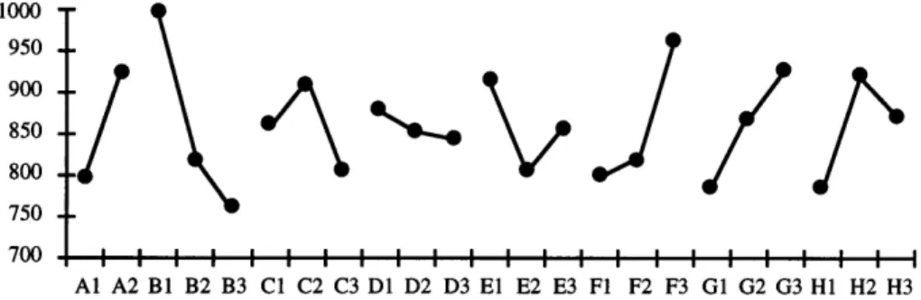
effects on SN ratios are illustrated in Figure 3. experiment actually yields an improvement. If the
According to the Taguchi method, the larger the SN predicted and observed SN ratios for each response
ratio, the better the quality. Therefore, the tentative are close to each other, one can conclude that the
optimum setting can be separately made in the fol-additive model on which the experiment was based
lowing: is a good approximation. As a result, the
rec-ommended optimum condition can be adopted for
RI response: A1B3C2D1E3F1G1H3 ( 14)
the process under study. If the predicted and
DT response: A1B1C3D2E2F2G2H3 ( 15)
observed SN ratios for one of the responses do not match, one may suspect that the additive model is
inadequate and that the interactions are important. Based on this observation, these two responses can In the latter case, another experiment may be neces- be optimized by setting factor A at level 1 and sary to achieve the required objective. setting factor H at level 3. However, determining the optimal settings for factors B, C, D, E, F and G can be complicated. For instance, factor B set at 5. IMPLEMENTATION level 3 creates an advantage for the RI response, but a disadvantage for the DT response. In contrast, A case study is presented in this section which
factor B set at level 1 creates an advantage for the verifies the effectiveness of the proposed
optimiz-DT response, but a disadvantage for the RI response. ation procedure. This case study involves the
This observation illustrates that different levels of improvement of a plasma enhanced chemical vapour
the same factor can be optimum for different deposition (PECVD) process in the fabrication of
responses. As a result, the decision is not clear. ICs. This case study was conducted by the Industrial
Technology Research Institute located in Taiwan. The three-inch wafers were mounted on holders
5.2. The proposed optimization procedure ( boats). Each boat can carry five wafers. The
depo-sition process entails depositing a uniform layer of When the proposed procedure was applied in this case study, the relative importances of responses silicon nitride (SiNx) with a specified thickness as
one step in the IC fabrication process. In the past, were first transformed into fuzzy numbers. From Table I, scales 1, 2, 3, 4, 6, 7 and 8 contain the uniformity of the output was unstable. The
reason for this low uniformity was unknown to the linguistic terms ‘high’ and ‘medium’. Scale 1 with the least number of terms is selected as the conver-process engineers. Therefore, these engineers were
unaware of how to adjust the multiple settings of sion scale. From Table II, the crisp scores for the two responses are: 0·750 (high) and 0·583 the process parameters when the quality of the wafer
was not meeting the requirements. In this study, an (medium). These two scores were then normalized and the normalized weights were 0·562 and 0·438 experiment was performed to determine the effects
of process parameters on the silicon nitride depo- which were obtained for the RI response and the DT response, respectively. Therefore, the TOPSIS sition process in order to raise the quality to meet
requirements. Optimal settings could hopefully be value for each trial could be determined by using equations (11), (12), (13) and equations (4) –(8). found in this experiment such that a high uniformity
( i.e. low variability) for the response can be achiev- The computational results are summarized in the last column of Table IV. The main effects on the ed.
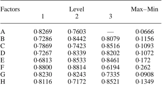
The two responses (in order of importance) are: TOPSIS values are summarized in Table V and their corresponding factor effects are plotted in Figure 4. ( a) RI: refractive index, in which the target value
is 2, and (b) DT: deposition thickness, in which the The controllable factors on a TOPSIS value in order of their significance are: F, E, H, B, C, D, G and target value is 1000 Å. The priority of the RI
response is higher than that of the DT response. A. The larger the TOPSIS value would imply the better the quality; consequently, the tentative optimal Following a discussion with the IC process
engin-eers, the relative importances of these two responses condition can be set as A1B2C3D2E2F2G2H3. The
predicted SN ratios under the optimum condition and are assumed to be ‘high’ and ‘medium’, respectively.
Table III. Control factors and their levels
Factor Level 1 Level 2 Level 3
A. Cleaning method No Yes —
B. The chamber temperature 100°C 200°C 300°C
C. Number of runs after the chamber has been cleaned 1st 2nd 3rd
D. The flow rate of SiH4 6% 7% 8%
E. The flow rate of N2 30% 35% 40%
F. The chamber pressure 160 mtorr 190 mtorr 220 mtorr
G. R. F. power 30 watt 35 watt 40 watt
H. Deposition time 11·5 min 12·5 min 13·5 min
*Starting levels are identified by underscore
Table IV. Data summary by experiment
Expt. Factors Deposition thickness (DT) Refractive index ( RI) Average TOPSIS
no. A B C D E F G H 1 2 3 4 5 1 2 3 4 5 DT RI value 1 1 1 1 1 1 1 1 1 694 839 728 688 704 2·118 1·919 1·985 2·085 2·056 730·6 2·033 0·8290 2 1 1 2 2 2 2 2 2 918 867 861 874 851 2·205 2·240 2·234 2·165 2·275 874·2 2·224 0·9718 3 1 1 3 3 3 3 3 3 936 954 930 1058 958 2·677 2·643 2·714 2·456 2·565 967·2 2·611 0·8423 4 1 2 1 1 2 2 3 3 765 828 842 768 801 2·096 1·997 1·949 2·046 2·000 800·8 2·018 0·9263 5 1 2 2 2 3 3 1 1 709 743 753 752 989 2·032 2·007 1·943 2·003 1·845 789·2 1·966 0·7686 6 1 2 3 3 1 1 2 2 795 785 846 722 833 1·860 1·838 1·842 1·999 1·858 796·2 1·879 0·8668 7 1 3 1 2 1 3 2 3 711 816 1085 787 1150 2·012 1·909 1·797 1·930 1·819 909·8 1·893 0·5820 8 1 3 2 3 2 1 3 1 580 644 602 607 811 1·834 1·760 1·760 1·782 1·744 648·8 1·776 0·8251 9 1 3 3 1 3 2 1 2 590 812 627 595 609 1·719 1·707 1·676 1·704 1·675 646·6 1·696 0·8302 10 2 1 1 3 3 2 2 1 917 1142 1126 916 966 2·097 1·911 1·889 2·014 1·960 1013·4 1·974 0·7851 11 2 1 2 1 1 3 3 2 1389 1405 1219 2063 1392 1·927 1·860 1·945 1·539 1·867 1293·6 1·828 0·6350 12 2 1 3 2 2 1 1 3 865 914 993 838 893 1·963 1·881 1·812 1·923 1·899 900·6 1·896 0·9086 13 2 2 1 2 3 1 3 2 827 884 884 851 1066 1·903 1·829 1·788 1·863 1·767 902·4 1·830 0·8706 14 2 2 2 3 1 2 1 3 787 805 780 776 976 2·103 2·020 2·011 2·107 1·968 824·8 2·042 0·8733 15 2 2 3 1 2 3 2 1 739 779 745 724 976 2·182 2·080 2·071 2·179 1·968 792·6 2·096 0·7598 16 2 3 1 3 2 3 1 2 724 721 690 1023 915 2·274 2·166 2·215 2·103 2·203 814·6 2·192 0·7284 17 2 3 2 1 3 1 2 3 771 806 785 869 859 1·942 1·905 1·909 1·916 1·900 818·0 1·914 0·9800 18 2 3 3 2 1 2 3 1 712 781 749 692 760 2·077 1·961 1·985 2·101 1·980 738·8 2·021 0·9017
Figure 3. (a ) Factor effects on SN ratios (RI response)
Figure 3. (b ) Factor effects on SN ratios (DT response)
limits for the prediction errors are computed and A2B1C2D2E2F2G2H2 are tabulated in Table VI.
According to the data in Table VI, an improvement presented in Table VI.
A confirmation experiment will verify the optimal in refractive index is 5·47 dB (the variance dropped to 32 per cent) and the deposition thickness is 9·89 condition. The results under the optimum condition
Table V. Main effects on TOPSIS values condition are not satisfactory, the flow rate of SiH4 can be increased and the R. F. power decreased.
Factors Level Max–Min This occurrence subsequently causes the RI response
1 2 3
to be close to its target value (2) and the DT response close to its target value (1000 Å).
A 0·8269 0·7603 — 0·0666
B 0·7286 0·8442 0·8079 0·1156
C 0·7869 0·7423 0·8516 0·1093 6. CONCLUSIONS
D 0·7267 0·8339 0·8202 0·1072
E 0·6813 0·8533 0·8461 0·172 Multi-response problems using the Taguchi method
F 0·8800 0·8814 0·6194 0·262 can be solved by assuming that the weight for each
G 0·8230 0·8243 0·7335 0·0908
response is known and that the weight is presented
H 0·8116 0·7172 0·8521 0·1349
by crisp numbers. However, it is difficult for the weight to be directly assigned by an engineer in most cases. Moreover, fuzzy set theory can be used effects on the averages of the RI response and the
DT response are plotted in Figures 5(a) and 5(b), to incorporate data which cannot be precisely assessed. In this study, a procedure involving the respectively. Factor D has only a slight effect on
the TOPSIS value and the average of the DT introduction of fuzzy data into a MADM problem has been proposed to achieve the optimization of response, but a more significant effect on the
aver-age of the RI response. Factor G has a slight effect multi-response problems in the Taguchi method. The procedure includes the following steps: (a) trans-on the TOPSIS value and the average of the RI
response, but a more significant effect on the aver- formation of the relative importance of each response, (b) assignment of crisp scores for the age of the DT response. Factors D and G can be
chosen as adjustment factors for RI response and selected conversion scale, (c) computation of the quality loss, ( d) determination of the TOPSIS value, DT response, respectively. For instance, if the
aver-ages of these two responses under the optimum (e) determination of the optimal factor/level
combi-Figure 4. Factor effects on TOPSIS values
Table VI. Results of confirmation experiment
Starting Optimum Optimum Improvement
condition condition condition
( prediction) (confirmation) Refractive index SN 32·09 32·29±5·94 37·56 5·47dB Average 2·0216 1·9074 Variance 0·00198 0·000638 Deposition thickness SN 22·58 27·99±6·57 32·47 9·89dB Average 1043·267 1039 Variance 6000·8 610·5
Figure 5. (b ) Factor effects on the average of the DT response
several response variables’, Journal of Quality Technology,
nation, and (f) performance analysis of a
confir-12, 214– 219 (1980).
mation experiment. Theoretical analysis in this study 7. A. I. Khuri and M. Conlon, ‘Simultaneous optimization
of multiple responses represented by polynomial regression
reveals that Taguchi’s quadratic loss function and
functions’, Technometrics, 23, 363–375 (1981).
the indifference curve in the TOPSIS method have
8. N. Logothetis and A. Haigh, ‘Characterizing and optimizing
similar features and are compatible. The Taguchi multi-response processes by the Taguchi method’, Quality and Reliability Engineering International, 4, 159– 169 (1988). method deals with a one-dimensional problem and
9. G. G. Vining and R. H. Myers, ‘Combining Taguchi and
TOPSIS handles a multi-dimensional problem. As a
response surface philosophies: a dual response approach’,
result, the relative closeness computed in TOPSIS Journal of Quality Technology, 22, 38–45 (1990).
10. E. Castillo and D. C. Montgomery, ‘A nonlinear
program-can be used as a performance measurement index for
ming solution to the dual response problem’, Journal of
optimizing multi-response problems in the Taguchi
Quality Technology, 25, 199– 204 (1993).
method. In the opinion of the authors, four signifi- 11. C. H. Hung, A cost-effective multi-response off-line quality
control for semiconductor manufacturing, Master thesis,
cant contributions are achieved in the proposed
pro-National Chiao Tung University, Taiwan, 1990.
cedure. First, the relative importance of each
12. G. H. Shiau, ‘A study of the sintering properties of iron
response can be expressed easily by the linguistic ores using the Taguchi’s parameter design’, Journal of the Chinese Statistical Association, 28 253– 275, (1990). term. Secondly, only one performance measurement
13. C. Y. Tai, T. S. Chen, and M. C. Wu, ‘An enhanced
( TOPSIS value) is required for the multiple
Taguchi method for optimizing SMT processes’, Journal of
responses at each experimental trial. Thirdly, the Electronics Manufacturing, 2, 91–100 (1992 ).
14. J. J. Pignatiello, Jr., ‘Strategies for robust multiresponse
procedure is a universal approach which can be
quality engineering’, IIE Transactions, 25, 5–15 (1993).
used in any type of multi-response problems.
15. L.-I. Tong, C.-T. Su and C.-H. Wang, ‘The optimization of
Fourthly, the proposed method can simultaneously multi-response problems in Taguchi method’, International Journal of Quality & Reliability Management, 14, (1997, deal with a multi-response problem involving both
forthcoming).
continuous and discrete data types. Additionally, an
16. C. L. Hwang and K. Yoon, Multiple Attribute Decision
experiment on the plasma enhanced chemical vapour Making—Methods and Applications, A State-of-the-Art Sur-vey, Springer-Verlag, New York, 1981.
deposition process in the IC manufacturing field has
17. H. J. Zimmermann, Fuzzy Set, Decision Making, and Expert
been performed to substantiate the authors’ proposed
System, Kluwer, Boston, 1987.
optimization procedure. 18. S. J. Chen and C. L. Hwang, Fuzzy Multiple Attribute Decision Making—Methods and Applications,
Springer-Ver-lag, New York, 1992.
acknowledgements
The authors would like to thank the National Science
Authors’ biographies:
Council of the R. O. C. for financial support of this manuscript under Contract No.
NSC-84–2121-M-009–022. The Industrial Technology Research Insti- Lee-Ing Tong is an associate professor in the Department tute (Taiwan) is also appreciated for assistance in of Industrial Engineering and Management at National Chiao Tung University, Taiwan, ROC. She received her accumulating the experimental data in this work.
B.S. from National Cheng Kung University, Taiwan, and M.S. and Ph.D. from University of Kentucky, USA, all in Statistics. She was an associate professor in the Depart-REFERENCES
ment of Mathematics at University of Massachusetts-Dartmouth, USA. Her current research activities include
1. G. Taguchi, E. A. Elsayed and T. Hsiang, Quality
Engineer-ing in Production Systems, McGraw-Hill Book Company, quality control, experimental design and Statistics in
indus-1989. trial applications.
2. R. N. Kackar, ‘Off-line quality control, parameter design and the Taguchi method (with discussion)’, Journal of Quality
Technology, 17, 176 –188 (1985). Chao-Ton Su is an associate professor in the Department
3. M. S. Phadke, Quality Engineering Using Robust Design, of Industrial Engineering and Management at National
Prentice-Hall, Englewood Cliffs, New Jersey, 1989. Chiao Tung University, Taiwan, ROC. He received his
4. G. E. P. Box, ‘Signal-to-noise ratios, performance criteria
B.S. and M.S. from Chung Yuan Christian University,
and transformation’, Technometrics, 30, 1– 17 (1988 ).
Taiwan, and Ph.D. from University of Missouri-Columbia,
5. N. Logothetis, ‘The role of data transformation in Taguchi
USA, all in Industrial Engineering. His current research
analysis’, Quality and Reliability Engineering International,
activities include quality engineering, production manage-4, 49– 61 (1988 ).