Protein metal binding residue prediction based on neural networks

(1)

PROTEIN METAL BINDING RESIDUE PREDICTION BASED

ON NEURAL NETWORKS

CHIN-TENG LIN

Brain Research Centre, University System of Taiwan; Department of Electrical and Control Engineering, National Chiao-Tung University, HsinChu, 300, Taiwan

[email protected] KEN-LI LIN

Department of Electrical and Control Engineering, National Chiao-Tung University,

Computer Center of Chung-Hua University, HsinChu, 300, Taiwan

[email protected] CHIH-HSIEN YANG

Institute of Bioinformatics, National Yang-Ming University, Taipei, 115, Taiwan

[email protected] I-FANG CHUNG

Institute of Bioinformatics, National Yang-Ming University, Taipei, 115, Taiwan

[email protected] CHUEN-DER HUANG Department of Electrical Engineering, HsiuPing Institute of Technology, Dali,

Taichung, 412, Taiwan [email protected]

YUH-SHYONG YANG

Brain Research Centre, University System of Taiwan; Institute of Bioinformatics, National Chiao-Tung University,

HsinChu, 300, Taiwan [email protected]

Over one-third of protein structures contain metal ions, which are the necessary elements in life systems. Traditionally, structural biologists were used to investigate properties of metalloproteins (pro-teins which bind with metal ions) by physical means and interpreting the function formation and reac-tion mechanism of enzyme by their structures and observareac-tions from experiments in vitro. Most of proteins have primary structures (amino acid sequence information) only; however, the 3-dimension structures are not always available. In this paper, a direct analysis method is proposed to predict the protein metal-binding amino acid residues from its sequence information only by neural net-works with sliding window-based feature extraction and biological feature encoding techniques. In four major bulk elements (Calcium, Potassium, Magnesium, and Sodium), the metal-binding residues are identiﬁed by the proposed method with higher than 90% sensitivity and very good accuracy under 5-fold cross validation. With such promising results, it can be extended and used as a powerful method-ology for metal-binding characterization from rapidly increasing protein sequences in the future. Keywords: Bioinformatics, life elements; metalloprotein; artiﬁcial neural networks (ANNs).

71

Int. J. Neur. Syst. 2005.15:71-84. Downloaded from www.worldscientific.com

(2)

1. Introduction

It is very interesting that more than one-quarter of the elements in periodic table are required for life,1 and most of them are metal ions. Many enzymes incorporate metal divalent cations and transition metal ions within their structures to stabilize the folded conformation of protein or to directly par-ticipate in the chemical reactions catalyzed by the enzyme.2 Metal also provides a template for protein folding, as in the zinc ﬁnger domain of nucleic acid binding proteins, the calcium ions of calmodulin (a protein molecule that is necessary for many biochem-ical process, including muscle contraction and the release of a chemical that carries nerve signals), and the zinc structural center of insulin. Besides, metal ions can also serve as redox centers for catalysis, such as heme-iron centers, copper ions and non-heme irons. Other metal ions can be used as electrophilic reactants in catalysis, as in the case of active site zinc ions of the metalloprotease (enzymes that catalyze the splitting of proteins into smaller peptide fractions and amino acids by a process known as proteolysis. In other words, these enzymes hydrolyze proteins).

In fact, the research of metalloprotein is involved in bioinorganic (or biological inorganic) chemistry which is the study of interactions between inorganic substances and molecules of biological interest, e.g., protein or DNA. Since metalloprotein participates in the most important biochemical processes, includ-ing respiration, nitrogen ﬁxation and oxygenic pho-tosynthesis, it is also one of main foci of bioinorganic chemistry. In addition, life originates and evolves from earth’s crust, an inorganic environment. This fact again emphasizes the importance of bioinorganic research, including metalloprotein.

Genome sequencing has “revolted” many ﬁelds in life science and bioinformatics is devoted to oﬀer rapid and accurate analysis in silico with these large amounts of biological data. In the beginning, most foci are on 2 major molecules in life: protein and DNA and many internet websites are designed for collecting their biological resources, e.g., Pro-tein Date Bank (http://www.rcsb.org/pdb/) and GenBank (http://www.ncbi.nlm.nih.gov/Genbank/ index.html).3,4 Recently, people start to notice the need for bioinorganic chemistry which was not received great attention in this postgenomic area.5,6 Therefore, building genomic and proteomic linkage on current basis of biological data becomes one of

the most important and urgent issue for extending bioinorganic related searches into genome-wide scale. Moreover, there is a wide range of computational tools required to effectively process and analyze such huge amount of biological data. Especially, various machine learning techniques including self-organized maps (SOM), artificial neural networks (ANNs), sup-port vector machine (SVM), and fuzzy logic have obtained great success in many fields in biological and medical researches, such as coding region recog-nition on DNA, protein structure prediction, and diagnosis of disease.7 In this paper, one simple data combination approach for metal ions and protein is illustrated in Sec. 2. In Sec. 3, an artificial neural network-based scheme is designed to identify bind-ing (interactbind-ing) residues with metal ions in protein molecules from protein sequences. The experimental results with 5-fold cross validation are presented in Sec. 4.

2. Materials: Dataset and Biological Resources

Before building the model of metal-binding residue prediction, one must identify all components in met-alloprotein and organize them into comprehensive way logically. Following the descending order by their physical size, there are 4 layers in hierarchical and abstract model of metalloprotein: protein, chain, site and ligand. The top level (see also Fig. 1) is protein which may contain one or more than one chains, and each chain is represented as one polypeptide chain belonging to one protein in nature. Each chain may be “inhabited” several sites on it. Every site contains the coordinate information about the entire metal center binding site as shown in the left corner of Fig. 1. One site is composed of molecules including amino acid or other non-amino acid complex sur-rounding the metal center. That is the second coordi-nation shell of central metal and in this paper, what we try to predict are the locations of these molecules (amino acid residues only) on the protein sequence. Furthermore, each atom directly interacting with the metal is called “ligand.” In the coordinate chemistry, it refers to atom or chemical group on the ﬁrst coordi-nation shell bound to the central atom which is usu-ally a metal via dative bond, which refers that one of the atoms gives up or yields electrons to another to form this bond. In biochemistry, it becomes more

(3)

Chain B Site 1 of Chain B Chain A Site 1 of Chain A Site 2 of Chain A Site 2 of Chain B Metal center One protein

One Site Binding residue or molecule Binding ligand (atom)

Fig. 1. Metal-binding protein structure model and hierarchy.

universal, i.e., any low molecule weight compound, including metal ion and metal compound bound to the other macromolecule. In this paper, the former deﬁnition is used.

The main data resources come from two web sites, one is the metalloprotein database and browser (MDB, the latest release is 18 and updated at Jan-uary, 17, 2003).8 of metalloprotein structure and design program of the Scripps Research Institute (http://metallo.scripps.edu) where all proteins with binding metal can be entirely extracted and the metal-binding site is also deﬁned by nearby amino acid residues and compounds via distance-dependent criteria. Another resource is Protein Data Bank (PDB) which provides general information about every protein structure. Hence, by combining these databases, the detail description of metalloprotein can be driven. For simplicity, the PDB infor-mation can be replaced by another compacted data — PDBFinder (http://www.cmbi.kun.nl/gv/ pdbﬁnder/).9

In integrated database, there are 19771 dis-tinct proteins and 7559 of them with metal-binding. Namely, over one-third (36.72%) of proteins are metalloproteins. Furthermore, there are 43 kinds

of element concerned in MDB. After cross refer-encing by PHP script language from local inte-grated MySQL database, 41 and 36 elements (it is because that some entries in MDB cannot find cor-responding protein sequence in PDBFinder) can be found in “protein set” and “enzyme set” respectively (Table 1). Protein set is defined by the collection of protein peptide chains binding to metal according to the records in MDB, and some of these chains belong to parts of enzyme which can catalyze chem-ical reactions. Hence, this special subset is identi-fied and isolated as another dataset named enzyme set. From metal-binding information of MDB and sequence information of PDBFinder, every amino acid residue in protein chain sequence can be marked as binding or non-binding and used as the training target afterward.

3. Method: Machine Learning Scheme Under the assumption that the behavior of metal-binding residue is inﬂuenced by the surrounding envi-ronment in nature, it is necessary to “observe” these protein sequences in wider scope than a single one amino acid so as to “decide” whether the metal-binding phenomena happen or not. Therefore, the prediction model under this assumption takes sub-sequences of protein as input materials and sets its output as “binding” or “non-binding.” Furthermore, each input vector applied to learning machine is one segment extracted from entire protein polypeptide chain by the concept — sliding window. Each slid-ing window is centered by the “target” amino acid. And the rest of the amino acids in window are the “neighbors” of this target residue. Figure 2 illustrates the model of sliding-window encoding and learning scheme when the window size is set as 5.

The learning scheme used in our experiments is Multi-Layer Perceptron (MLP) neural networks with back-propagation (BP) learning rule, where one hid-den layer with 30 hidhid-den nodes is used. Number of input nodes is dependent on the number of features used to represent one amino acid and the range of observation (size of window). In order to indicate the metal-binding or non-metal-biding state of tar-get amino acid residue, two output nodes are used. Binding state is represented by setting values of 2 output nodes as (1, 0) and the non-binding state is (0, 1) while training.

(4)

Table 1. List of elements in metal-binding residue prediction. The biological level of metal involves their concentration in living organism. The element type is the element classiﬁcation adapted from periodic table.

Biological level Name Element type Chains in protein set Chains in enzyme set Full name

Bulk element Ca Alkaline metal 2589 1106 Calcium

K Alkali metal 442 234 Potassium

Mg Alkaline metal 1999 863 Magnesium

Na Alkali metal 864 484 Sodium

Trace element Co Transition metal 192 110 Cobalt

Cr Transition metal 7 6 Chromium

Cu Transition metal 581 216 Copper

Fe Transition metal 2893 861 Iron

I Halogen 78 33 Iodine

Mn Transition metal 1003 434 Manganese

Mo Transition metal 128 70 Molybdenum

Ni Transition metal 208 101 Nickel

Se non-metal 225 110 Selenium

V Transition metal 26 12 Vanadium

Zn Transition metal 2433 1087 Zinc

Possibly essential trace As Semi-metal 111 64 Arsenic

element

N/A Ag Transition metal 3 1 Argentum, Silver

Al Basic metal 82 41 Aluminium

Au Transition metal 14 2 Gold

Ba Alkaline metal 3 2 Barium

Be Alkaline metal 24 3 Beryllium

Cd Transition metal 379 82 Cadmium

Cs Alkali metal 7 4 Cesium

Eu Rare Earth 2 1 Europium

Gd Rare Earth 16 0 Gadolinium

Hg Transition metal 236 117 Hydrargyrum,

Mercury

Ho Rare Earth 7 1 Holmium

In Basic metal 1 0 Indiana

La Rare Earth 5 0 Ianthanum

Li Alkali metal 3 2 Lithium

Pb Basic metal 31 16 Lead

Pt Transition metal 8 3 Platinum

Rb Alkali metal 1 0 Rubidium

Sm Rare Earth 20 3 Samarium

Sr Alkaline metal 13 3 Strontium

Tb Transition metal 1 0 Terbium

Te Semi-metal 4 2 Tellurium

Ti Basic metal 18 18 Thallium

U Transition metal 80 16 Uranium

W Transition metal 46 4 Tungsten

Yb Rare Earth 17 7 Ytterbium

In this paper, our experiments are divided into 3 subsections. First subsection is a preliminary test to compare non-biological coding and biological cod-ing. Two input coding methods are used (shown in Table 2) in the ﬁrst experiment. One is the direct

one-hot coding, which represents every amino acid as one 20-bit vector. Only one bit in the vector is ‘1’ and the other bits in the vector are ‘0’. In this way, every type of natural amino acid can be indi-cated by the position of the only “1” bit. Owing

(5)

Target residue

Raw amino acid sequence of one chain

Sliding Window (window size= 5) Feature vector Encoding Learning Machine Feed Left neighboring residues Right neighboring residues

…V L E N R A A Q G N G G…

Decide whether target residue (central position of window) is metal-binding or not

…V L E N R A A Q G N G G…

NEXT sliding window

Window sliding direction

NEXT Target residue

Fig. 2. Feature extraction, learning scheme and sliding window.

Table 2. Biological coding and one-hot coding for 20 amino acids. First column is one-letter code of amino acid. Sec-ond column is the occurrence probability and columns 3 to 5 are the propensities of secSec-ondary structure. Column 6 is metal-binding propensity (normalized frequency) and the last column is one-hot coding vector.

Amino acid Biological coding One-hot coding

Occurrence Helix Strands Trun Metal-binding propensity

A 7.49 1.41 0.72 0.82 0.032 100000000000000000000 C 1.82 0.66 1.40 0.54 0.658 010000000000000000000 D 5.22 0.99 0.39 1.24 1.000 001000000000000000000 E 6.26 1.59 0.52 1.01 0.659 000100000000000000000 F 3.91 1.16 1.33 0.59 0.035 000010000000000000000 G 7.10 0.43 0.58 1.77 0.120 000001000000000000000 H 2.23 1.05 0.80 0.81 0.967 000000100000000000000 I 5.45 1.09 1.67 0.47 0.040 000000010000000000000 K 5.82 1.23 0.69 1.07 0.033 000000001000000000000 L 9.06 1.34 1.22 0.57 0.043 000000000100000000000 M 2.27 1.30 1.14 0.52 0.063 000000000010000000000 N 4.53 0.76 0.48 1.34 0.198 000000000001000000000 P 5.12 0.34 0.31 1.32 0.017 000000000000100000000 Q 4.11 1.27 0.98 0.84 0.075 000000000000010000000 R 5.22 1.21 0.84 0.90 0.021 000000000000001000000 S 7.34 0.57 0.96 1.22 0.092 000000000000000100000 T 5.96 0.76 1.17 0.90 0.117 000000000000000010000 V 6.48 0.90 1.87 0.41 0.072 000000000000000001000 W 1.32 1.02 1.35 0.65 0.009 000000000000000000100 Y 3.25 0.74 1.45 0.76 0.081 000000000000000000010 X 0.00 0.00 0.00 0.00 0.000 000000000000000000001

(6)

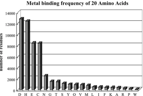
to the possible unknown type (usually using the symbol ‘X’ in sequence) of amino acid in a pro-tein sequence, one bit is added to record this con-dition. This is the so-called “non-biological” coding for amino acid. Another coding method is done by referencing 5 diﬀerent biological attributes of amino acid. They can be divided into 3 types: probabil-ity of occurrence from statistics of NCBI (National Center for Biotechnology Information, http://www. ncbi.nlm.nih.gov/) database adapted from amino acid properties of PROWL (a resource for protein chemistry and mass spectrometry developed in col-laboration of ProteoMetrics and Rockefeller Uni-versity http://prowl.rockefeller.edu/aainfo/contents. htm), propensities of three protein secondary struc-tures (helix, strand, and turn),10 and frequency of metal-binding from our integrated database as shown in Fig. 3.

In the second subsection of experiments, in order to study the effect of window size and realize whether the most “verbose” (comparing to biological coding of 5 attributes in the first experiment, the one-hot coding costs 21 bits) coding can bring better pre-diction results, prepre-diction models encoded by one-hot coding method with different size (from 5 to 17) of sliding window are used on sampled subset from enzyme set with mutually sequence identity (SID) below 25%, where SID is defined as the frac-tion of identical amino acids and the total length of sequence after multiple sequence alignment. By doing this, one can avoid the sequence homology bias while models are trained and tested, and it also

0 2000 4000 6000 8000 10000 12000 14000 number of residues D H E C N G T S Y Q V M L I F K A R P W

Amino Acid (One letter code)

Metal binding frequency of 20 Amino Acids

Fig. 3. Metal-binding frequency of 20 amino acids.

helps to retain the generalization ability of the pro-posed prediction model. That is, there are no huge amounts of similar sequences (sequence homology) dominating entire dataset and thus it will greatly influence the prediction models to fit them only. Before performing this experiment, we expect to see the performance becomes better with increase of win-dow size. However, it is not “economical” to expand the range of observation on primary structure of pro-tein (amino acid sequence of propro-tein) unlimitedly. In fact, whether it is practical or not to increase the window size while encoding protein sequence information fed to the prediction model is the most important issue need to be concerned. If it is indeed an effective way to achieve promising result at “rea-sonable” size of window, what is the optimal size for predicting metal-binding residues from protein sequences? If not, is there any better way to pro-mote previous model in the first experiment other than increasing the size of window?

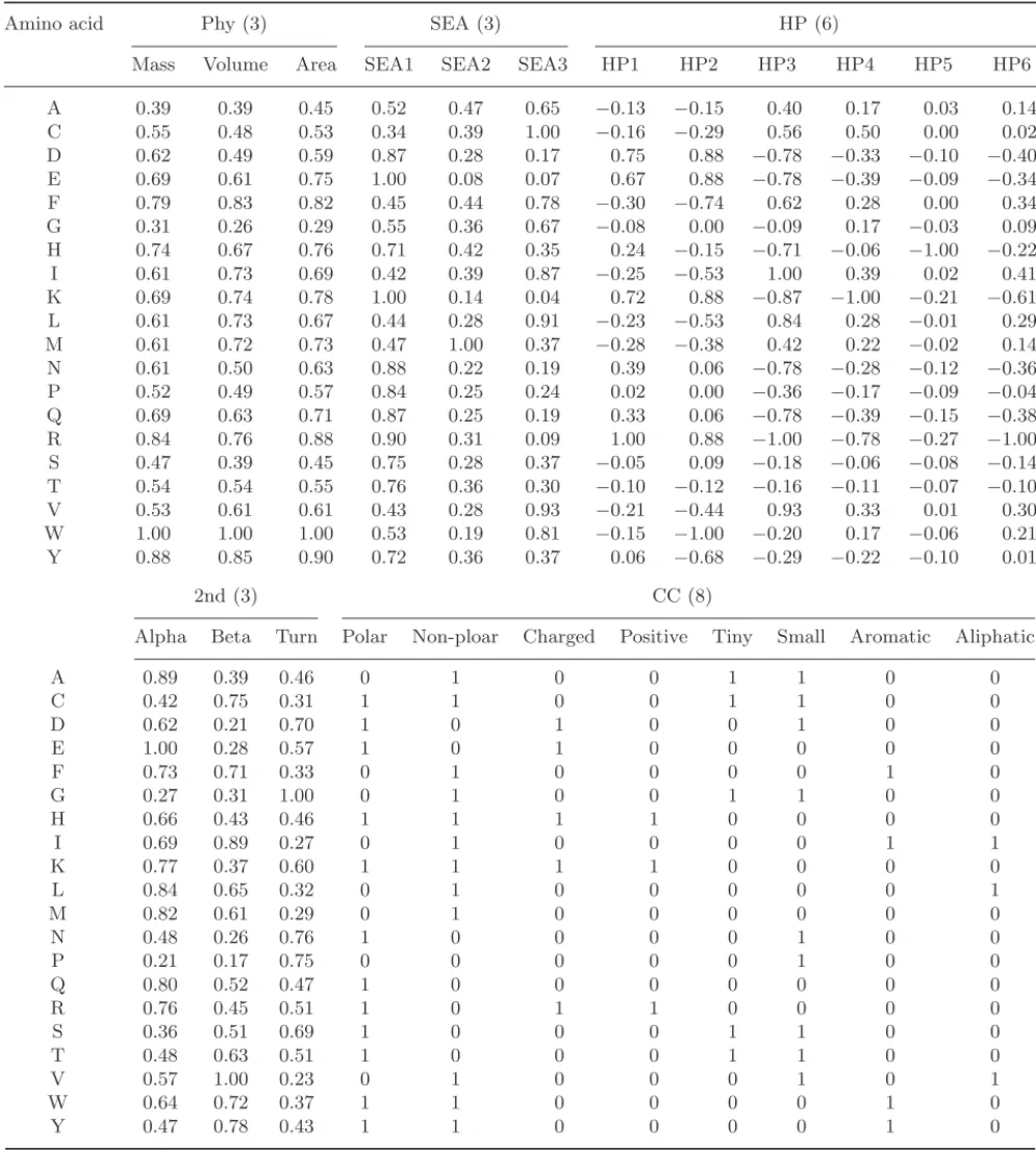
Finally, comparing to the second subsection which tries to optimize the model by adjusting the window size while using one-hot coding, the third subsection will introduce more biological feature “sets” and enhance the performance of model sub-stantially. In addition, there are only 5 attributes used in the first subsection and they are combined as one feature set of biological coding. Consequently, in this subsection more biological attributes will be used and organized more systematically. We add 5 different feature sets and their abbreviations are: Phy, SEA, HP, 2nd and CC. “Phy” contains 3 ele-mentary Physical measures (mass, volume and sur-face area) of amino acids. Further, “SEA” is the abbreviation of Solvent Exposed Area. SEA defines 3 attributes which refer to the possibility of amino acid to have exposed area in the solvent under 3 different conditions: SEA (solvent exposed area for short) greater than 30 angstrom2, SEA between 10 to 30 angstrom2and SEA less than 10 angstrom2. Every amino acid has its own possibility to have different size of SEA under this feature set. “HP” is referred to HydroPhobicity which states the degree of water-repellent of non-polar molecule (it refers to amino acid here) and there are 6 different HP scales from 6 different authors/groups contributed to HP fea-ture set. The term “2nd” is the abbreviation of sec-ondary structure of protein including helix, strand and turn as used as part of biological coding in the

(7)

Table 3. Deﬁnition and references of 5 biological feature sets.

Feature set name (size) Deﬁnition and content References

mass

Phy (3) Three physical measures of amino acid volume NCBI statistics area

Three levels solvent exposed area (SEA) of SEA> 30

SEA (3) amino acids with thershold 10 and 30 10< SEA < 30 (Ref. 12)

(angstrom square) SEA< 10

Engleman-Steitz (Ref. 13) Hoop-Woods (Ref. 14) HP (6) Hydrophobicity scales from six diﬀerent Kyte-Doolittle (Ref. 15)

authors Janin (Ref. 16)

Chothia (Ref. 17)

Eisenberg Weiss (Ref. 18) Alpha helix

2nd (3) Propensities of three secondary structures Beta strand (Ref. 10) Turn (loop, coil)

Polar Non-Polar

Charged

CC (8) Classiﬁcations of amino acids, it divides Positive (Ref. 11) 20 natural aminno acids into eight classes Tiny

Small Aromatic Aliphatic

first subsection. At last, CC is defined by Chemical Classification of 20 amino acids. It classifies these amino acids into 8 groups: polar, non-polar, charged, positive, tiny, small, aromatic and aliphatic. Because this classification is “overlapped” (namely, one amino acid may be assigned to more than one group), we define this feature set as 8-bit vector and each posi-tion corresponds to the group of classificaposi-tion in the order as previously mentioned. For example, while amino acid A is classified to non-polar (2nd group), tiny (5th group) and small (6th group), its feature under “CC” coding is “01001100.” More details and references of these feature sets are shown in Table 3 and their arithmetic values are listed in Table 4.

4. Experimental Results and Discussions

In the following experiments, there are two major data sets–protein set and enzyme set. Each type of element has its own neural network for prediction and 5-fold cross validation is used to evaluate the performance. There are 5 performance indexes

listed– accuracy (1), positive predictive rate (2), sen-sitivity (3), speciﬁcity (4) and negative predictive rate (5) which are calculated from true positive (TP), true negative (TN), false positive (FP), and false neg-ative (FN) values. These elementary measures of per-formance are deﬁned and shown in Table 5.

accuracy = TP + TN

TP + TN + FP + FN (1) positive predictive rate = TP

TP + FP (2)

sensitivity = TP

TP + FN (3)

speciﬁcity = TN

TN + FP (4)

negative preditive rate = TN

TN + FP (5)

4.1. Comparisons between non-biological coding and biological coding

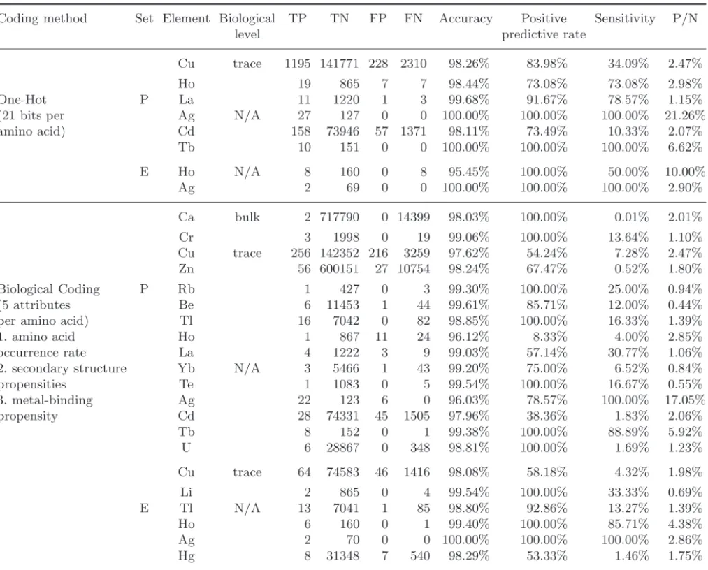
Table 6 lists the metal-dependent subset with non-zero TP by applying 2 coding methods (one-hot coding and biological coding) in both protein set

(8)

Table 4. Values of 5 biological feature sets (Phy, SEA, HP, 2nd and CC).

Amino acid Phy (3) SEA (3) HP (6)

Mass Volume Area SEA1 SEA2 SEA3 HP1 HP2 HP3 HP4 HP5 HP6

A 0.39 0.39 0.45 0.52 0.47 0.65 −0.13 −0.15 0.40 0.17 0.03 0.14 C 0.55 0.48 0.53 0.34 0.39 1.00 −0.16 −0.29 0.56 0.50 0.00 0.02 D 0.62 0.49 0.59 0.87 0.28 0.17 0.75 0.88 −0.78 −0.33 −0.10 −0.40 E 0.69 0.61 0.75 1.00 0.08 0.07 0.67 0.88 −0.78 −0.39 −0.09 −0.34 F 0.79 0.83 0.82 0.45 0.44 0.78 −0.30 −0.74 0.62 0.28 0.00 0.34 G 0.31 0.26 0.29 0.55 0.36 0.67 −0.08 0.00 −0.09 0.17 −0.03 0.09 H 0.74 0.67 0.76 0.71 0.42 0.35 0.24 −0.15 −0.71 −0.06 −1.00 −0.22 I 0.61 0.73 0.69 0.42 0.39 0.87 −0.25 −0.53 1.00 0.39 0.02 0.41 K 0.69 0.74 0.78 1.00 0.14 0.04 0.72 0.88 −0.87 −1.00 −0.21 −0.61 L 0.61 0.73 0.67 0.44 0.28 0.91 −0.23 −0.53 0.84 0.28 −0.01 0.29 M 0.61 0.72 0.73 0.47 1.00 0.37 −0.28 −0.38 0.42 0.22 −0.02 0.14 N 0.61 0.50 0.63 0.88 0.22 0.19 0.39 0.06 −0.78 −0.28 −0.12 −0.36 P 0.52 0.49 0.57 0.84 0.25 0.24 0.02 0.00 −0.36 −0.17 −0.09 −0.04 Q 0.69 0.63 0.71 0.87 0.25 0.19 0.33 0.06 −0.78 −0.39 −0.15 −0.38 R 0.84 0.76 0.88 0.90 0.31 0.09 1.00 0.88 −1.00 −0.78 −0.27 −1.00 S 0.47 0.39 0.45 0.75 0.28 0.37 −0.05 0.09 −0.18 −0.06 −0.08 −0.14 T 0.54 0.54 0.55 0.76 0.36 0.30 −0.10 −0.12 −0.16 −0.11 −0.07 −0.10 V 0.53 0.61 0.61 0.43 0.28 0.93 −0.21 −0.44 0.93 0.33 0.01 0.30 W 1.00 1.00 1.00 0.53 0.19 0.81 −0.15 −1.00 −0.20 0.17 −0.06 0.21 Y 0.88 0.85 0.90 0.72 0.36 0.37 0.06 −0.68 −0.29 −0.22 −0.10 0.01 2nd (3) CC (8)

Alpha Beta Turn Polar Non-ploar Charged Positive Tiny Small Aromatic Aliphatic

A 0.89 0.39 0.46 0 1 0 0 1 1 0 0 C 0.42 0.75 0.31 1 1 0 0 1 1 0 0 D 0.62 0.21 0.70 1 0 1 0 0 1 0 0 E 1.00 0.28 0.57 1 0 1 0 0 0 0 0 F 0.73 0.71 0.33 0 1 0 0 0 0 1 0 G 0.27 0.31 1.00 0 1 0 0 1 1 0 0 H 0.66 0.43 0.46 1 1 1 1 0 0 0 0 I 0.69 0.89 0.27 0 1 0 0 0 0 1 1 K 0.77 0.37 0.60 1 1 1 1 0 0 0 0 L 0.84 0.65 0.32 0 1 0 0 0 0 0 1 M 0.82 0.61 0.29 0 1 0 0 0 0 0 0 N 0.48 0.26 0.76 1 0 0 0 0 1 0 0 P 0.21 0.17 0.75 0 0 0 0 0 1 0 0 Q 0.80 0.52 0.47 1 0 0 0 0 0 0 0 R 0.76 0.45 0.51 1 0 1 1 0 0 0 0 S 0.36 0.51 0.69 1 0 0 0 1 1 0 0 T 0.48 0.63 0.51 1 0 0 0 1 1 0 0 V 0.57 1.00 0.23 0 1 0 0 0 1 0 1 W 0.64 0.72 0.37 1 1 0 0 0 0 1 0 Y 0.47 0.78 0.43 1 1 0 0 0 0 1 0

and enzyme set (without sequence similarity sam-pling) after 5-fold cross validation. In the ﬁrst col-umn, coding methods are summarized and in the second column “set”, P and E represent Protein set and Enzyme set, respectively. There are several

observations as follows. First, the neural network can detect more types of life elements in protein than in enzyme no matter which coding method is applied. In the view of sequence homology, one possible expla-nation is that the number of chains in the protein set

(9)

is more than that in enzyme set and most of these chains in the protein set are homologies with close sequence similarity. Hence it becomes easier to learn the metal-binding model in this redundant protein set than in enzyme set. Furthermore, biological cod-ing can perform better than non-biological codcod-ing

Table 5. Deﬁnition of elementary measures of performance.

Observed Predicted

Binding (positive) Non-binding (negative) Binding True positive (TP) False negative (FN) (positive)

Non-binding False positive (FP) True negative (TN) (negative)

with smaller coding size. Especially, the biological coding can detect more meaningful biological ele-ments in metal-binding residue prediction, such as Calcium (Ca), Chromium (Cr), Copper (Cu) and Zinc (Zn). Totally, the experiment shows that the neural network successfully predicted 15 diﬀerent kinds of life elements (4 of them are “important” life elements) in protein set, and 6 life elements in enzyme set. Additionally, the performance is not fea-sible, but the results in this subsection give some clues to promote the modeling of neural networks in the succeeding experiments.

4.2. Window size eﬀect

According to the results in the last subsection, in this subsection, all experiments are designed

Table 6. Comparison between non-biological and biological coding methods.

Coding method Set Element Biological TP TN FP FN Accuracy Positive Sensitivity P/N

level predictive rate

Cu trace 1195 141771 228 2310 98.26% 83.98% 34.09% 2.47%

Ho 19 865 7 7 98.44% 73.08% 73.08% 2.98%

One-Hot P La 11 1220 1 3 99.68% 91.67% 78.57% 1.15%

(21 bits per Ag N/A 27 127 0 0 100.00% 100.00% 100.00% 21.26%

amino acid) Cd 158 73946 57 1371 98.11% 73.49% 10.33% 2.07% Tb 10 151 0 0 100.00% 100.00% 100.00% 6.62% E Ho N/A 8 160 0 8 95.45% 100.00% 50.00% 10.00% Ag 2 69 0 0 100.00% 100.00% 100.00% 2.90% Ca bulk 2 717790 0 14399 98.03% 100.00% 0.01% 2.01% Cr 3 1998 0 19 99.06% 100.00% 13.64% 1.10% Cu trace 256 142352 216 3259 97.62% 54.24% 7.28% 2.47% Zn 56 600151 27 10754 98.24% 67.47% 0.52% 1.80% Biological Coding P Rb 1 427 0 3 99.30% 100.00% 25.00% 0.94% (5 attributes Be 6 11453 1 44 99.61% 85.71% 12.00% 0.44%

per amino acid) Tl 16 7042 0 82 98.85% 100.00% 16.33% 1.39%

1. amino acid Ho 1 867 11 24 96.12% 8.33% 4.00% 2.85%

occurrence rate La 4 1222 3 9 99.03% 57.14% 30.77% 1.06%

2. secondary structure Yb N/A 3 5466 1 43 99.20% 75.00% 6.52% 0.84%

propensities Te 1 1083 0 5 99.54% 100.00% 16.67% 0.55% 3. metal-binding Ag 22 123 6 0 96.03% 78.57% 100.00% 17.05% propensity Cd 28 74331 45 1505 97.96% 38.36% 1.83% 2.06% Tb 8 152 0 1 99.38% 100.00% 88.89% 5.92% U 6 28867 0 348 98.81% 100.00% 1.69% 1.23% Cu trace 64 74583 46 1416 98.08% 58.18% 4.32% 1.98% Li 2 865 0 4 99.54% 100.00% 33.33% 0.69% E Tl N/A 13 7041 1 85 98.80% 92.86% 13.27% 1.39% Ho 6 160 0 1 99.40% 100.00% 85.71% 4.38% Ag 2 70 0 0 100.00% 100.00% 100.00% 2.86% Hg 8 31348 7 540 98.29% 53.33% 1.46% 1.75%

(10)

0.00% 10.00% 20.00% 30.00% 40.00% 50.00% 60.00% 70.00% 80.00% 90.00% 100.00% 5 7 9 11 13 15 17 window size sensitivity

positive predictive rate specificity

negative predictive rate

Fig. 4. Accumulated performance of metal-binding residue prediction in SID 25% enzyme set with diﬀerent window size.

to observe the performance changes with varied window size from 5 to 17 while one-hot coding is applied. It is apparently that specificity, posi-tive predicposi-tive rate, and negaposi-tive predicposi-tive rate (almost approach 100%) are relatively higher than sensitivity in Fig. 4, owing to the extremely low P/N ratio (Positive vs. negative instance ratio; that is, ratio of binding residue and not metal-binding residue). Consequently, sensitivity becomes the most critical term in performance measures in this absolutely unbalanced (positive vs. negative) neural networks modeling. Therefore in Table 7, it only shows sensitivity of 31 elements in enzyme set sampled with SID below 25% while applying one-hot coding method. Obviously, although this “costly” coding method (one-hot coding) has limita-tion on sensitivity for predicting the metal-binding residues in protein primary structure whenever the window size increases, it indeed brings promising specificity, positive predictive rate and negative pre-dictive rate and partially shows the prior assumption (i.e., metal-binding residues are influenced by neigh-boring local residues) might be correct. There must be a correlation between metal-binding state of tar-get residue and its surrounding neighbors. And it also indicates that the limitation problem of predic-tion sensitivity can not be solved by window exten-sion only.

4.3. Comparisons between ﬁve biological feature sets

In Table 6, the power of biological coding should be noticed and extended. It will be possible to increase the sensitivity of metal-binding residue prediction with high metal-binding correlated biological fea-tures rather than exhaustive coding (e.g., one-hot coding). Therefore, following the same concept in the first experiment, 5 different sets (Table 3 and Table 4 in Sec. 3) of amino acid-indexed biological feature are used to predict amino acid’s 4 bulks ele-ments binding state in the enzyme set sampled with SID below 25%. These feature sets represent 5 dif-ferent aspects to 20 natural amino acids in the infor-mation space. In Table 8 (individual performance measures for 4 bulk elements under 6 different cod-ing methods) and Fig. 5 (accumulated performance measures with respect to 6 different coding meth-ods), the prediction performance of these biological feature sets is compared with one-hot coding. From the feature sets (Phy, SEA, 2nd) with the smallest set size (3 attributes), secondary structure feature set outperforms the others. It indicates that the sec-ondary structures of amino acids are more significant than their solvent exposed area or physical mea-sures in metal-binding residue identification. That is, secondary structures have higher correlation. It

(11)

Table 7. Sensitivity of 31 elements in enzyme set w.r.t. diﬀerent window sizes.

Biological level Element Window size

5 7 9 11 13 15 17 Bulk element Ca 21.01% 17.31% 16.13% 16.47% 15.97% 18.49% 20.50% K 2.99% 14.93% 17.91% 23.88% 28.36% 37.31% 34.33% Mg 8.50% 10.46% 12.09% 10.46% 13.40% 14.05% 18.63% Na 9.59% 13.01% 13.70% 19.18% 19.18% 19.18% 24.66% Trace element Co 31.43% 34.29% 35.71% 45.71% 48.57% 50.00% 54.29% Cr 0.00% 0.00% 0.00% 0.00% 0.00% 0.00% 0.00% Cu 32.73% 33.64% 41.82% 42.73% 40.91% 42.73% 46.36% Fe 40.40% 35.82% 35.82% 36.39% 37.25% 40.40% 38.40% I 0.00% 25.00% 62.50% 75.00% 75.00% 75.00% 87.50% Mn 21.94% 31.12% 29.08% 33.16% 32.65% 31.63% 35.71% Mo 0.00% 0.00% 0.00% 0.00% 0.00% 100.00% 20.00% Ni 42.42% 42.42% 51.52% 54.55% 51.52% 54.55% 63.64% Se 0.00% 0.00% 0.00% 0.00% 0.00% 0.00% 0.00% V 0.00% 0.00% 0.00% 0.00% 0.00% 0.00% 0.00% Zn 24.22% 15.74% 14.19% 24.74% 29.58% 27.51% 30.10%

Possibly trace element As 25.00% 25.00% 25.00% 50.00% 50.00% 75.00% 62.50%

N/A Al 0.00% 10.00% 80.00% 90.00% 90.00% 90.00% 100.00% Au 0.00% 0.00% 0.00% 0.00% 0.00% 0.00% 0.00% Ba 0.00% 0.00% 0.00% 0.00% 0.00% 0.00% 0.00% Cd 31.08% 30.41% 37.16% 38.51% 39.86% 43.92% 47.30% Cs 0.00% 0.00% 0.00% 0.00% 0.00% 20.00% 60.00% Hg 29.73% 43.24% 45.95% 51.35% 58.11% 56.76% 56.76% Pb 50.00% 50.00% 58.33% 58.33% 66.67% 75.00% 75.00% Pt 0.00% 0.00% 0.00% 0.00% 0.00% 0.00% 0.00% Sm 0.00% 0.00% 0.00% 0.00% 0.00% 71.43% 85.71% Sr 0.00% 0.00% 0.00% 50.00% 100.00% 75.00% 100.00% Te 0.00% 0.00% 0.00% 0.00% 0.00% 0.00% 0.00% Tl 62.50% 87.50% 87.50% 87.50% 100.00% 100.00% 100.00% U 42.86% 42.86% 85.71% 85.71% 100.00% 71.43% 100.00% W 0.00% 0.00% 0.00% 0.00% 0.00% 0.00% 0.00% Yb 0.00% 0.00% 0.00% 0.00% 0.00% 0.00% 0.00%

corresponds to the fact that metal ions are tended to interact with special fraction of protein, i.e., motif which has speciﬁc arrangement of secondary struc-tures; e.g., EF-hand (helix-turn-helix) domains are bound to calcium in calmodulin.

Additionally, the feature set of 6 hydrophobic-ity scales (30.34%) also has similar and compa-rable sensitivity to the feature set of secondary structure (37.7%). It is also related to a well-known phenomenon of protein folding, i.e., hydrophobic interaction which makes residues with hydrophobic site-chain to hide inside of protein structure; instead, residues with hydrophilic site-chain are tended to be

exposed to outside, the aqueous environment. The most ideal condition to ﬁt this statement is when this protein is “globular.” Assume that there is no large conformation change during a globular enzyme performing the catalysis reaction via metal ions on itself, and then the metal ions should not be in the core of the protein molecule. That is, the surround-ing residues of metal ions in proteins prefer to be on the surface of protein, including the metal-binding residue. Whereas the ideal model does not always happen in all kinds of proteins with various metal-binding, the average sensitivity of HP feature set is about 30% (30.34%). This is one possible explanation

(12)

Table 8. Comparison between 5 biological sets in 4 bulk elements.

Feature set Element TP TN FP FN Accuracy Positive predictive rate Sensitivity

2nd Ca 160 47471 25 435 99.04% 86.49% 26.89% K 61 13054 0 6 99.95% 100.00% 91.04% Mg 100 53897 21 206 99.58% 82.64% 32.68% Na 99 19311 4 47 99.74% 96.12% 67.81% Phy Ca 0 47496 0 595 98.76% n/a 0.00% K 0 13054 0 67 99.49% n/a 0.00% Mg 0 53918 0 306 99.44% n/a 0.00% Na 0 19315 9 146 99.20% 0.00% 0.00% SEA Ca 2 47496 0 593 98.77% 100.00% 0.34% K 0 13054 0 67 99.49% n/a 0.00% Mg 0 53918 0 306 99.44% n/a 0.00% Na 1 19315 9 145 99.21% 10.00% 0.68% HP Ca 120 47491 5 475 99.00% 96.00% 20.17% K 67 13054 0 0 100.00% 100.00% 100.000% Mg 67 53895 23 239 99.52% 74.44% 21.90% Na 84 19314 1 62 99.68% 98.82% 57.53% CC Ca 594 47496 0 1 100.00% 100.00% 99.83% K 67 13054 0 0 100.00% 100.00% 100.000% Mg 306 53918 0 0 100.00% 100.00% 100.000% Na 146 19315 0 0 100.00% 100.00% 100.000% OneHot Ca 110 47495 1 485 98.99% 99.10% 18.49% K 25 13054 0 42 99.68% 100.00% 37.31% Mg 43 53918 0 263 99.51% 100.00% 14.05% Na 28 19315 0 118 99.39% 100.00% 19.18% 0.00% 10.00% 20.00% 30.00% 40.00% 50.00% 60.00% 70.00% 80.00% 90.00% 100.00%

2nd (3) Phy (3) SEAs (3) HP (6) CC (8) OneHot (21)

Feature set

sensitivity

positive predictive rate specificity

negative predictive rate

Fig. 5. Accumulated performance of metal-binding residue prediction in 4 bulk element sampled from SID 25% enzyme set with diﬀerent feature sets.

(13)

about the performance of HP feature set. The best sensitivity is achieved by applying the feature set of chemical classiﬁcations. It has nearly 100% (99.91%) sensitivity in 4 bulk elements. Although the CC fea-ture set has the larger coding size (8 bits) than any other biological feature sets used in this subsection, it does not mean that larger coding size will bring bet-ter prediction result when comparing all these fea-ture sets including one-hot coding.

5. Conclusions

In this paper, we developed a machine learning-based method to successfully predict metal-binding residues in protein molecule from protein sequence information. With biological features set, the sen-sitivity of prediction results is quite exciting for structural biologists. When they get a protein with unknown structure and only sequence information is available, the proposed method can provide a pre-view of locations on sequence of potentially metal-binding residues. The result of identification can further be helpful for determination of 3D structure, and even the functional annotation in enzyme. There is an alternative way to model this problem where input must be 3D coordinates of protein molecule.19 Although it can provide more precise description about the metal-binding phenomena from output, it also restricts the usage of itself. More importantly, most proteins have known primary structure but no 3D structure. Instead, our proposed prediction model is pure sequence input so that it has broader usage than structure-inputted modeling. In addition, there is a sequence alignment-based method to detect pro-tein with copper, zinc and iron-binding in PDB.20 It relies on the pre-defined metal-binding patterns (a piece of sequence for metal-binding, a signature). On the contrary, our method can perform the same function (for example, when one protein sequence through calcium-binding neural network predictor reporting some residues have metal-binding state, then this protein is recognized as “calcium-binding” metalloprotein) without preparing and defining these patterns in advance. Also it is easier to use while the neural networks have been well-trained. From these points of view, the proposed method can be a general method for two levels of metalloprotein identifica-tion: (1) protein with metal-binding and (2) location of metal-binding residue. And it is a powerful tool for data miming in biological resources to improve the

understanding about metalloprotein, and to speed up relevant biomedical applications, e.g., design of metalloprotein and deleterious mutations on metal-loprotein for diseases.

Acknowledgement

This work was supported in part by the R.O.C. National Science Council under Grant NSC 93-2311-B-010-018 and the Brain Research Centre, University System of Taiwan, under Grant 93E-011.

References

1. M. J. Kendrick, M. T. May, M. J. Plishka and K. D. Robinson, Metals in Biological System (Ellis Horwood Limited, England, 1992), pp. 11–48. 2. R. A. Copeland, ENZYMES: A Practical

Intro-duction to Structure, Mechanism and Data Anal-ysis, 2nd edn. (Wiley-VCH, Inc., Canada, 2000), pp. 42–74.

3. H. M. Berman, J. Westbrook, Z. Feng, G. Gilliland, T. N. Bhat, H. Weissig, I. N. Shindyalov and P. E. Bourne, The protein data bank, Nucleic Acids Res.28 (2000) 235–242.

4. D. A. Benson, M. Boguski, D. J. Lipman and J. Ostell, Genebank, Nucleic Acids Res. 22 (1994) 3341–3444.

5. K. Degtyarenko, Bioinorganic motifs: Towards func-tional classiﬁcation of metalloproteins, Bioinformat-ics 16 (2000) 851–864.

6. I. Bertini and A. Rosato, Bioinorganic chemistry in the postgenomic area, in Proc. Natl. Acad. Sci.100 (2003) pp. 3601–3604.

7. I. M. Kapetanovic, S. Rosenfeld and G. Izmirlian, Overview of commonly used bioinformatics methods and their applications, Ann. N.Y. Acad. Sci.1020 (2004) 10–21.

8. J. M. Castagnetto, S. W. Hennessy, V. A. Roberts, E. D. Getzoﬀ, J. A. Tainer and M. E. Pique, MDB: The metalloprotein database and browser at the scripps research institute, Nucleic Acids Res. 30 (2002) 379–382.

9. R. W. Hooft, C. Sander, M. Scharf and G. Vriend, The PFBFINDER databases: A summary of PDB, DSSP and HSSP information with added value, Bioinformatics 12 (1996) 525–529.

10. T. E. Creighton, Proteins: Structures and Molecular Properties, 2nd edn. (W. H. Freeman and Company, New York, 1993).

11. W. R. Taylor, The classiﬁcation of amino acid con-servation, J. Theor. Biol.119 (1986) 205–218. 12. D. Bordo and P. Argos, Suggestions for Safe Residue

Substitutions in Site-Directed Mutagensis, J. Mol. Biol.217 (1991) 721–729.

13. D. M. Engelman, T. A. Steitz and A. Goldman, Identifying nonpolar transbilayer helices inamino

(14)

acid sequences of membrane proteins, Annu. Rev. Biophys. Biophys. Chem.15 (1986) 321–353. 14. T. P. Hoop and K. R. Wood, Prediction of protein

antigenic determinants from amino acid sequences, in Proc. Natl. Acad. Sci.78 (1981) 3824–3828. 15. J. Kyte and R. Doolit, A simple method for

display-ing the hydropathic character of a protein, J. Mol. Biol.157 (1982) 105–132.

16. J. Janin, Surface and inside volumes in globular proteins, Nature 277 (1979) 491–492.

17. C. Chothia, Hydrophobic bonding and accessible surface area in proteins, Nature248 (1974) 338–339.

18. D. Eisenberg, R. M. Weiss, C. T. Terwilliger and W. Wilcox, Hydrophobic moments and protein structure, Faraday Symp. Chem. Soc. 17 (1982) 109–120.

19. J. S. Sodhi, K. Bryson, L. J. McGuﬃn, J. J. Ward, L. Wernisch and D. T. Jones, Predict-ing metal-bindPredict-ing site residues in low-resolution structural models, J. Mol. Biol. 342 (2004) 307–320.

20. C. Andreini, I. Bertini and A. Rosato, A hint to search for metalloproteins in gene banks, Bioinfor-matics 20 (2003) 1373–1380.

(15)

3. Lu-Feng Yuan, Chen Ding, Shou-Hui Guo, Hui Ding, Wei Chen, Hao Lin. 2013. Prediction of the types of ion channel-targeted conotoxins based on radial basis function network. Toxicology in Vitro 27:2, 852-856. [CrossRef]

4. Marharyta Petukh, Maxim Zhenirovskyy, Chuan Li, Lin Li, Lin Wang, Emil Alexov. 2012. Predicting Nonspecific Ion Binding Using DelPhi. Biophysical Journal 102:12, 2885-2893. [CrossRef]

5. Ronen Levy, Vladimir Sobolev, Marvin Edelman. 2011. First- and second-shell metal binding residues in human proteins are disproportionately associated with disease-related SNPs. Human Mutation 32:11, 1309-1318. [CrossRef]

6. Stefano M. Marino, Vadim N. Gladyshev. 2011. Redox Biology: Computational Approaches to the Investigation of Functional Cysteine Residues. Antioxidants & Redox Signaling 15:1, 135-146. [CrossRef]

7. W. Zhao, M. Xu, Z. Liang, B. Ding, L. Niu, H. Liu, M. Teng. 2011. Structure-based de novo prediction of zinc-binding sites in proteins of unknown function. Bioinformatics 27:9, 1262-1268. [CrossRef]

8. Anindita Dutta, Ivet Bahar. 2010. Metal-Binding Sites Are Designed to Achieve Optimal Mechanical and Signaling Properties.

Structure 18:9, 1140-1148. [CrossRef]

9. Xue Wang, Kun Zhao, Michael Kirberger, Hing Wong, Guantao Chen, Jenny J. Yang. 2010. Analysis and prediction of calcium-binding pockets from apo-protein structures exhibiting calcium-induced localized conformational changes. Protein Science 19:6, 1180-1190. [CrossRef]

10. Ivano Bertini, Gabriele Cavallaro. 2010. Bioinformatics in bioinorganic chemistry. Metallomics 2:1, 39. [CrossRef]

11. Xue Wang, Michael Kirberger, Fasheng Qiu, Guantao Chen, Jenny J. Yang. 2009. Towards predicting Ca 2+ -binding sites with different coordination numbers in proteins with atomic resolution. Proteins: Structure, Function, and Bioinformatics 75:4, 787-798. [CrossRef]

12. Dinesh C. Soares, Paul N. Barlow, David J. Porteous, Rebecca S. Devon. 2009. An interrupted beta-propeller and protein disorder: structural bioinformatics insights into the N-terminus of alsin. Journal of Molecular Modeling 15:2, 113-122. [CrossRef] 13. Kshama Goyal, Shekhar C. Mande. 2008. Exploiting 3D structural templates for detection of metal-binding sites in protein

structures. Proteins: Structure, Function, and Bioinformatics 70:4, 1206-1218. [CrossRef]

14. Mariana Babor, Sergey Gerzon, Barak Raveh, Vladimir Sobolev, Marvin Edelman. 2008. Prediction of transition metal-binding sites from apo protein structures. Proteins: Structure, Function, and Bioinformatics 70:1, 208-217. [CrossRef]

15. Visvaldas Kairys, Miguel X. Fernandes. 2007. SitCon: Binding site residue conservation visualization and protein sequence-to-function tool. International Journal of Quantum Chemistry 107:11, 2100-2110. [CrossRef]

16. Andrea Passerini, Marco Punta, Alessio Ceroni, Burkhard Rost, Paolo Frasconi. 2006. Identifying cysteines and histidines in transition-metal-binding sites using support vector machines and neural networks. Proteins: Structure, Function, and

Bioinformatics 65:2, 305-316. [CrossRef]