機器人之表情辨識快速學習法則

國立交通大學

電機與控制工程學系

碩士論文

機器人之表情辨識快速學習法則

A Fast Learning Algorithm for Robotic

Facial Expression Recognition

研 究 生：洪濬尉

指導教授：宋開泰 博士

機器人之表情辨識快速學習法則

A Fast Learning Algorithm for Robotic

Facial Expression Recognition

研 究 生：洪濬尉 Student: Jung-Wei Hong

指導教授：宋開泰 博士 Advisor: Dr. Kai-Tai Song

國 立 交 通 大 學

電 機 與 控 制 工 程 學 系

碩 士 論 文

A Thesis

Submitted to Department of Electrical and Control Engineering College of Electrical and Computer Engineering

National Chiao Tung University in Partial Fulfillment of the Requirements

for the Degree of Master in

Electrical and Control Engineering July 2007

Hsinchu, Taiwan, Republic of China

i

機器人之表情辨識快速學習法則

學生:洪濬尉 指導教授:宋開泰 博士 國立交通大學電機與控制工程學系

中文摘要

應用在機器人的表情辨識系統，會因為使用者呈現表情的方式有所不同， 而產生系統無法辨識的新人臉表情。為了使機器人能夠適應新人臉之表情，本篇 論文提出了一套能夠學習新臉孔之表情辨識系統。主要的想法是利用調整支持向 量機(Support vector machine, SVM)的切割平面(Hyperplane)係數，來達到辨識新 表情資料的目的。支持向量追蹤學習法(Support vector pursuit learning, SVPL)的概 念被引入在高斯核空間(Gaussian kernel space)中來調整切割平面。為了加快訓練 學習的速度，只有錯誤的表情資料和一定數量的關鍵舊集合被拿來重新訓練，藉 以產生新的SVM分類器。經過調整切割平面後，不僅可以辨識之前無法辨識之 新臉孔表情，並且還可以保持對舊有資料的辨識率。另外，我們使用蓋伯小波 (Gabor wavelet)特徵擷取的方法來強化擷取之效能，以確保欲學習表情特徵值之 正確性。所提出的表情學習演算法已成功的應用在實驗室之娛樂機器人的平台 上，線上測試結果顯示即使是新的表情資料，也可以透過學習系統把辨識率由 58%提升到81.3%，並且還可以對舊有表情資料保持78.7%之辨識率。

ii

A Fast Learning Algorithm for Robotic

Facial Expression Recognition

Student: Jung-Wei Hong Advisor: Dr. Kai-Tai Song Department of Electrical and Control Engineering

National Chiao Tung University

ABSTRACT

A robotic facial expression recognition system very often misclassifies data from a new face because different people may show their expressions in different ways. This thesis aims to study a facial expression recognition system that can learn new facial data and facilitate a robot to accommodate itself to various persons. The main idea of the proposed method is to adjust parameters of the hyperplane of support vector machine (SVM) for classifying new facial data. The concept of support vector pursuit learning (SVPL) is adopted to retrain the hyperplane in the Gaussian kernel space. To expedite the training procedure, we propose to retrain the new SVM classifier by using only samples classified incorrectly and the critical sets (CSs) from previous samples. After adjusting hyperplane parameters, the new classifier not only recognizes new facial data but also keeps acceptable performance of classifying previous data. Further, to obtain reliable facial features, we adopted Gabor wavelet to develop a feature extraction method in the system. The proposed algorithms have been successfully implemented on an entertainment robot platform. On-line experimental results show that the proposed system learns new facial data with a recognition rate of 81.3% increased from an original recognition rate of 58%. The proposed method also keeps satisfactory recognition rate of old facial samples with a recognition rate of 78.7%.

iii

ACKNOWLEDGMENT

First of all, I would like to express my deepest sense of gratitude to my advisor Dr. Kai-Tai Song for his patient guidance, advice encouragement and excellent advice throughout this study. Further, I would like to thank Dr. Li-Chen Fu, Dr. Kuu-Young Young and Dr. Ching-Chih Tsai, for their comments and suggestions for the editing of my thesis.

I also thank Dr. Fuh-Yu Chang and the cooperation project with Industrial Technology Research Institute (ITRI). I like to thank my labmates in ISCI lab, Meng-Ju, Chia-How, Chi-Yi, Fu-Sheng, Chen-Yang, Chun-Wei and Zhi-Sheng for sharing experiences and knowledge during the time of study.

Finally, I take this opportunity to express my profound gratitude to my beloved parent, and my friends for their support and patience during my study in NCTU.

iv

Contents

中文摘要………i ABSTRACT……….….ii ACKNOWLEDGMENT………....iii Contents………...iv List of Figures………..vi List of Tables………...………….ix Chapter 1 Introduction………1 1.1. Preface………...1 1.2. Related Works………...……….………...2 1.2.1 Feature-Based Approach...………..3 1.2.2 Template-Based Approach………..4 1.3. Problem Statement………7

1.4. System Overview and Organization of the Thesis ………...8

Chapter 2 SVM-based Classifiers………..………...10

2.1 Support Vector Classification……….…10

2.1.1 Linear SVM……….………..……….…….10

2.1.1.1 Support Vectors………..12

2.1.2 The Non-Separable SVM………14

2.1.3 Non-linear SVM………..15

2.2 Incremental SVM………...15

Chapter 3 Facial Expression Classification and Learning………….………18

3.1 The Hierarchical SVM Classifier……….……….……...19

3.2 Fast Learning for Robotic Applications………...………19

v

3.2.2 Critical Sets………..……….………22

3.2.3 The Proposed Learning Algorithm……….…...24

3.2.4 Decomposing Kernel Function………..27

Chapter 4 Feature Extraction Under Illumination Variation………..……..29

4.1 Face Detection………29

4.2 Face Tracking……….32

4.3 Face Image Preprocessing………..33

4.3.1 Face Normalization……….33

4.3.2 Feature Region Localization………...34

4.4 Gabor Wavelet Transformation………..35

4.5 Feature Points Extracting………...40

4.5.1 Training Phase of Feature Points Extracting……….41

4.5.2 Testing Phase of Feature Points Extracting………...42

4.6 Feature Extraction Evaluation………43

4.7 The Experimental Results of Facial Points Extraction………...45

Chapter 5 The Experimental Results.………..52

5.1 Experimental Results of Facial Expression Recognition………...52

5.2 Experimental Results of the Proposed Learning Algorithm………...53

5.3 On-Line Experiment using a Robot Platform………..…..59

5.3.1 The Hardware Architecture of the Robot Platform……….59

5.3.2 HRI Procedure of the Pet Robot Platform……….……….61

5.3.3 Results of On-Line Testing………..61

Chapter 6 Conclusions and Future Work………..………..68

6.1 Conclusions………..68

6.2 Future Work………..68

vi

List of Figures

Figure 1-1 The process to automatically recognizing facial expression………2

Figure 1-2 The architecture of the designed system………..9

Figure 2-1 The optimal hyperplane of SVM………11

Figure 2-2 A maximal margin hyperplen with its support vectors………...14

Figure 2-3 Linear separating hyperplane for the non-separable case………...15

Figure 3-1 The structure of hierarchical SVM classifier………..19

Figure 3-2 An example of classifying neutral expression………20

Figure 3.3The diagram of SVPL retraining strategy………....22

Figure 3-4 (a) a SVM trained with all samples (b) a similar SVM trained with critical sets………..…………..………..23

Figure 3-5An example of the retraining with critical sets by SVPL. (a) is the original SVM hyperplane, (b) one possible error of retraining all new samples by SVPL, (c) retraining only the two erroneous black points combined with critical sets by SVPL………...……...25

Figure 3-6 The flowchart of proposed learning algorithm………...28

Figure 4-1 The flowchart of face detection………..30

Figure 4-2 The results of face detection (a) is the testing image. (b) is the result of color segmentation and (c) is the result of closing operation. (d) is the candidate of face regions. (e) is the final result via the attentional cascade………...31

Figure 4-3 The lower and upper thresholds of each color channel (a) Y1 and Y2 of Y channel (b) Cb1 and Cb2 of Cb channel (c) Cr1 and Cr2 of Cr channel.33 Figure 4-4 The 14 facial regions of interest.………...……….33

vii

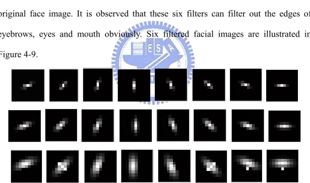
Figure 4-5 Image interpolation……….34 Figure 4-6 (a) the diagram of locating three reference points and (b) is the result…..36 Figure 4-7 Different frequencies and orientations of Gabor wavelet filters…………38 Figure 4-8 original face image ………38 Figure 4-9 Six selected filtered facial images ………...…….………….39 Figure4-10 (a) is the image by summing 6 Gabor jets. (b) is binary image of facial

edges.(c) is the intersection of 14 ROIs and the binary image of edge regions.………..….40 Figure 4-11 14 facial points………..40 Figure 4-12 The overall procedure of feature point extraction in the training phase and testing phase…………....………42 Figure 4-13 The list of AUS related to five expressions [4]…...……….44 Figure 4-14 Examples of the AR Face Database (a)neutral expression (b) smile

(c)scream (d)left light on (e)right light on (f)all lights on………47 Figure 4-15 Accurate extraction of all facial points……….48 Figure 4-16 Five categories of facial expressions under four lighting conditions…..49 Figure 5-1 Five categories of facial expressions……….55 Figure 5-2 Sample images of a new person in the experiment………56 Figure 5-3 Sample images of other five new persons in the experiment……….58 Figure 5-4 Comparison of recognition rate of proposed critical sets training algorithm

and the conventional method using all SVs in training……….…….58 Figure 5-5 The real-time vision system………60 Figure 5-6 Hardware architecture of the imaging system on Momobear……….60 Figure 5-7 HRI procedure of the proposed emotion recognition system……….……62 Figure 5-8 The designed actions of Momobear……….………...62

viii

Figure 5-9 The interaction scenario………63 Figure 5-10 An example of interaction with Momobear……….67

ix

List of Tables

Table 3-1 The relationship of decision value and Lagrangian multiplier……….23

Table 3-2 The overall procedure of proposed learning algorithm………...28

Table 4-1 The detailed descriptions of 14 ROIs………..36

Table 4-2 The definitions of 14 facial points………41

Table 4-3 The association of 5 facial expressions to AU combination………43

Table 4-4 Feature points based descriptions for AUS………..44

Table 4-5 The detailed descriptions of these 16 feature values………46

Table 4-6 The results of facial point extraction………47

Table 4-7 The results of facial point extraction in neural expression………..49

Table 4-8 The results of facial point extraction in happiness expression……….50

Table 4-9 The results of facial point extraction in anger expression………50

Table 4-10 The results of facial point extraction in surprise expression………..51

Table 4-11 The results of facial point extraction in sadness expression………..51

Table 5-1 Average recognition results of training subjects……….53

Table 5-2 Average recognition results of testing subjects………...53

Table 5-3 Average recognition results of normal light………54

Table 5-4 Average recognition results of left light on………..54

Table 5-5 Average recognition results of all light on………...…54

Table 5-6 Average recognition results of right light on………54

Table 5-7 The recognition result of the original four trained person…………..…….56

Table 5-8 The recognition rate of the 1st new facial data………..…...56

Table 5-9 The recognition rate of the 1st new facial data after learning………...57

Table 5-10 The recognition rate of all new face learning……….58

x

Table 5-12 Recognition rate of the first new person before online learning………...63 Table 5-13 Recognition rate of the first new person after online learning…………..64 Table 5-14 Recognition rate of the second new person before online learning……...64 Table 5-15 Recognition rate of the second new person after online learning………..64 Table 5-16 Recognition rate of the third new person before online learning………..65 Table 5-17 Recognition rate of the third new person after online learning………….65 Table 5-18 Recognition rate of the fourth new person before online learning……....65 Table 5-19 Recognition rate of the fourth new person after online learning………...65 Table 5-20 Average recognition results of four new persons before online learning...65 Table 5-21 Average recognition results of four new persons after online learning…..66 Table 5-22 The recognition results of five trained person after online learning……..67 Table 5-23 Recognition results of the method proposed in [41]………..67

1

Chapter 1

Introduction

1.1 Preface

In recent years, many service robots, household robots and entertainment robots have been developed for various applications [1]. One of the most important features of these robots is their human-centered functions. In the near future, intelligent service robots will have human-like interactions and work with us in our daily life. Therefore, the research of human-robot interaction (HRI) has become increasingly popular in robotics area.

In current HRI design, a variety of interaction modes including gesture, facial expression and audio have been adopted in a more natural manner. For human beings, facial expressions reveal a person’s emotion and provide important communicative cues during social interaction. This implies that facial expressions form a major modality in human robot communication.

Several research efforts on facial expression recognition (FER) have been reported recently. A set of six basic facial expressions (anger, disgust, fear, happiness, sadness and surprise) were defined by psychologists [2]. In order to make the analysis of FER more standard, facial action coding system (FACS) was created to describe the sets of facial muscle movements[3][4]. In a form of rules, FACS provides a linguistic description of all possible facial changes in terms of 44 Action Units (AUs), which can be combined to form all kinds of facial expressions.

2

expression is an essential step to make the interaction more natural and efficient. In an automatic FER system, there are three major components to achieve this goal (See Figure 1-1). First, a face is detected and localized in a camera scene. Next, relevant facial feature information from the detected face region is extracted. Finally, the facial expression category is classified based on the extracted features.

In general, most image-based recognition systems need to collect certain number of facial dataset to train the emotion classifiers. However, appearance variations of human facial expression would be too great to be represented by fixed number of samples. Thus, high recognition rate in practical robotic applications can hardly be expected with only limited datasets. Accordingly, we propose a novel solution to this problem (termed subject-dependent) by making an entertainment robot to learn incrementally through HRI and to adapt to incoming samples from a new face, which are wrongly recognized by using previous emotion classifier.

Furthermore, inaccurate feature extraction very often results in erroneous recognition of facial expression. Environmental factors such as illumination variation may cause FER system to extract feature inaccurately. In this thesis, Gabor wavelet based feature extraction is also employed to detect facial features robustly under uncertain environments.

1.2 Related Works

In past decades, many techniques have been presented in the literature related to facial expression recognition. A survey of this area can be found in [5]. The report

3

approaches can be categorized into two main directions, the feature-based methods and the template-based methods, according to the way that the facial information is extracted. Feature-based methods mainly use local spatial analysis or geometrical information as facial features. Template-based methods use holistic spatial analysis, 2D or 3D face models as templates to represent facial expression information.

1.2.1 Feature-Based Approach

A method of facial expression recognition based on selective feature extraction was proposed in [6]. Active appearance model (AAM) was applied to extract the contour of eyes, eyebrows and mouth. The displacement information of these features was classified based on selective feature rule. Another method proposed in [7] overcame some limitations of current HRI techniques, such as their sensitivity to partial occlusion and noisy data. This method features a representation of facial expressions which combines spatially-localized geometric facial model with state-based model of facial motion. Through the transition of feature states, this method reduces influences of noise and occlusion.

Gabor filters are popular in representing facial features. The results in [8] revealed that Gabor features from different Gabor channels have different contributions to the facial expression recognition. Therefore, [8] proposed a method to improve the performance of recognizing facial expressions by combining features belonging to different channels.

A fast and robust facial expression recognition design using video stream was proposed in [9]. In the first frame of the face video, 20 facial points were extracted from each region of interest in face region by using GentleBoost templates built from Gabor wavelet features. Then, a particle filter was exploited to track points in the subsequent image frames. AdaBoost selected the most informative spatio-temporal

4

features to train a support vector machine (SVM) classifier.

Facial expression recognition using small number of training samples was reported in [10]. An algorithm called feature selection via linear programming (FSLP) was proposed to select features efficiently. In [10], probability distribution based learning methods were compared with margin based methods for the case of small number of training examples. It was reported that the margin methods such as FSLP and SVM [11-12] have more accurate facial classifying results than those based on probability distribution, such as Bayes classifier and AdaBoost in the small sample cases.

Another spatio-temporal approach to recognize six facial expressions from visual data attempted to measure levels of interest from video [13]. It used projected optical flow vectors as facial features and applied principal component analysis (PCA) to reduce the dimension of optical flow. Discrete hidden Markov Models were used to learn the classifying model for each facial expression. Finally, the third dimensional affect space was also adopted to combine facial motion information around apex frame in order to guarantee the performance of facial expression recognition. In [14], a set of muti-scale and muti-orientation Gabor wavelet coefficient extracted from face images at fiducial points were adopted to represent the facial features. These features were fed to the input units of the two layer classifier.

1.2.2 Template-Based Approach

In [15], facial expression recognition system was reported to be subject-independent and robust against illumination variation and image deformation. In their method, Gabor features at each lattice of expression image constructed an elastic graph. The amplitudes of those feature vectors tended to be larger at some key lattices. Expression recognition was performed by template matching of features and

5 position of key-points.

An approach to recognizing gender and facial expression was proposed in [16]. AAM was used to extracted facial features [17]. Features extracted by a trained AAM were classified by a SVM. Gender-specific classification cascading facial expression classification were considered to yield better performance of classification.

Two real-time methods for facial expression recognition in image sequences were proposed in [18]. Some of Candide grid’s points in face region were depicted manually at the first image sequences. The grid tracking system based on deformable models tracks all grids of expressional face in the remainder image sequences until the image frame reached the greatest facial expression intensity. The geometrical displacement of those Candide nodes were used as input to a muticlass SVM classifiers, which recognize the six basic facial expressions and a set of Facial Action Units.

The related works mentioned above mainly focus on algorithms or methods to improve the recognition performance. Few papers involve in the research of learning new facial data in online robotic applications. Recently, a method of expression learning was proposed by imitating the process of a baby’s learning process [19]. A penguin robot started learning three facial expressions by recognizing human actions through CdS light sensors equipped on the robot’s head. After learning new facial expressions, the penguin robot could identify the emotions without using the CdS light sensor.

Although few papers concern about expression learning, incremental learning for online face recognition, a similar procedure to facial expression recognition, has drawn much attention in recent years. In [20], a new approach to face recognition in which not only a face classifier but also a feature space was learned incrementally to adapt to new incoming samples. To learn a feature space and an optimal decision

6

boundary in online, an extended version of incremental principal component analysis (IPCA) and resource allocating network with long-tern memory (RAN-LTN) were combined to achieve this goal. For using IPCA, a feature space was updated to a new training number by rotating its eigen-axes and increasing its dimensions. In RAN-LTM, a small number of training samples called memory items were selected for retraining a new classifier. The face recognition system was adapted to a new face incrementally by learning a new feature space and a face classifier online.

The architecture suitable for real time robotic learning of face recognition was proposed in [21]. A face tracking coupled to a clustering technique was utilized to learn a person’s face appearance when the system interacted with a user. The learning approach is similar to the partial memory incremental learning method, where the representative samples of similarity measurement can be updated for new incoming faces.

According to the survey of facial expression and learning, we hope a robot to learn facial expressions incrementally. Further, a good and adaptive classifier is essential for online learning. Support vector machine (SVM) has been an effective method for designing facial expression recognition systems, especially when the training samples are small [10]. Therefore, online robotic learning of new facial data has become the problem of SVM-based incremental learning in this study.

A popular method to expedite SVM learning is to reduce the number of training data. Vanik [11][12] showed that the training result of SVM depends only on a small set of samples, termed support vector (SV) sets. Chunking algorithm [12] solved the SVM containing all SV sets plus some new samples which violate the Karush-Kuhn-Tucker (KKT) condition. Decomposition method [12] is similar to the Chunking algorithm. The main difference is that the size of retraining samples in decomposition method is fixed. In addition to these conventional methods, α-ISVM

7

[22] provides an efficient incremental algorithm based on the discard factor α. Through the adjustable parameter, it is possible to discard samples optimally. Thus retraining time of SVM can be saved greatly. Another incremental learning algorithm I-SVM [23] also discarded part of history samples, both the pre-extracting SVs algorithm and the iteration algorithm have been used in the retraining of the SVM. SeqSVM [24] trained a SVM classifier on a small part of training samples and selected the so-called convex hull samples, which were wrongly classifier by the current SVM, to retrain a new SVM.

1.3 Problem Statement

Note that the incremental learning methods described above need old training data of the SV sets. In order to make an original SVM emotional classifier to adapt to new subjects’ facial expressions, one intuitive incremental learning approach is to store old SV samples in memory and retrain all of them, including the new samples. However, this approach will lead to a problem that if the number of retraining data is large, it will require much time to solve quadratic optimization (QP) to obtain a SVM classifier[11][12]. The training time will increase dramatically with the number of training dataset, resulting in inefficiencies in practice from both memory requirement and real time criteria. To assure that the robot can accommodate its emotion recognition system to a new human face effectively, a fast incremental learning algorithm for emotion recognition is desired.

Inaccurate feature extraction will result in erroneous recognition of facial expressions. In practical applications, feature extraction may fail due to lighting conditions of the environment because gray values suffer from huge ambiguities as well as slight changes in illumination. Therefore, how to extract facial features robustly under illumination variation conditions is still a problem in facial expression

8 recognition.

1.4 System Overview and Organization of the Thesis

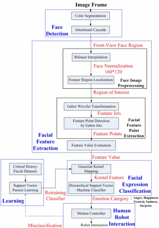
The architecture of the proposed system is shown in Figure 1-2. The system consists of five units, namely face detection, facial feature extraction, facial expression classification, human-robot interaction and facial classifier learning.

First, a face region is detected under illumination variation conditions. Next, in order to improve the efficiency of feature extraction, the front-view face region is preprocessed by normalizing the face and localizing the feature region before feature extraction. Gabor wavelet based features regardless of illumination variation are used to detect the facial fiducial points in the relevant region of interest. After extracting those feature points, the feature values are evaluated from the geometric displacement of facial points according to FACS. Third, five categories of facial expression, neutral, anger, happiness, sadness and surprise are classified by hierarchical SVM classifiers. An entertainment robot can response to the estimated emotions. If an entertainment robot recognizes the user’s facial erroneously, a fast SVM-based learning algorithm is employed to adjust the SVM classifier. The incremental procedure is executed to learn facial expressions of new individuals. A novel algorithm using support vector pursuit learning (SVPL) coupled to critical historical sets to restrain a new SVM classifier in Gaussian feature space is designed to make the robot achieve this goal.

The rest of this thesis is organized as follows. In chapter 2, SVM-based classifier is introduced. Chapter 3 describes the classification of facial expressions and the proposed learning algorithm of SVM classifier. In chapter 4, a robust facial feature extraction insensitive to illumination is introduced. In chapter 5, the experimental results of the proposed algorithm are presented and discussed. Chapter 6 summarizes the contribution of this thesis and gives directions of further research.

9

10

Chapter 2

SVM-Based Classifiers

The emotional classification and the learning algorithm of an entertainment robot have been developed based on SVM, a statistical learning theory. We will introduce the basic principle of SVM in this chapter.

2.1 Support Vector Classification

Support Vector Machine [11][12] is a popular machine learning technique based on statistical learning theory and structural risk minimization principle. SVM has become increasingly popular in many fields. SVM has been successfully applied in many applications such as pattern recognition, multi-sensor information fusion and bio-sequence analysis.

2.1.1 Linear SVM

The simplest model of Support Vector Machine is the maximal margin classifier. It works only for data which is linearly separable in the feature space.

Given a set of training samples belonging to two classes, } , {xi yi , =1,..., , ∈ , i ∈{±1} n i R y x l

i , the goal of SVM is to find a hyperplane

0 = + •x b

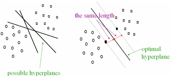
w to separate the data successfully. In general, SVM classifiers separate the data with the maximal margin hyperplane. Figure 2-1 shows that there are many possible hyperplanes to separate the data, but only one can maximize the margin between two classes.

11

Figure 2-1 The optimal hyperplane of SVM

For the linearly separable case, all the training data satisfy the following constraints [12]： 1 ≥ + • + b x w for yi =+1 (2-1) 1 − ≤ + • − b x w for yi =−1 (2-2)

The geometric margin γ can be maximized by computing the following function： 2 2 2 2 _{|| ||} 1 ) ( || || 1 ) || || || || ( w x w x w w x w w x w w _{• >−< • > = < • >−< • > ∝} < = + − + − γ (2-3)

Hence, an optimal hyperplane which gives the maximum margin by minimizing

2

||

|| w can be found. Similarly, the hyperplane (w,b) can be solved by the following optimization problem： Minimize w,b <w•w>, (2-4) Subject to ( • + + )≥1 b x w yi i , i=1,...,l, (2-5)

This optimization problem can be solved by finding the saddle point of the Lagrangian. The primal Lagrangian is

max

_∑

= − + • − = l i i i i y w x b w b w L 1 2 _{{ ( ) 1}} || || ) , , ( α α (2-6) where α_i ≥0 are the Lagrange multipliers. The corresponding dual is found by differentiating w and b, and the solution can be written as follows：

12

∑

= = ⇒ = ∂ ∂ l i i i i y x w w b w L 1 0 ) , , ( α _{α (2-7)}

∑

= = ⇒ = ∂ ∂ l i i i y b b w L 1 0 0 ) , , ( α _{α (2-8)}

Substituting the relations into (2-6) to obtain the following dual objective function:

max

∑

= − + > • < − > • < = l i i i i y w x b w w b w L 1 ] 1 ) ( [ 2 1 ) , , ( α α (2-9)

∑

∑

∑

= = = + > • < − > • < = l j i l i i j i j i j i l j i j i j i j iy x x y y x x y 1 , 1 1 , 2 1 _{αα αα α (2-10)} α α α α α α y y x x T TD l j i j i j i j i l i i 2 1 2 1 1 , 1 − = > • < − =

∑

∑

= = (2-11) To maximize the equation, the Lagrange multipliers α_i can be obtained by differentiating (2-11). After substituting ₌ −1_•1

D

i

α into (2-7), the parameter of SVM hyperplane w can be solved. Although the value of b does not appear in the dual problem, b can be solved by using the constraints：

2 ) ( min ) ( max ₁ < • > + ₁ < • > − = yi=− w xi yi= w xi b (2-12) 2.1.1.1 Support Vectors

In addition, the Karush-Kuhn-Tucker (KKT) conditions play an important role in the structure of the solution [12]. The KKT conditions state that the optimal solutions α ,(w, b) must satisfy： 0 ] 1 ) ( [y_i <w•x_i >+b − = i α , i=1,...,l. (2-13) This equation implies that x , which decision value is one, has corresponding i

non-zero αi . According to (2-7), the parameter w is involved mostly with these

13

Figure 2-2 A maximal margin hyperplen with its support vectors

shows that there are many vectors in the plane, but only few lie on the dotted line and form the SVM hyperplane.

2.1.2 The Non-Separable SVM

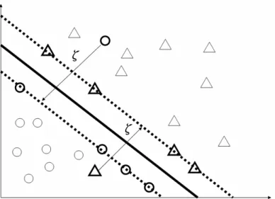
The above algorithm is for separable data, but it will find no feasible solution when the data in the feature space are non-separable [12]. 2-Norm Soft Margin SVM

is introduced to separate the data that are not linearly separable in the feature space. In

order to solve this non-separable case, positive slack variables ξ_i,i=1,...,l. are used to make the constraints to be violated (See Figure 2-3)：

Minimize w,b

∑

= + > • < l i i C w w 1 2 ξ , (2-14) Subject to y_i(w •x_i+ +b )≥1−ξ_i, i=1,...,l, ξ_i >0 (2-15)

whereξ is slack variables and C is a constant which determines the trade-off _i between training error and VC-dimension. Then, this optimization problem can be solved by finding the saddle point of the Lagrangian：

max

_∑

_∑

= = + − + • − + = l i i k i k k i k i l i i y w x b C w L 1 1 2 2 _{{ ( ) 1 }} 2 1 || || 2 1 _{ξ α ξ (2-16)}

14

Figure 2-3 Linear separating hyperplane for the non-separable case.

where α_i ≥0 are the Lagrange multipliers. The solution can be written as follows：

∑

= = ⇒ = ∂ ∂ l i i i i y x w w L 1 0 α (2-17)

_∑

= = ⇒ = ∂ ∂ l i i i y b L 1 0 0 α (2-18) =0⇒ − =0 ∂ ∂ _{ξ α} ξ c L _(2-19)

Substituting the relations into (2-16) to obtain the following dual objective function

∑∑

∑

= = = • − • + + • − = l i l j l i i j i j i j i k C C x x y y D 1 1 1 ) ( 1 ) ( 2 1 ) ( 2 1 ) ( max α α α α α α α α

∑∑

∑

= = = • − + • − = l i l j l i i j i j i j i C x x y y 1 1 1 ) ( 2 1 ) ( 2 1 _{α α α α α (2-20)}

Hence, maximizing the above objective function over α is equivalent to maximize

) 1 ( 2 1 ) , , , ( 1 , 1 ij l j i j i j i j i l i i C x x y y b w L ξ α =

∑

α −

∑

αα ⋅ + δ = = (2-21) where ⎩ ⎨ ⎧ = = others j i if ij 0 1 δ (2-22) After substituting k i

α in (2-17), the parameter of the hyperplane w is solved. The value of b is chosen using the relation αi = Cξi and referred by

15

Karush-Kuhn-Tucker complementarily condition. The condition is as below

(

)

(

_i ⋅ _i + −1+ _i

)

=0

i y w x b ξ

α ∀i (2-23)

2.1.3 Non-linear SVM

SVM also can generalize to the case where the decision function is not a linear function. This problem can be solved by mapping the data from the feature space to some other higher dimension space (possibly infinite dimension). In most cases of SVM, several kernel functions have been used for nonlinear mapping. Three kernel functions are the most commonly used, and those are

Polynomial： T d r x x x x K( ₁, ₂)=(γ _{1 2} + ) , r>0 (2-24) Sigmoid：K(x1,x2) tanh( x1 x2 r) T ₊ = γ (2-25)

Gaussian radial basis function： ( , ) exp( || || )

2 2 1 2 1 c x x x x K = − − (2-26) where γ , d, c are kernel parameters. In these kernel functions, kernel space is infinitely dimensional, so we do not need to know the mapping space of a kernel function explicitly. In conclusion, for a given kernel function, the non-linear decision function of SVM classifier can be now written as

) ) ( ( ) ( 1 b x x K y sign x f _i l i i i • + =

∑

= α (2-27) where x_i are the support vectors.

2.2 Incremental SVM

16

classifier. The key point is that obtaining αi of the dual objective function is time

consuming because it involves in the computation of matrix inverse in the programming procedure. So the training time will increase dramatically with the number of training dataset. On the other hand, SVM also suffers from the problem of large memory requirement when training on a large data set. Therefore, incremental learning techniques are developed to make the SVM training faster and to reduce the storage cost over very large data sets.

According to (2-13), the training result of SVM only depends on a small set of samples, termed support vector (SV) sets [11-12]. Therefore, Chunking algorithm [12] solves the SVM incrementally containing all SV sets plus some of new samples which violate the Karush-Kuhn-Tucker (KKT) condition. But the shortcoming is that the algorithm is limited by the maximal number of support vectors and still requires the procedure of the quadratic optimization. Decomposition method [12] is similar to the Chunking algorithm. The main difference is that the size of retraining samples in decomposition method is fixed.

Except for these conventional methods, α-ISVM [22] provides an efficient incremental algorithm based on the discard factor α. Through the adjustable parameter, it is possible to discard samples optimally. Thus retraining time of SVM can be saved greatly. Another incremental learning algorithm I-SVM [23] also discards part of history samples, both the pre-extracting SVs algorithm and the iteration algorithm have been used in the retraining of the SVM.

SeqSVM[24] trains a SVM classifier on a small part of training samples and selects the so-called convex hull samples to retrain a new SVM. Convex hull samples are wrongly classified by the current SVM and furthest from the current SVM solution. It implies that these samples are the most possible to be the support vectors in the future

17 SVM.

Some other traditional methods of SVM-based incremental learning [25-26] also expedite the retraining by reducing the number of the training data. Besides reducing the number of retraining samples for the purpose of speeding up the retraining procedure, Sequential Minimal Optimization (SMO) [12] provides an alternative approach to avoid the overall procedure of QP. SMO is derived by taking the idea of decomposition method to its extreme and just optimizes two multipliers α₁ and α₂

in each QP sub-problem. We can compute new values of the two multipliers by keeping the linear constrain

∑

= = l i i iy 1 0

α and the new multipliers have the following relationship： 2 2 1 1 2 2 1 1y y constant y y old old _α α α α + = = + (2-29) The choice of updating the two multipliers is determined by a heuristic. The procedure of SMO is closed while all Lagrange multipliers satisfy the KKT conditions.

Note that the incremental learning methods described above mostly need old training SV sets. Therefore, if we want to train a SVM which can classify new learning datasets and keep the performance of recognizing old ones, retraining new data together with SV set of the original samples or many historical sets would be necessary. This would be insufficient for real-time criteria and memory requirement in robotic applications. To this end, we will propose a fast SVM-based learning algorithm to expedite the training of SVM.

18

Chapter 3

Facial Expression Classification and

Learning

This chapter describes the developed classifier and learning algorithms of a robotic facial expression recognition system. SVM is applied to the proposed system for recognizing five facial expressions. Generally, an image-based facial expression recognition system needs to collect certain number of facial datasets to train the emotion classifiers. This will lead to a problem that appearance variations of human faces would be too great to be represented by limited number of samples in practical applications. This means that high recognition rate in practical robotic applications can hardly be expected with only few dataset. Therefore, we propose a novel incremental learning algorithm based on SVM to overcome the problem (termed

subject-dependent) of facial expression recognition.

The basic idea of the proposed learning algorithm is to adjust parameters of the SVM hyperplane for learning facial expressions of a new face, which is defined as the data recognized incorrectly through previous trained SVM classifiers. Support vector pursuit learning (SVPL, see 3.2.1) [27-28] is applied to retrain the hyperplane iteratively in the Gaussian-kernel space. To expedite the retraining procedure, only erroneous samples are combined with critical historical sets (see 3.2.2) to restrain a new SVM classifier. After the fast retraining using the proposed method, the new classifier will learn to recognize new facial data with improved correct rate.

19

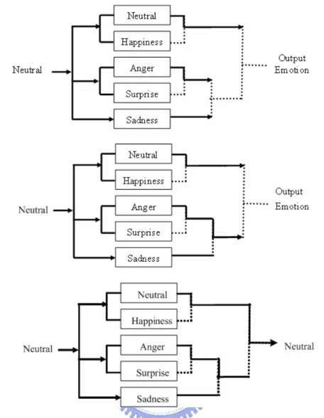
3.1 The Hierarchical SVM Classifier

It is well known that SVM has been an effective method for designing facial expression recognition system [10], especially when a small number of training data are considered. For using SVM classifiers, the categories of two-class data can be decided by computing the sign of the decision function. The facial expression classifier needs to recognize five categories of emotional expressions consisting of anger, happiness, neural, sadness and surprise. Consequently, a hierarchical SVM classifier is designed to categorize five emotional expressions. The structure of hierarchical SVM classifier is as shown in Figure 3-1. An example of classifying a neutral expression is also illustrated in Figure 3-2. First, neutral, anger and sadness are performed through the first layer classification. Next, anger expression assumes sadness expression in the second one. Finally, neutral expression can assume sadness and be outputted through three layer classifications.

3.2 Fast Learning for Robotic Applications

A facial expression recognition system needs to collect some representative

Figure 3-1 The structure of hierarchical SVM classifier. Neutral Happiness Anger Surprise Sadness Output Emotion Input Unknown Emotion

20

Figure 3-2 An example of classifying neutral expression

samples to train SVM classifier beforehand. The subject-dependent problem in facial expression recognition can hardly be avoided because different people may show a categorized expression in different ways. If the facial expressions of a test person are not collected previously in the database, high recognition rates are difficult to obtain. Therefore, a solution to this problem is investigated to accommodate the robot to various persons’ facial expressions.

The objective of this study is to design a system for emotional interaction of entertainment robots. An entertainment robot equipped with a facial expression recognition system and learning algorithm can recognize the facial expression of its

21

host. For a newly purchased robot, if the robot recognizes new faces correctly, then the current parameters of the recognition system will be good enough. On the contrary, if the owner perceived that the robot recognizes new facial expressions erroneously by observing the emotional responses of the robot, the owner would inform the robot about the wrong recognition results through a simple input device. Consequently, the entertainment robot can start to retrain a new SVM hyperplane immediately.

As mentioned in Chapter 2, large sizes of retraining samples will require much time to solve quadratic optimization (QP) of a SVM classifier. This would not be efficient in practice from both memory requirement and real time criteria. So a fast SVM-based incremental learning algorithm will be required for practical applications.

3.2.1 Support Vector Pursuit Learning

We adopt the concept of support vector pursuit learning (SVPL) [27-28] to develop the emotion learning system. Previous parameters of the hyperplane together with the new data are employed to restrain a new SVM classifier. The main idea of SVPL is that the old hyperplane k−1

w shifts a minimal distance to a new

hyperplane k

w in order that the new one can separate new data correctly (See Figure

3-3). The data in Figure 3-3 are all new training samples. Because the distance between the new and previous hyerplane is minimal, the new hyperplane is also expected to separate the old data. When the new classifier is obtained, the new training data of the current step can be discarded after completing the training procedure. Hence SVPL effectively reduces the competition and the memory requirement in learning new data.

In practical applications, facial expressions of new faces, which will be learned incrementally, are usually far different from the original ones. It will result in that the

22

Figure 3-3 The diagram of SVPL retraining strategy

new SVM will not maintain a satisfactory performance of recognizing the old data. So we propose to use a new concept of critical sets to couple with SVPL to design a learning algorithm to achieve this goal.

3.2.2 Critical Sets

Gaussian-kernel mapping method is added in the first stage in the developed algorithm to map the feature space to kernel space where facial data can be retrained easily. Gaussian radial basis function is written as follows：

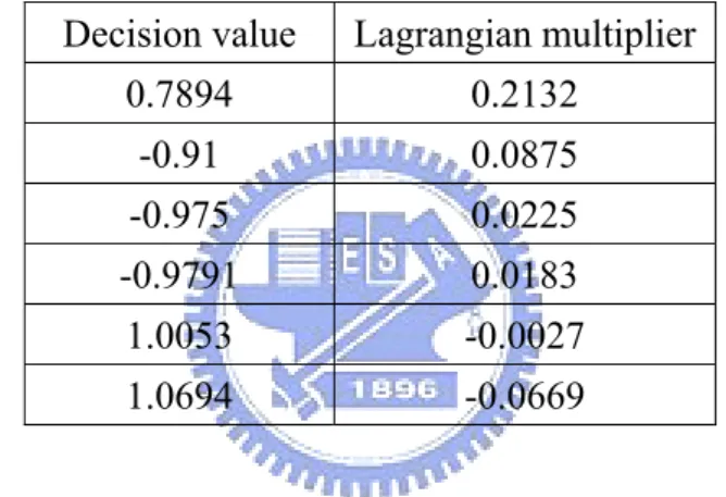
) || || exp( ) , ( 2 2 1 2 1 c x x x x K = − − (3-1) Subsequently, as described in (2-7), the hyperpleane w is constructed from the summation of feature values and the class category. Lagrange multiplierα_i determines weights of the training samples to form the hyperplane w. In general, the samples which are nearest to the SVM hyperplane have greatest values of Lagrange multipliers. Namely, these samples play critical roles in forming the SVM hyperplane. This concept can be explained using Figure 3-4. Figure 3-4 (a) shows that a SVM is

23

(a) (b)

Figure 3-4 (a) a SVM trained with all samples (b) a similar SVM trained with critical sets

Table 3-1 The relationship of decision value and Lagrangian multiplier Decision value Lagrangian multiplier

0.7894 0.2132 -0.91 0.0875 -0.975 0.0225 -0.9791 0.0183 1.0053 -0.0027 1.0694 -0.0669

trained with all samples existing in the feature space, but one can also train an almost the same SVM with few sets that are as shown in Figure 3-4 (b). On the other hand, Table 3-1 shows an example that the sets whose absolute decision values are smaller have bigger Lagrangian multipliers.

As a result, a few historical and important samples, which are nearest to the SVM hyperplane, are reserved to restrain a new SVM classifier for keeping the recognition of old data. We define these samples as critical sets (CSs).

CSs： Xi =argmin|w•Xi+b| (3-2)

The size of critical sets is determined empirically. There is a trade-off between training time and the size of critical sets. Thus, we can adjust the size of critical sets to

24

meet the seesaw between learning time and non-forgetting learning.

The effectiveness of critical sets to maintain the performance of recognizing old data is shown in Figure 3-5. Assume that the hyperplane trained with the white circles and the white triangle, as shown in Figure 3-5 (a) and the black samples are new samples. It can be seen that there are two new black circles classified erroneously by the original hyperplane. Figure 3-5 (b) shows one possible retraining error risk with traditional SVPL, where the new hyperplane can classify the new samples correctly, but still one old sampe(white triangle) is misclassified. Next is a new strategy to retrain SVM, only the two erroneous black points combined with critical sets are used to retrain a new hyperplane with SVPL. One black triangle becomes the new critical set after online updating the CSs. The result of the new hyperplane is shown in Figure 3-5 (c). It can separate both the new and old samples correctly.

3.2.3 The Proposed Learning Algorithm

This section introduces the proposed learning algorithm that utilizes CSs and SVPL to retrain a SVM. We denote critical sets as L

i i i y x TS 1 0 0

0 ={ , }= which are nearest to the

initial hyperplane. At t-th incremental learning step, some new samples m i t i t i k x y TS ={ , }=1

come in, and we assume that the initial SVM cannot classify these new samples correctly. The parameters of the new hyperplane that can separate new sample successfully can be changed to( t, t)

b

w by proposed algorithm. The following steps are similar to the conventional SVM procedure, the quadratic programming problem of the incremental updating can be expressed as follows：

Objective function：

∑

+ = − ₊ − ( ) 1 2 1_|| || 2 1 min m L i i t t C w w ξ (3-3) s.t. t t _i i t i w x b y ( • + )≤1−ξ for y_i =−1 (3-4) i t t i t i w x b y ( • + )≥1+ξ for y_i =+1 (3-5)

25 (a)

(b)

(c)

Figure 3-5 An example of the retraining with critical sets by SVPL. (a) is the original SVM hyperplane, (b) one possible error of retraining all new samples by SVPL, (c) retraining only the two erroneous black points combined with critical sets by SVPL

26

whereξ is slack variables in the sets of _i TS₀ and TSk. C is a trade-off between

training error and VC-dimension. Let t−1

W denotes the previous trained parameter and a fixed constant. This optimization problem can be solved as follows：

∑

+ = − ₊ = ⇒ = ∂ ∂ ( ) 1 1 0 L m i t i t i t i t t t w w y x w L α (3-6)

∑

+ = = ⇒ = ∂ ∂ ( ) 1 0 0 m L i t i t i t y b L α (3-7) L t C i m i i ..., 1 , 0 0⇒ ≤ ≤ = = ∂ ∂ _α ξ (3-8) The procedure to solve αt is similar to 2-Norm Soft Margin SVM [12]. After

substituting α in (3-6), the parameter of the new hyperplane t k

w is solved. (3-6)

indicates that the new parameter of SVM can be derived iteratively through the parameter of previous SVM and the retraining sets comprising TS₀ and TSk .

Consequently, a new SVM, which not only recognizes new facial data but also keeps an acceptable recognition rate of original facial data, will be achieved by the proposed learning algorithm. Further, the proposed algorithm speeds up the QP procedure of SVM dramatically by reducing the retraining datasets. This is beneficial to the real-time requirement in practically robotic applications.

Finally, the decision function can be written as below： ( ) ( ( ) ) 1 b x x K y sign x f _i l i i i • + =

∑

= α (3-9)

where K(,) is a Gaussian kernel function which can be used to map the input space to some higher dimensional kernel space. Suppose that φ:X−>F is a non-linear

mapping from the input space to some higher kernel space, the decision function can be rewritten as ： ) ) ( ) ( ( ) ( 1 b x x y sign x f _i l i i i < • >+ =

∑

= ϕ ϕ α (3-10) where

_∑

= = l i i i iy x W 1 ) ( φ

27

3.2.4 Decomposing Kernel Function

Kernel function is an implicit mapping from feature space to kernel space, the underlying feature mapping is not known explicitly. Hence, w can not be derived directly for the purpose of retraining SVM hyperplane incrementally.

We can take the feature mapping to be any linear transformationx→AX, for some

matrix A. In this case the kernel mapping is given by

K

Az

A

x

Az

Ax

z

x

K

(

,

)

=<

,

>=

'

'

=

(3-11) where K is a square symmetric matrix, K can be diagonalized into the following expressions：

'

)'

(

)

'

(

'

2 1 2 1 2 1 2 1

X

X

V

V

V

V

V

V

K

=

Λ

=

Λ

Λ

=

Λ

Λ

=

•

(3-12) where 2 1 Λ = V

X . We assume that X is one possible result of kernel mapping, thus the

parameter of w can be derived explicitly. The final decision function in kernel space is given below： b X w b X X y sign b X X y sign b x x K y sign x f _i l i i i i l i i i i l i i i • + = • + = • + = • + =

∑

∑

∑

= = = ) ( ) ( ) ) ( ( ) ( 1 1 1 α α α (3-13) where i l i i iy X w

∑

= = 1

α . Diagonalizing kernel matrix to know the kernel space, the proposed learning algorithm can be accomplished even though the kernel function is an implicit mapping function. The architecture of the proposed learning algorithm is illustrated in Figure 3-6. Table 3-2 summarizes proposed learning algorithm. First, features of facial expression sample are collected. They are mapped to Gaussian kernel space. Next, a hierarchical SVM classification is used to categorize five emotion expressions. In the meanwhile, the parameter of SVM and critical sets are reserved for future learning. If new data are supplied, a new SVM classifier will be learned by the proposed algorithm, which uses only erroneous data and critical sets to

28

update the SVM. As soon as the new SVM is adjusted, critical sets are updated accordingly. The learning procedure is continued until no new data exists.

Table 3-2 The overall procedure of proposed learning algorithm

Figure 3-6 The flowchart of proposed learning algorithm

Initial ：Train the SVM classifier S1 with training facial datasets IS (initial sets) and save CS (critical sets);

Step1：Test the new facial data NS with classifier S1,

if erroneous data=Nil

then：

do nothing and exit;

else erroneous data=ES(erroneous sets)

then：

retrain new SVM classifier S with proposed learning algorithm using ES and CS ;Update CS;

Step2 ：New SVM classifier S1=S;IS=NS+IS; Step3 ：Test IS with S1;

29

Chapter 4

Feature Extraction Under Illumination

Variation

To assure that feature values are extracted accurately for classification and learning, we adopt Gabor wavelet to develop a robust feature extraction method. Facial points can be detected under various lighting conditions. Before extracting facial features, a face should be localized and segmented from digitized images sequences. Face preprocessing stage consists of face normalization andfeature region localization steps to extract facial features efficiently. While regions of interest corresponding to relevant features are determined, we apply Gabor jets based on Gabor wavelets transformation to extract the facial points. Gabor jets are more invariable and reliable than the gray values which suffer from huge ambiguities as well as slight changes in illumination while representing local features. Each feature point can be matched by a phase-sensitivity similarity function in the relevant regions of interest. As long as the feature points are extracted under illumination variety, we can evaluate the geometric displacements of these points as emotional feature values.

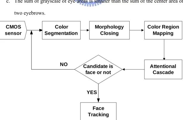
4.1 Face Detection

Color is a direct cue for face localization, but skin color is easily suffered from illumination uncertainty. In this design, a YCrCb 3D color distribution model is applied to segment skin color under illumination variation [29]. The method of face localization consists of face detection and face tracking. Face detection module is an initial state which contains the location and size of face information for latter face

30

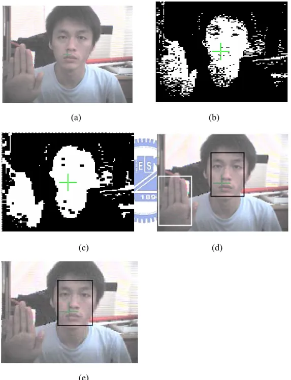
tracking. Face region is detected in the first image of image sequences by executing face color segmentation, morphology, color region mapping and attentional cascade (see Figure 4-1).

As shown in Figure 4-2 (b), the binary image is obtained by using skin color segmentation in YCrCb color space. Then, closing operation of morphology [30] is used to eliminate the discontinuous interference in the skin color region(see Figure 4-2 (c)). After obtaining the binary image of color segmentation, the 2-D histogram mapping is utilized to find possible areas of faces and Figure 4-2 (d) illustrates the result. Finally, attentional cascade assigns several rules to confirm if the candidate region is a real human face. If the following conditions are satisfied, the face detection is regarded successful：

a. The ratio of mapping length to mapping width is between 1 and 2.

b. The sum of grayscale in the upper area is smaller than the sum of the lower one.

c. The sum of grayscale of eye areas is smaller than the sum of the center area of two eyebrows. CMOS sensor NO _{Candidate is} face or not YES Color Segmentation Morphology Closing Color Region Mapping Attentional Cascade Face Tracking

31

d. The sum of grayscale of the adjacent cheek areas is less than one fixed threshold.

One successful example is shown in Figure 4-2 (e).

(a) (b)

(c) (d)

(e)

Figure 4-2 The results of face detection (a) is the testing image. (b) is the result of color segmentation and (c) is the result of closing operation. (d) is the candidate of face regions. (e) is the final result via the attentional cascade.

32

4.2 Face Tracking

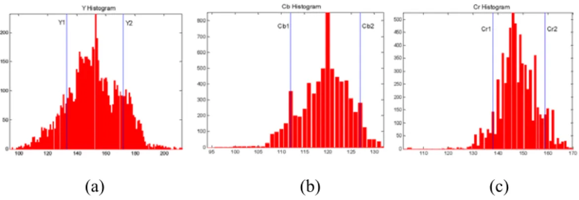
After a face is detected in the initial state, face tracking can be accomplished in the subsequent images by applying the adaptive YCrCb 3D color distribution model. This statistical model determines the proper threshold values for each color channel of the face image in the tracking mode. Let Y1(Y2) be lower(upper) threshold of skin color of Y channel, Cr1(Cr2) be lower(upper) threshold of skin color of Cr channel and Cb1(Cb2) be lower(upper) threshold of skin color of Cb channel. The threshold values used to segment the face regions are updated by the following equations[29]：

] 0 min max )) ( min[( arg 2 > = × − =

∑

C C i S total N i hist C i C (4-1) 0 ] max min )) ( min[( arg 1 > = × − =

∑

C C i S total N i hist C i C (4-2)

Where C denotes the channel of color spaces, Y, Cr or Cb and Chist is the histogram of the C channel. S is a scale factor from 0 to 1 to reject the undesired histogram such as eye or eyebrow; in this case the scale factor is set to 0.1. Ntotal is the total pixel number of previous face region. Figure 4-3 shows an example of computing the threshold values. The face tracking method utilizes the color distribution model to update the threshold values of skin color from the previous face region of sample instant t-1. The threshold values can be adjusted dynamically to accommodate the unexpected changes of lighting conditions.

4.3 Face image preprocessing

To improve the efficiency of extracting facial features, we perform face image preprocessing including face normalization and feature region localization. The segmented front-view face region is firstly normalized to 160x120 grayscale image.

33

(a) (b) (c)

Figure 4-3 The lower and upper thresholds of each color channel (a) Y1 and Y2 of Y channel (b) Cb1 and Cb2 of Cb channel (c) Cr1 and Cr2 of Cr channel

Three reference points are found on both pupils of the eyes and at the center of the mouth. As shown in Figure 4-4, the face region is divided into 14 relevant regions of interest (ROI), each containing one feature point.

4.3.1 Face normalization

Face region is normalized to a 160x120 gray-value image by using bilinear interpolation [30]. Image bilinear interpolation estimates function value f(x',y') based on the known values of nearby pixel f( yx, ). As shown in Figure 4-5, assume that the black points are unknown values and we estimate them linearly by using the

34

Figure 4-5 Image interpolation

known white points. The bilinear interpolation function can be expressed as follows：

)] 1 , ( ) , ( ) 1 )[( 1 ( ) ' , ' (x y = − −u f x y +uf x y + f

λ

)] 1 , 1 ( ) , 1 ( ) 1 [( − + + + + +

λ

u f x y uf x y _(4-3) where,

x

x

x

x

−

−

=

'

λ

,

y

y

y

y

u

−

−

=

'

4.3.2 Feature Region Localization

For feature extraction, the relevant regions of interest are determined first. Three reference points located on both pupils of the eye and at the center of the mouth are detected for this purpose by using an adaptive threshold method, integral optical density (IOD) [31]. The pupils are supposed to be the darkest in the upper face regions, so the binary image of the pupils can be segmented by selecting a proper threshold. However, the entire gray-values of the face may vary from image to image, and a fixed threshold does not acquire the binary image of pupils successfully. Consequently, to overcome this problem, IOD is employed to adaptively determine the threshold. The IOD is defined as ：

35

∫∫

∫∫

= D D k dxdy dxdy y x Y IOD ) , ( (4-4)

where

Y

_k

( y

x

,

)

is binary image with a certain threshold value k.

In this design, the binary image of the pupils is segmented with the value of IOD set to 0.05 in the rectangle area of 30x30 pixels. Namely, we choose 5% of the darkest gray-value to locate the positions of the pupils. The positions of these two rectangle regions are illustrated in Figure 4-6 (a). In this case, the coordination of the left pupil region is from pixel(15, 40) to pixel(45, 70). The coordination of the right pupil region is defined from pixel(75, 40) to pixel(105, 70). After obtaining the binary image of the pupils, we use 2D-hisgram mapping to locate the positions of the pupils accurately. On the other hand, the center of the widest peak will define the vertical position of the middle of the mouth between pix100 to pix150 in the vertical direction, and the horizontal position of the mouth is the center of two pupils. In this way, three reference points can be found. Figure 4-6 (b) shows typically detected result of these points.

Subsequently, we utilize these three reference points to further divide the face region into 14 regions where each facial point is extracted individually. The detailed descriptions of 14 ROIs are given in Table 4-1.

4.4 Gabor Wavelet Transformation

Features based on Gabor filters have been used in image processing due to their powerful properties [32-35]. In particular, the most favorite one is to remove the variability in lighting, rotation, small shift or deformation in the local feature areas. In this thesis, we will apply Gabor wavelets-based features instead of grayscale features to extract facial points.

36

(a) (b)

Figure 4-6 (a) the diagram of locating three reference points and (b) is the result

Table 4-1 The detailed descriptions of 14 ROIs ROI-1 Range from pixel(R3_x-8,R3_y-18) to pixel(R3_x+8, R3_y-3). ROI-2 Range from pixel(R3_x-8,R3_y+3) to pixel(R3_x+8, R3_y+30). ROI-3 Range from pixel(R3_x+15,R3_y-10) to pixel(R3_x+40, R3_y+10). ROI-4 Range from pixel(R3_x-40,R3_y-10) to pixel(R3_x-15, R3_y+10). ROI-5 Range from pixel(R1_x+3,R1_y-5) to pixel(R1_x+15, R1_y+5). ROI-6 Range from pixel(R1_x-3,R1_y-10) to pixel(R1_x+3, R1_y). ROI-7 Range from pixel(R1_x-3,R1_y) to pixel(R1_x+3, R1_y+10). ROI-8 Range from pixel(R2_x-15,R2_y-5) to pixel(R2_x-3, R2_y+5). ROI-9 Range from pixel(R2_x-3,R2_y-10) to pixel(R2_x+3, R2_y). ROI-10 Range from pixel(R2_x-3,R2_y) to pixel(R2_x+3, R2_y+10). ROI-11 Range from pixel(R1_x+5, 10) to pixel(R1_x+30, R1_y). ROI-12 Range from pixel(10, 10) to pixel(R1_x, R1_y-20). ROI-13 Range from pixel(R2_x-30, 10) to pixel(R2_x-5, R2_y). ROI-14 Range from pixel(R2_x, 10) to pixel(110, R2_y-20).