最小輪廓誤差之參數化插值器

國 立 交 通 大 學

機械工程學系

碩士論文

最小輪廓誤差之參數化插值器

A Parametric Interpolator with Minimal Contouring Position

Errors for NC Machining

研 究 生： 孫紹恩

指導教授： 成維華 教授

最小化輪廓誤差之參數化插值器

A Parametric Interpolator with Minimal Contouring Position Errors

for NC Machining

研 究 生：孫紹恩 Student：Shao-En Sun 指導教授：成維華 Advisor：Wei-Hua Chieng 國 立 交 通 大 學 機 械 工 程 學 系 碩 士 論 文 A Thesis

Submitted to Institute of Mechanical Engineering College of Engineering

National Chiao Tung University in partial Fulfillment of the Requirements

for the Degree of Master

in

Mechanical Engineering

June 2006

Hsinchu, Taiwan, Republic of China

最小輪廓誤差之參數化插值器

研究生：孫紹恩 指導教授：成維華 教授

國立交通大學機械工程學系研究所 摘 要

隨者產品設計的越來越美觀，使得物品的曲線越來越複雜。電腦輔助 設計(Computer Aided Design, CAD)發展出使用參數化曲線來描述這些複雜

的曲線和曲面。由於輪廓複雜及電腦的進步，加工路徑已多由CAD 直接轉

換。早期參數化曲線是被轉換成一條條的近似直線，但如此會造成需要大 量 的 記 憶 體 。 因 此 需 要 把 參 數 式 曲 線 插 值 放 入 電 腦 數 值 控 制 工 具 機 (Computer Numerical Control, CNC)內部作即時的插補。

而針對參數式曲線有許多不同方向的研究，如位置插值、或是進而考慮 到速度控制、加減速控制、減少弦長誤差、或考慮曲線弧長。而這些研究 似乎無法兼顧等速及弦長誤差，因此本論文提出了一個不同的曲線插值方 法，在容許徑向誤差下，使曲線降低弦長誤差且又盡量維持等速。數值模 擬與實驗均顯示，這個方法可以有效改善曲線插值的精度。 關鍵字: 曲線插值器、弦高誤差、速度控制、CNC

A Parametric Interpolator with Minimal Contouring

Position Errors for NC Machining

Student：Shao-En Sun Advisor：Dr. Wei-Hua Chieng

Institute of Mechanical Engineering National Chiao Tung University

Abstract

In modern CAD/CAM systems profiles or curves for parts like dies, vanes, aircraft turbines, shoes, mobile phones, etc., are usually represented in parametric forms. As conventional CNC machines only provide linear and circular interpolators. The parametric curve is approximated by a lot of line segments and sent to CNC systems. It causes a lot of computer memories. Thus, it is necessary to embed the parametric interpolation inside CNC machine to achieve real-time parametric interpolation.

There are a lot of researches about parametric curves, like position interpolation, constant speed interpolation, acceleration and deceleration control, reducing the chord error, and or concerning about the arc length of the curves. But these researches didn’t consider the issues of both achieving minimal chord error and maintaining the constant speed. This article proposes a method to decrease the chord errors while maintaining a constant speed under a radial error. The simulation and the experimental results show that the proposed method effectively improves the interpolation accuracy in terms of the contouring position error and maintains speed accuracy at the specified level.

Acknowledgement

First, I would like to appreciate my advisor Prof. Wei-Hua Chieng. He gives me many assists whether in research or in life. Next, I want to thank for my senior, Chang-Dau Yan. He teaches me lots of simulation and coding skills. Let me smoothly solve problems.

Secondly, I would like to grateful to every upper classmate in Intelligent Mechatronic Lab, especially Bing-Ling Wu, Chia-Feng Yang. They look after and were concerned about me on my life. I would like to thank all the classmates in my laboratory, Chih-Wei Liu, Kan-Yoa Chang, and Yong-Chieng Tong. They give me the help for study and advices of research.

Finally, I would like to appreciate my family, who always support me and encourage me all time. My parents give me a way to learn and create my own life happily and luckily.

Contents

摘要…..……...………...………. i Abstract……….... ii Acknowledgement………... iii Contents……….….. iv List of Figures………..… vi

List of Tables……… viii

Chapter 1 Introduction………... 1

1.1 Literature review………...………... 1

1.2 Motivation………..………...…………... 2

Chapter 2 Interpolation methods……….. 3

2.1 Errors……….…………... 5

2.2 Traditional interpolation method……….. 6

2.2.1 Linear interpolator.……….…………... 7

2.2.2 Circular interpolator..……….………….... 7

2.3 Parametric curves interpolation………... 9

2.3.1 chord error ..……….…………... 12

2.3.2 Radial error ..……….…………... 13

2.4 B-Spline introduction………... 14

Chapter 3 A Parametric Interpolator with Minimal Contouring Position Errors for NC Machining………. 16

3.1 Contouring position error…..………... 16

3.2 Minimal contouring position error…..…………...……….. 17

3.2.2 Half-Tangent method.……… 18

3.2.3 Verification example.….……… 19

3.3 Confining contouring position error……… 20

Chapter 4 Simulation and Discussions……….. 22

Chapter 5 Experiment……… 25

Chapter 6 Conclusion………. 27

Reference……….. 28

Figures……….. 30

List of Figures

Figure 1.1 (a) Conventional method for machining curves (b) Currently

more efficient method.…………..………... 30

Figure 2.1 Interpolation algorithms and their applications.………... 31

Figure 2.2 Radial and chord errors……… 32

Figure 2.3 (a) reference-pulse system and (b) sampled-data system………... 33

Figure 2.4 (a) Open-loop digital control and (b) closed-loop digital control...……… 34

Figure 2.5 Linear interpolation.………... 34

Figure 2.6 Circular interpolation.…..……… 34

Figure 2.7 (a) Error in linear interpolation and (b) error in circular interpolation, where Pref is the reference and P is the arrived point, e is the tracking error, and ε is the contour error.……...… 34

Figure 2.8 Estimation of the next interpolated point………. 35

Figure 2.9 Estimation the radial error 35

Figure 3.1 Constant speed parametric curve interpolation………...………. 36

Figure 3.2 Interpolating a circle.……… 36

Figure 3.3 Interpolating a circle confining to a tolerance.………. 37

Figure 3.4 The contouring position error.……….. 38

Figure 3.5 Estimation of the next interpolation point………...……… 39

Figure 3.6 Verification Examples (a) perfect circle approximation and (b) mismatched radial errors.………. 40

Figure 3.7 Comparison of εi+1 evaluations………..…….. 41

Figure 3.8 Comparison of εi+1 evaluations……… 41

Figure 4.1 The flowchart of program.………..………. 42

Figure 4.2 The “8” figure path.……….. 43

Figure 4.3 The chord errors of simulation results at 12 m/min (a) without adaptive feedrate (b) with adaptive feedrate..……….. 44

Figure 4.4 The speed profile of simulation results at 12 m/min (a) without adaptive feedrate (b) with adaptive feedrate.……….…….. 45

Figure 4.5 The Acceleration profile of simulation results at 12 m/min (a) without adaptive feedrate (b) with adaptive feedrate.…..……… 46

Figure 4.6 The chord errors of simulation results at 24 m/min (a) without adaptive feedrate (b) with adaptive feedrate.……….…….. 47

Figure 4.7 The speed profile of simulation results at 24 m/min (a) without adaptive feedrate (b) with adaptive feedrate.………….……….. 48 Figure 4.8 The Acceleration profile of simulation results at 24 m/min (a)

without adaptive feedrate (b) with adaptive feedrate..…….…… 49 Figure 4.9 The chord errors of simulation results at 48 m/min (a) without

adaptive feedrate (b) with adaptive feedrate.……….………….. 50 Figure 4.10 The speed profile of simulation results at 4824 m/min (a)

without adaptive feedrate (b) with adaptive feedrate.………... 51 Figure 4.11 The Acceleration profile of simulation results at 48 m/min (a)

without adaptive feedrate (b) with adaptive feedrate.………..… 52 Figure 5.1 The hardware layout of the experiment.……....…………..……. 53 Figure 5.2 The equipment of experiment………... 53 Figure 5.3 The encoder speed of experimental results at 12 m/min (a)

without adaptive feedrate (b) with adaptive feedrate.………….. 54 Figure 5.4 The encoder speed of experimental results at 24 m/min (a)

without adaptive feedrate (b) with adaptive feedrate.………….. 55 Figure 5.5 The encoder speed of experimental results at 48 m/min (a)

without adaptive feedrate (b) with adaptive feedrate.………….. 56 Figure 5.6 The encoder position of experimental results at 48 m/min (a)

first approximation interpolation and minimal contour position error interpolation (b) the detail region.………..…………. 57 Figure 5.7 Chord error estimation………. 58 Figure 5.8 Chord error estimation at 12 m/min (a) first approximation

interpolation (b) minimal contour position error interpolation… 59 Figure 5.9 Chord error estimation at 24 m/min (a) first approximation

List of Tables

Table 4.1 Simulation results for different algorithms……….. 61

Table 4.2 Simulation results for different algorithms with adaptive

feedrate………. 61

Chapter 1 Introduction

In modern CAD/CAM(computer aided design/manufacturing) systems, such as Pro/ENGINEER, SolidWorks, etc., profiles or curves for parts like dies, vanes, aircraft models, shoes, mobile phones, etc., are usually represented in parametric forms. As conventional CNC (Computer Numerical Control) machines only provide linear and circular interpolators, the CAD/CAM systems have to transfer a curve into a lot of line segments, and sent to CNC systems. Such linearized-segmented contours processed on traditional CNC systems are undesirable in real applications as follows:

z The transmission error between CAD/CAM and CNC systems for a lot of data may be happened, i.e. lost data and noise perturbation;

z The discontinuity of segmentation deteriorates surface accuracy;

z The motion speed becomes unsmooth because of the linearization of the curve in each segment, especially in acceleration and deceleration.

As the generated curves or profiles may be in a parametric from, there is only parametric curve information is required to be efficient transferred among CAD/CAM/CNC systems as shown in Fig.1.1.

1.1 Literature review

There are a lot researches about parametric curves interpolation. Hartley and Judd [2] and Bedi et al. [3] proposed position interpolation, Huang and Yang [5] developed first order approximation interpolation using Taylor expansion. Yang and Kong [6] proposed a parametric interpolator of second order approximation.

By analysis of CNC machine kinematics and the cutter path geometry, an improved interpolation algorithm in position, velocity, and acceleration was proposed by Chou and Yang [4] if the CNC machine kinematics model is known exactly. The speed controlled interpolation is proposed by Yeh and Hsu [8]. Concerning with the chord error, Yeh and Hsu [9] proposed adaptive feedrate interpolation. Furthermore, Tsehaw Tong et al. [10] developed an interpolator concerning the acceleration and deceleration during the adaptive feedrate. There are also researches concerned about arc length of the curve, such as those of Farouki et al.[11] and Richard et al. [12], and Brian Guenter and Richard Pareent [13].

1.2 Motivation

Aforementioned researches didn’t consider the issues of both achieving minimal chord error and maintaining the constant speed. Thus, this article proposes a method to decrease the chord errors while maintaining a constant speed under an allowable radial error. Regarding the chord error should be less than the error bound, we reference the previous research, adaptive feedrate interpolation[9], to limit the chord error. That makes the higher speed at the cutting, with concerning an error bound.

Chapter 2 Interpolation methods

The definition of interpolation in CNC systems [15] is the passing of a curve or surface precisely through a set of data points, and/or by the insertion of intermediate information based on an assumed order or computation (for example, cutter paths are controlled by interpolation between fixed points by assuming intermediate points are on a line, a circle, or a parabola). Internal interpolation is the calculation of the points on a linear, circular, or parabolic contour carried out within the numerical controller itself. The start and end point of the contour, plus any necessary auxiliary points, are the only input data required by CNC systems.

A common requirement of all manufacturing system is generate coordinated movement of the separately driven axes of motion in order to achieve the desired path of tool relative to the work-piece. This involves the generation of signals prescribing the shape of the produced part and their transmission as reference input to the corresponding control loops. Generation of these reference signals is accomplished by interpolators. NC systems contain hardware interpolators, which consist of digital circuits, whereas in CNC systems the interpolator is implemented in software.

The interpolation method depends basically on the machining application. Machine tools that perform their operation in a stationary position need only point-to-point information without trajectory interpolation (e.g., boring or spot welding). For machining of cylindrical, axis-parallel or axis-vertical surfaces, simple one-axis controls without interpolation can be used (e.g., for milling and turning machines). For complicated piece part contour surfaces, interpolation

algorithms that calculate the relative movement between the tool and the work-piece are applied, Fig.2.1

The requirements for interpolation algorithms can be summarized as follows:

1. The interpolated curve has to approximate the desired piece part contour as close as possible.

2. Lines and circles must to be interpolated very accurately. 3. The cutter velocity has to be curve independent.

4. The number of selected trajectory parameters should be as low as possible. Typical parameters are (a) start and finish positions, (b) circle center and radius, (c) path velocity, and (d) sample data rate.

5. Each final position must be reached accurately to avoid divergence from the desired cuter path.

6. The interpolation algorithms should be as simple as possible to allow high interpolation frequencies.

The task of interpolation consists of two parts. First, the continuous Cartesian time history of the desired trajectory is calculated. The inputs to this part are parameters that are needed by analytical algorithm for trajectory from the Cartesian coordinate space into the machine-specific coordinate space. This produces the time history for movement to calculate the final machine coordinates to filter and smooth the axis movements. For NC machines the following interpolation algorithms are used:

Linear interpolation

Circular interpolation

Quadratic interpolation

Interpolation with high-order polynomials

High-order polynomials are used to generate complex contours and surfaces. Manipulator devices and industrial robots need sophisticated interpolation algorithms to perform finishing and assembly operations.

Classical NC machines have hardwired interpolators made from logic circuits. For each interpolation method a dedicated algorithm is design and implemented. Usually, only a limited number of algorithms (i.e., linear and circular), in the form of hardwired logic circuits, are implemented. More flexible interpolators can be realized with fast, sophisticated computers. The type of interpolation, the sample data rate, and the desired accuracy are variable parameters. Software interpolators offer a high flexibility. Their use is of particular interest for the CNC concept, which was introduced in the early 1970s.

2.1 Errors

For two-axis control systems, the error occurred can be classified into contour error and tracking error. A measure of the accuracy is the contour error, which is defined as the distance difference between the required and actual path. The tracking error is the position between the reference point and the actual point.

As the cutter moves in a straight path between contiguous interpolated points, two types of position errors may occur during parametric curve motion, the radial error and the chord error [8, 19], as shown in Fig.2.2. The radial error is the perpendicular distance between the interpolated points and the parametric curve. The chord error is the maximum distance between the interpolated line

and the parametric curve. The radial error is due to the truncation effect. With the development of computer for high precision applications, nowadays, the radial error can be ignored.

2.2 Traditional interpolation method[19]

With CNC, a computer is provided as part of controller to perform the basic NC functions. These functions include data processing, feedrate calculations, and interpolation between data point, leaving only the position- and velocity-control loops to the hardware controller. Interpolation is performed by means of a special routine that generates command signals for each segment of the produced part based upon the initial and final points and the type of curvature of the segment. Typical interpolators are capable of generating linear, circular, and occasionally parabolic and parametric curve paths. Elliptic interpolation is inapplicable in NC of machine tools but may be useful in other manufacturing systems such as laser-beam cutters.

Basically there are two types of CNCs: the reference-pulse, and the sampled-data systems (Fig.2.3). In the reference-pulse system, the computer produces a sequence of reference pulse for each axis of motion, each pulse generating a motion of one BLU (basic length unit). The accumulated number of pulse represents position, and the pulse frequency is proportional to the axis velocity. These pulses can either actuate a stepping motor in an open-loop system, or be fed as reference to a closed-loop system (Fig.2.4). With the sampled-data technique, the control loop of each axis is closed through the computer itself, which generates reference binary words. These two types require distinct interpolation routines in the control program to generate their corresponding reference signals (pulses or binary words). We will discuss the

interpolation by software.

2.2.1 Linear interpolator

As Fig.2.5 shown, given the start point (Ps) and the end point (Pe) the

constant speed or feedrate V. The axial velocities satisfy the following equations:

(

) (

2

)

2 s e s e s e x Y Y X X X X V − + − − =

(

) (

2

)

2 y Y Y s e s e s e Y Y X X V − + − − = (2-1) s y i 1 i s x i 1 i T V Y T V X X ⋅ + = ⋅ + = + + Y (2-2) 2.2.2 Circular interpolator

)

)

(

(

os

)

(

)

)

(

sin(

)

(

t

c

V

t

V

t

V

t

V

y x

θ

θ

=

=

(2-3) Where R t V t) ( ) ( =

θ and R is the radius of the circular arc.

The velocity components Vx and Vy are computed by the circular

interpolator and are supplied as reference inputs to the computer closed loops. The circle generated in this case is actually comprised of straight line segment. At the beginning of each segment the references are supplied by the interpolator and the end of the segment is located with the aid of a feedback signal. Increasing the number of these segments improves the accuracy of the generated circle but increases the number of iterations, thus requiring more computer time. The optimal number of segments is the smallest one which maintains the path error within the required limit of one BLU.

Each iterations of algorithm correspond to an angle α, as is illustrated in Fig.2.6. The choice of the angle α depends on the interpolation method. All

methods employ the difference equation:

)

cos(

)

sin(

)

sin(

)

sin(

)

cos(

)

cos(

1 1 i i i i i i

B

A

B

A

θ

θ

θ

θ

θ

θ

+

=

−

=

+ + (2-4)

Where the coefficients A and B are given by

α

cos = A B =sin

α

(2-5a) α θ θ_{i 1+} = _i + (2-5b)

The corresponding segment is terminate at the point Xi+1, Yi+1, which is

approximated by

)

sin(

)

cos(

1 1 1 1 + + + +

=

=

i i i i i i

R

Y

R

X

θ

θ

(2-6) Substituting Eqn.(2-4) into Eqn.(2-6) yields

i i i i i i BX AY Y BY AX X + = − = + + 1 1 (2-7)

Eqn.(2-9) is the basic relationship which permits the calculation of a successive point based on the present one.

The main differences between the various interpolation methods are in the determination of α and in the approximation of the coefficients A and B in Eqn.(2-5a). Once the angle α is chosen, the interpolator routine proceeds, for each iteration, as follows:

1. At each point Xi, Yi the interpolator calculate the coordinates of

successive point Xi+1,Yi+1 according to Eqn.(2-7). The segment

lengths are i i i i i i i i i i BX Y A Y Y DY BY X A X X DX − − = − = − − = − = + + ) 1 ( ) 1 ( 1 1 (2-8)

i i DS DS i yi i xi DY V V DX V V = = (2-9) where DSi = DXi2 +DYi2

2. The values obtained from Eqn.(2-8) are the incremental positions,

and those of Eqn.(2-6) are the velocities, or the reference words, for the present segment. These values are supplied to the software control loops.

3. Upon completion of the segment, the routine increments the

coordinates Xi and Yi.

Since the angle α is relatively small, the chord length DS can be

approximated by its arc length Rα, and the calculation of the velocities Vx

and Vy can be simplified to

i i

DY

DX

K

V

K

V

yi xi

=

=

(2-10) where K = V/ (Rα).

The error happened in linear interpolation is shown in Fig2.7(a) and the error happened in circular interpolation is shown in Fig.2.7(b).

2.3 Parametric curves interpolation

There are a lot of researches had been proposed about parametric curves interpolation. Shapitalni et al. [1] proposed the cure segments transfer between CAD and CNC systems. Huang and Yang [5] developed a generalize interpolation algorithm for different parametric cures with improve speed fluctuation. Yang and Kong [6] studied both linear and parametric interpolators for machining process. Speed-controlled interpolation algorithms proposed by Yeh and Hsu [8]. Adaptive-feedrate interpolation confined cord error is also

proposed by Yeh and Hsu [9]. In this chapter we will concern about this papers. In these CNC systems, parametric curves are profiles in different formats like the Bezier curve, B-spline, cubic spline, and NURB (Non-Uniform Rational B-spline). The general parameter iteration method used is

)

(

1 i i

i

u

u

u

₊

=

+

∆

Where ui is the present parameter, ui+1 is the next parameter, and ∆(ui) is the

incremental value.

Suppose C(u) is the parametric curve representation function and time

function u is the curve parameter as u( t_i )=u_i and u( t_i+1 )=u_i+1

By using Taylor’s expansion, the approximation up to the second derivative is

u

u

du

_dt

(t

t

)

1

₂

d

_dt

u

(t

i 1

t

i

)

2

H.O.T

.

t t 2 2 i 1 i t t i 1 i i i

+

−

+

−

+

=

₊ = + = + _(2-11)

As the contouring speed along the curve or the curve speed V(ui) can be

represented as i i i u u t t u u i

dt

du

du

dC(u)

dt

dC(u)

)

V(u

= = =

=

=

_(2-12)

If we know V(ui), we can represent the first derivative of u with t as

i u u

dt

dC(u)

)

(

= =

=

i t t

u

V

dt

du

i (2-13)

By taking the derivative of Eqn.(2-12), the second derivative of u with t is

⎥ ⎥ ⎥ ⎥ ⎥ ⎦ ⎤ ⎢ ⎢ ⎢ ⎢ ⎢ ⎣ ⎡ ⎟⎟ ⎠ ⎞ ⎜⎜ ⎝ ⎛ ⋅ − = = = = dt du dC(u) d ) ( dt dC(u) 1 _i i u u 2 u u 2 2 i t t u V dt u d i (2-14)

where i i i t t u u u u dt du du dt dC(u) d dt dt dC(u) d = = = _⋅ ⎟⎟ ⎠ ⎞ ⎜⎜ ⎝ ⎛ = ⎟⎟ ⎠ ⎞ ⎜⎜ ⎝ ⎛ i i i u u i u u u u dt dC(u) ) V(u du dt dC(u) d dt dt dC(u) d = = = ⋅ ⎟⎟ ⎠ ⎞ ⎜⎜ ⎝ ⎛ = ⎟⎟ ⎠ ⎞ ⎜⎜ ⎝ ⎛ (2-15)

By substituting Eqn.(2-15) into Eqn.(2-14), the second derivative of u becomes

⎥ ⎥ ⎥ ⎥ ⎥ ⎦ ⎤ ⎢ ⎢ ⎢ ⎢ ⎢ ⎣ ⎡ ⎟⎟ ⎠ ⎞ ⎜⎜ ⎝ ⎛ ⋅ − − = = = = du du dC(u) d dt dC(u) ) ( i i u u 3 u u 2 2 2 i t t u V dt u d i (2-16) where i i u u u u du u dC du u C d du u dC du du u dC d = = ⋅ = ⎟⎟ ⎠ ⎞ ⎜⎜ ⎝ ⎛ ) ( ) ( ) ( ) ( 2 2 (2-17)

By substituting Eqn.(2-19) into Eqn.(2-18), the second derivate of u becomes

4 u u 2 2 2 2 2 i dt dC(u) ) ( ) ( ) ( = = ⋅ ⋅ − = du u C d du u dC u V dt u d i t t i (2-18)

The first- and second-order approximation interpolation algorithms are obtained by substituting Eqn.(2-13) and (2-18) into Eqn.(2-11).

By neglect the high order term, the interpolation algorithms in Eqn.(2-11) can be processed as follows:

The first-order approximation algorithm [1, 4] i u u s i i i du u dC T u V u u = + = + ) ( ) ( 1 (2-19) where Ts = ti+1 −ti

The second-order approximation algorithm [4]

2 4 u u 2 2 2 1 i dt dC(u) 2 ) ) ( ) ( ( ) ( ) ( ) ( s u u i u u s i i i T du u C d du u dC u V du u dC T u V u u i i = = = + ⋅ ⋅ ⋅ − + = _(2-20) 2.3.1 Chord error [9]

Although the first-order approximation interpolation algorithm makes the

curve speed almost equal to the desired value V(ui), the chord error, exists and

may become unacceptable if an improper curve speed V(ui) is given. In order to

keep the chord error within a tolerance range, the curve speed V(ui) has to be

changed adaptively depending on the curvature during the interpolation process. To determine the relation between the chord error and the curve speed, the circular approximation is thus applied. Suppose the section curve of u

is an arc of circle with the radius ρ

) u u [ ∈ _{i i+1}

i at u = ui as shown in Fig.2.8. Where, ρi =

1/Ki is 3 2 2 2 2 ) ( ) ( ) ( ) ( ) ( i i u u u u x y y x i du u dC du u C d du u dC du u C d du u dC K = = ⋅ − ⋅ = _(2-21)

where P(ui) denotes the interpolated point on circle at u = ui, P(ui+1) the

estimated interpolated point on curve at u = ui+1, C(ui) the interpolated point on

curve at u = ui, and C(ui+1) the interpolated point on curve at u = ui+1 .

Since, C(u_i)=P(u_i), and defining Li as P(ui+1)−P(ui) =Li, the chord error

ERi is derived as 2 2 2 ⎟_⎠ ⎞ ⎜ ⎝ ⎛ − − ≅ i i i i L ER ρ ρ (2-22)

where Li can be referred to the curve speed. It can be seen that the chord error is

functional of the curve speed and the curvature of the curve. Taking partial derivatives with respect to the two parameters yields the change of the chord error.

(

)

( ) 2 ) ( 2 V VT L L F F ER i i s i i i i i i i i i _∂ ∆ = ₋ −∆ + ₋ ∆ ∂ + ∆ ∂ ∂ ≈ ∆ δ ρ ρ δ ρ δ ρ ρ (2-23) 2.3.2 Radial error

In case that the interpolation point P(ui) does not lie on the parametric curve,

the radial error occurs. The radial error εiis defined as the minimum distance

between the interpolation point and the parametric curve. As shown in Fig.2.9, it follows the curve offset condition [16] that

) ( ) ( ) (u C u K u P _i = +ε_i (2-24) where 0 ) ( ) ( ₁ = − ₊ du u P u C d _i (2-25)

Unlike the chord error, the radial error defined in Eqn.(2-24) may sometimes be negative which indicates an opposite direction from the normal vector of the nearest point C(u).

2.4 Introducing B-Spline[17]

In order to apply B-spline curves, the B-spline curve is briefly introduced in this section. There are some basic equations of B-spline as follows:

The B-spline is defined as that

∑

=

=

⎥

⎦

⎤

⎢

⎣

⎡

=

n i i k i y x

C

u

N

u

C

u

C

u

C

0 ,

(

)

)

(

)

(

)

(

_(2-26)

where u is the parameter of the curve, and k is the degree of the curve. Ci is the

control point of the curve, and Ni,k(u) is the i-th of order k basis function. In

order to describe a B-spline curve, we should have a series of control points [C0,

C1,…,Cn], a series of control knots [u0, u1,…, um], and the degree of the curve.

Using the knot vector and the degree, the basis function can be decided. The basis function is definition as follows:

⎩

⎨

⎧

≤

<

=

+

otherwise

,

0

,

1

)

(

1 0 , i i i

u

u

u

u

N

_(2-27)

)

(

)

(

)

(

_{1, 1} 1 1 1 1 , ,

N

u

u

u

u

u

u

N

u

u

u

u

u

N

_{i k} i k i k i k i i k i i k i + − + + + + + − +

−

−

+

−

−

=

_(2-28)

After evaluating the basis function, the point C(u) can be find by substituted u into the Eqn.(2-26). It also can use the de Boor algorithm to find the point on curve.

Using Eqn.(2-21), and Eqn.(2-22) to find the chord error, the first order derivative and second order derivative should be found first. Taking the first derivative of Eqn.(2-26) yields

∑

=

′

=

n i ik i

C

u

N

du

u

dC

0 ,

)

(

)

(

(2-29)

basis function should be determined. And the first order derivative is

)

(

)

(

)

(

_{1, 1} 1 1 1 , ,

N

u

u

u

k

u

N

u

u

k

u

N

_{i k} i k i k i i k i k i + − + + + − +

−

−

−

=

′

_(2-30)

In the same way, the second order derivative can be found as

∑

=

′′

=

n i ik i

C

u

N

du

u

C

d

0 , 2 2

)

(

)

(

(2-31)

)

(

)

(

)

(

_{1, 1} 1 1 1 , ,

N

u

u

u

k

u

N

u

u

k

u

N

_{i k} i k i k i i k i k i + − + + + − +

′

−

−

′

−

=

′′

_(2-32)

After finding first order derivative and second order derivative of the curve, the curvature can be determined by using eqn.(2-21), and the chord error can be determined by using eqn.(2-22).

Chapter3 A Parametric Interpolator with Minimal

Contouring Position Error for NC Machining

Interpolation for constant speed has been solely achieved in the following way. As shown in Fig3.1, the interpolation points can be determined by using a small circle, intersecting the parametric curve consecutively. If the points must lie on the curve, the interpolation points are uniquely determined by above discussion. Smaller the radius corresponds to smaller interpolation error. If the speed is bounded in a range then the smallest chord error is achieved using the smallest speed allowed. For a prescribed constant speed, we should allow interpolation points be deviated from the curve to minimize the error. A conceptual example is shown in Fig3.2. In the case of no over cut, the inner rectangle is the best solution. But in the case of the smallest contour error, it may be not the best. The outer rectangle is better than the inner one, since it has less chord error. If there is an allowable tolerance in the curve, such as the surface roughness, we can find the better interpolation with less chord error at the same speed, as shown in Fig3.3.

3.1 Contouring Position Error

The maximum contouring position error may be defined as the maximum error between the cutter path and the parametric curve to be machined. The contouring position error shall include not only the chord error but also the radial error. In a particular case that an unit circle is made of parametric curve, as shown in Fig.3.4(a), the chord error is 1 – cos(π/8) = 0.07612, the chord length is sin(π/8) = 0.38268, and when radial error is 0. The maximum contouring position error is 0.07612 as well. When a nonzero radial error is

allowed, the interpolation points may no longer be located on the parametric curve. For instance, the interpolation points are located so that the absolute value of radial error is equal to the chord error, as shown in Fig.3.4(b). The resulting chord error is 0.03957, radial error is -0.03957, and the maximum contouring position error is 0.03957 as well. The corresponding chord length is 0.39782. As a comparison, the second method yields a (0.07612 – 0.03957) / 0.07612 = 48% improvement at the maximum contouring position error.

3.2 Minimum contouring position error

Following the idea from the previous chapter, one may locate the interpolation point on the offset curve of the parametric curve

) ( ) ( ) (u_i C u_{i i}K u_i P = +ε (3-1)

The radial error is added to minimize the contouring position error. It is convenient to set the equivalence of the absolute value of the radial error and the chord error as shown in Fig.3.5. The next interpolation point is located with the following equation. ) ( ) ( ) (u_i+1 =C u_i+1 − _i′K u_i+1 P δ (3-2)

The contouring position error δ_i′ derived from C((ui+ui+1)/2) is different

fromδ_i in Eqn.(2.24) providing thatε_i+1 =−δ_i′. In Fig.3.5, the point A(ui) on the

chord is defined that

) 2 ( ) 2 ( ) ( ₌ + +1 _{+ ′} i + i+1 i i i i u u K u u C u A δ (3-3)

It may be assumed for now that

2 ) ( ) ( ) ( _≈ i + i+1 i u P u P u A (3-4)

The validity of assumption made in Eqn.(3-4) will be verified against different cases in the following sections. Combining Eqns.(3-1) to (3-4), we have

2 ) ( ) ( ) ( ) ( ) 2 ( ) 2 ( + +1 _{+ ′} i + i+1 _≈ i + i+1 + i i − i′ i+1 i i i u _K u u C u C u K u K u u C δ ε δ (3-5)

According to Fig.3.5, it is found that

) 2 ( 2 ) ( ) ( ) 2 ( i+ i+1 _≈ i + i+1 i+ i+1 i u u C u C u C u u K δ (3-6)

Substituting Eqn.(3-5) into Eqn.(3-6), we have

2 ) ( ) 2 ( ) 2 ) ( ) 2 ( ( 1 1 i i 1 i i i i i i i u K u u K u K u u K δ ε δ′ + + + + ≈ + + + _(3-7) 3.2.1 Pseudo-inverse method

Since there are three normal vectors of different directions, Eqn.(3-7) can only be solved by a pseudo-inverse method [18] as follows.

( )

( )

2 ) ( ) 2 ( 1 1 1 _{T i i i} T T _i T i i u K B B B u u K B B B − + − + + ≈ ′ δ ε δ (3-8) where 2 ) ( ) 2 ( + +1 ₊ +1 =_K ui ui K ui B (3-9)

Combined with εi+1 =−δi′, Eqn.(3-7) yields a vector form as follows.

2 1 1 ) ( ) ( 2 1 B u K B u K B _{i i i} i i i ⋅ − ⋅ + − ≈ + + ε δ δ ε (3-10) 3.2.2 Half-Tangent method

Eqn.(3-7) may be solved by projecting to an arbitrary vector, for instance

the normal vectors K(ui). Let the angle made by made by normal vectors K(ui)

and )

2 (ui +ui+1

K be denoted by θi . As a result the angle made by normal vectors

) 2 (ui +ui+1

K and K(ui+1) will also be closed to θi. Eq. (3-7) is then written into

Let v denote the square of half-tangent of θi that

2 tan2 i i

v = θ (3-12)

The sinusoidal functions in Eqn. (3-11) may be expressed as follows. i i i _v v + − = 1 1 cosθ and 2 2 ) 1 ( ) 6 1 ( 2 cos i i i i v v v + + − = θ

Substituting the above relations into Eqn.(3-11), we obtain that

₁ 2 ₂ 2 6 3 ) 1 ( ) 2 2 ( i i i i i i i i v v v v − − + + − − ≈ ′ − = + ε δ δ ε (3-13)

For small angle of θi, Eqn.(3-13) may be expressed into

i i i δ ε ε 3 1 3 2 1 − − ≈ + (3-14) 3.2.3 Verification Example

In a case that the unit circle, i.e. θi = 1, is perfectly matched with the

parametric curve in the closed interval [C(ui), C(ui+1)] as shown in Fig.3.6(a). It

is obtained that

(

)

_i i i i i i v v _ρ ρ θ δ + = − = 1 2 cos

1 . For a given radial errorε_i =−v_iρ_i, it is

obtained from Eqn.(3-10) as well as Eqn. (3-13) that εi+1 =−δ'i=−viρi which is

agreed with the case as shown in Fig.3.4(b) that θi = π/8 and

i i

i

i ε δ ρ

ε = ₊₁ =− ' =0.3957 . Thus the validity of Eqn.(3-7) as well as the assumption

made in Eqn.(3-4) are verified for perfect second-order approximation cases

providing thatε_i =−v_iρ_i. It is shown in Fig.3.7 that result of Eqn.(3-14) yields

good approximation of Eqn.(3-10) and Eqn.(3-13).

Let a parameter ηi denote the ratio between εi and viρi that

i i i

i ηv ρ

ε =− (3-15)

where 0≤η_i ≤∞. It is obtained from Eqn.(3-14) andδi ≈2viρi for small angle of

　

that 3 ) 4 ( 1 i i i i i v ρ η δ ε ₊ =− ′≈− − (3-16)

where v_i is defined in Eqn.(3-12). Since the radial errorsε_i+1 and ε_i are

mismatched, the true chord error may vary from δ'_i to δ"_i as shown in Figure

3.6(b). It is possible to find a point P′(u_i+1), which results a matched radial error

as ε_i , along the extension line from P(ui) and P(ui+1). The angle

is denoted by ) ( ) ( ' _{+1 +1}

∠P u_i OP u_i φ. The true chord error δ"_i may be determined

from a direction rotated from )

2 (ui +ui+1

K by an angle φ/ 2. The true chord

error δ"_i=(1−sin(φ/2))δ'_i is less than the radial error ε_i+1, thus the contouring

position error is not higher than ε_i+1 derived from Eqn.(3-16).

It is shown in Fig.3.8 that result of Eqn.(3-16) match very well to that of Eqn.(3-10) and Eqn.(3-13). Due to simplicity of Eqn.(3-16) for real-time application, Eq.(3-16) is then used in the following derivation.

3.3 Confining contouring position error

Eqn.(3-12) shows the relation between and v_i θ_i , where θ_i is the

assumption that the angle between ) 2 (ui+ui+1

K and K(ui+1) is approximately θi,

i θ is then determined by i s i i i T u V L ρ θ 2 ) ( sin 2 sin−1 ₌ −1 = (3-17) and ⎟⎟ ⎠ ⎞ ⎜⎜ ⎝ ⎛ = − 2 )) 2 /( ) ( ( sin tan 1 2 i s i i T u V v ρ (3-18)

The contouring position error derived from Eqn.(3-14) and δi ≈2viρi for small

angle of θ yields ⎟ ⎟ ⎠ ⎞ ⎜ ⎜ ⎝ ⎛ + ⎟⎟ ⎠ ⎞ ⎜⎜ ⎝ ⎛ = + = ′ − i s i _i i i i i i T u V v ρ ε _ρ ρ _ε δ 2 )) 2 /( ) ( ( sin tan 4 3 1 3 ) 4 ( 1 2 _(3-19)

The curve speed V(ui) corresponding to the contouring position error ERi is then

derived as ⎟ ⎟ ⎠ ⎞ ⎜ ⎜ ⎝ ⎛ − = − i i i s i i ER T u V ρ ε ρ 4 3 tan 2 sin 2 ) ( ˆ 1 (3-20)

By setting ERi as the tolerance value of the contouring position error, V(ui)

is thus obtained as the acceptable curve speed. Eqn.(3-20) implies that the curve

speed V(ui) should be changed according to the tolerance value of the contouring

position error ERi and the curvature ρi. The following feedrate control law is

proposed for parametric curves:

(3-21) ⎩ ⎨ ⎧ ≤ > = F u V u V F u V F u V i i i i ) ( ˆ if ) ( ˆ ) ( ˆ if ) (

where F is the given feedrate command. If the instantaneous radius of curvature is small enough, the curve will lead to exceed the tolerance and the proposed interpolation algorithm will automatically reduce the feedrate F as

⎟ ⎟ ⎠ ⎞ ⎜ ⎜ ⎝ ⎛ _{− i − i} i ER T ρ ε ρ 4 3 tan 2 sin

Chapter 4 Simulation and Discussions

The simulation of the proposed interpolator is implemented in Visual C++ 6.0 and is executed on a personal computer with Intel(R) Pentium(R) 4 CPU 1500MHz and 640MB RAM. Figure 4.1 shows the flowchart of the proposed interpolator, where the yellow region is referred to the algorithm of adaptive feedrate. The proposed interpolator is applied to a B-spline parametric curve, an “8” figure path, with three degrees as shown in Fig.4.2. The control points, and vector of B-spline for provided example are assigned as follows:

z The ordinal control points are

⎥ ⎦ ⎤ ⎢ ⎣ ⎡− ⎥ ⎦ ⎤ ⎢ ⎣ ⎡ − − ⎥ ⎦ ⎤ ⎢ ⎣ ⎡ ⎥ ⎦ ⎤ ⎢ ⎣ ⎡ ⎥ ⎦ ⎤ ⎢ ⎣ ⎡ − ⎥ ⎦ ⎤ ⎢ ⎣ ⎡ ⎥ ⎦ ⎤ ⎢ ⎣ ⎡− ⎥ ⎦ ⎤ ⎢ ⎣ ⎡ − − ⎥ ⎦ ⎤ ⎢ ⎣ ⎡ 150 150 , 150 150 , 0 0 , 150 150 , 150 150 , 0 0 , 150 150 , 150 150 , 0 0 and _(mm)

z The knot vector is using uniform knot

The sampling time in the interpolation interval is 0.025 second. The feedrate command is given as 200 mm/sec (12m/min), 400 mm/sec (24m/min), and 800 mm/sec (48m/min).

Figure 4.3(a) shows results in terms of chord error for three algorithms, the uniform interpolation, the first order approximation interpolation, and the minimal contouring position error (MCPE) interpolation, with feedrate 12 m/min. And Fig.4.3(b) shows results in terms of chord error for the adaptive feedrate (AD) interpolation and the minimal contouring position error interpolation with adaptive feedrate (ADMCPE)with feedrate 12 m/min and the error bound 0.05 mm. Figure 4.4(a) and (b) show the speed fluctuation, and Fig.4.5(a) and (b) show the acceleration fluctuation. Figure 4.6(a)(b), Fig.4.7(a)(b), and Fig.4.8(a)(b) illustrate the simulation results of the error,

speed and acceleration fluctuation with feedrate 24 m/min, and Fig.4.9(a)(b), Fig.4.10(a)(b), and Fig.4.11(a)(b) for feedrate 48 m/min, respectively. Results are summarized in Table 4.1 and Table 4.2. Discussions of the simulation results are listed as follows:

1. The proposed interpolation algorithm achieves better interpolation accuracy than first approximation interpolation algorithm. According to Fig.4.3(a) and Fig.4.6(a), it found that the proposed algorithm yields less contouring error at almost all corresponding positions. Also shown in Table 4.1, it can be found that the proposed algorithm has been improved about 40%~45% at the root-mean-square accuracy. The reason for the 48 m/min is sampling rate for the speed is too low. The proposed algorithm is better in accuracy than first approximation interpolation.

2. The proposed interpolation algorithm achieves less speed changes. According to Fig.4.4(a), Fig.4.7(a) and Fig.4.10(a), it found that the proposed algorithm and the first approximation interpolation are better than uniform interval interpolation.

3. Compared the proposed interpolation algorithm with adaptive feedrate with the adaptive feedrate interpolation, it can be found the proposed interpolation achieves less path time as shown in Fig.4.3(b), Fig.4.6(b), and Fig.4.9(b). It is also shown in Table 4.2 the proposed interpolation algorithm performs higher speeds. And it causes the proposed algorithm need less time to finish the figure. Compared with different feedrate, it can be found that with the feedrate increasing, the chord error increasing, and the path time difference between the adaptive feedrate interpolation and the proposed interpolation with adaptive feedrate become more and more apparent.

interpolation with adaptive feedrate and adaptive feedrate interpolation, are compared in Fig.4.5(b), Fig.4.8(b) and Fig.4.11(b). It can be found that the acceleration and deceleration time is less than adaptive feedrate, and this caused the maximum value is lightly bigger.

5. The computer time is shown in Table 4.3. It can be found the uniform interval interpolation and first approximation interpolation is very fast. And the minimal contouring position error interpolation spends more time. It is because these algorithms need extra time to find the minimal contouring position errors.

Chapter 5 Experiments

Experiments have been setup to demonstrate the performance of proposed interpolator. The experimental layout consists of two pairs of motors and motor drives, a motion card (HAL-8504) and an industrial PC with 2.4GHz P4. By using a Windows-based universal programmable control software suite, Hurco WINPC32 r2.1 (SP8), experiments are performed on a Windows XP-Embedded (SP2) platform.

The process of experiment is described as follows:

1. Reading position data form proposed algorithm program.

2. Using the interface program to input command to drive of motors. 3. Reading the feedback signals of encodes.

The experimental layout is shown in Fig.5.1as well as Fig.5.2.

The sampling period time of motor command is 500µs (i.e. 2000Hz), and the sampling time of receiving encoder data is 2ms (i.e. 500Hz). In order to find the result, a sampling period 25ms (i.e. 40Hz) is chosen since 500/40 > 4 for Nyquist sampling theory. In order to fit motor command frequency, 49 points are inserted between adjacent point. The chord error is confined to within 50µm during the interpolation process.

Figure 5.3(a) and (b) show the speed profile of the experimental results at the speed 12m/min, and Fig. 5.4(a) and (b) at the speed 24 m/min, and Fig.5.5(a) and (b) at the speed 48 m/min. Compared these figures with Fig.4.4(a)(b),

Fig.4.7(a)(b), and Fig.4.10(a)(b), it can be found that the profile is similar but with a little time delay. Taking 48 m/min, for example, to plot the x-y diagram is shown in Fig.5.6(a), and a certain region is zoomed as shown in Fig.5.6(b) to

illustrate the detail. It can be found that the chord error of proposed interpolation is less than first approximation interpolation.

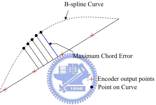
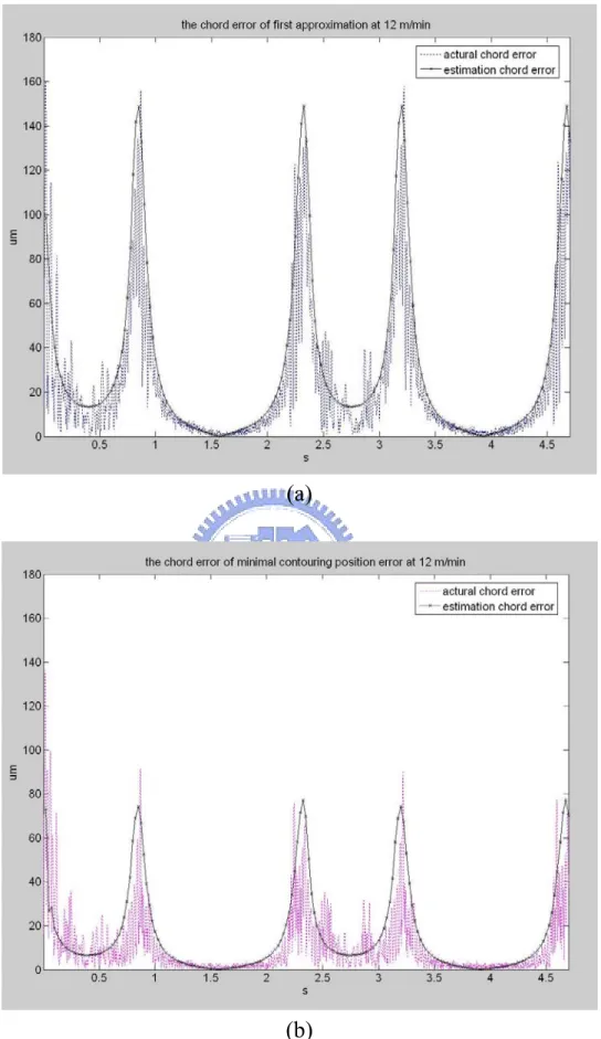
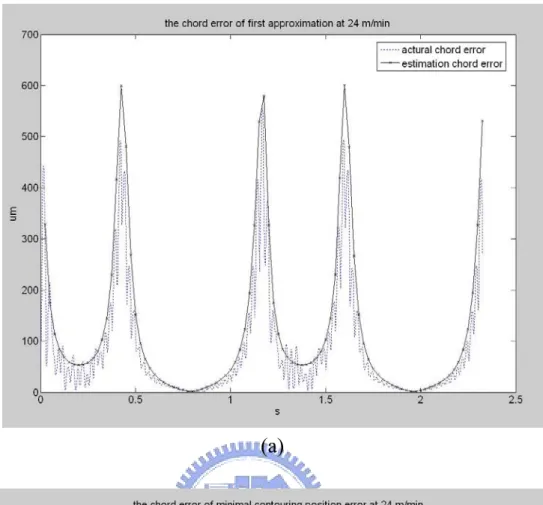
We want to find the chord error to verify the algorithm. An approximated method [20] is applied to estimate the chord error from data of experimental results. Using uniform interval interpolation with smaller ∆u to generate the curve data. Projection the curve data on the motor moving path, as shown Fig.5.7. If projection is out of the moving path segment, projection on the next moving segment. By doing so, it can be found several distance between the curve and the moving segment. Therefore, choosing the maximum distance is the chord error of the segment. The Fig.5.8(a) shows the chord error at 12 m/min using the first approximation interpolation, and Fig.5.8(b) shows the chord error using the minimal contouring position error interpolation. The Fig.5.9(a)(b) is the chord error at 24 m/min. observing the Fig5.8(a)(b) and 5.9(a)(b), it can be found that the chord error of the proposed algorithm is really less than the first approximation interpolation.

Chapter 6 Conclusion

For parametric curves, the contouring position error in terms of position is mainly determined by the radial error and the chord error. With the computer becomes much powerful, it is usually achieved very small radial error that can be ignored. For the reason, the chord error is the main concern in general interpolation algorithm. The proposed interpolation achieves better machining precision by considering minimization of the contouring position error. The simulation as well as the experimental results show that the proposed interpolation algorithm effectively improves the interpolation accuracy in terms of the contouring position error and maintains speed accuracy at the specified level.

Reference

[1] M Shpitalni, Y Koren, C C Lo “Realtime curve interpolators”, Computer -Aided Design, 26(11), pp.832-838, November 1994.

[2] P J Hartley, CJ Judd, “Parametrization and shape of B-spline curves for CAD”, Computer-Aided Design, 12(5), pp.235-238, September 1980.

[3] Bedi S, Ali I, Quan N, “Advanced Interpolation Techniques for N.C. Machines”, Transactions of the ASME. journal of engineering for industry, 115, pp329-336, August 1993.

[4] Yang DCH, Chou Jui-Jen, “Command Generation for Three-Axis CNC Machining”, Transactions of the ASME. journal of engineering for industry, 113, pp.305-310, August 1991.

[5] Jung-Tang Huang, Yang DCH, “A Generalized Interpolator for command generation of parametric curves in computer-controlled machines”, Japan/USA Symposium on Flexible Automation 1992, 1, pp.393-399.

[6] Yang DCH, Kong T, “Parametric interpolator versus linear interpolator for precision CNC machining”, Computer-Aided Design, 26(3), pp.225-233, March 1994.

[7] C C Lo, C Y Chung, “Curve Generation and Control for Biaxial Machine Tools”, J. CSME, 18(2), pp175-182, 1997.

[8] S S Yeh, P L Hsu, “The speed-controlled interpolator for machining parametric curves”, Computer-Aided Design, 31(5), pp.349-357, April 1999. [9] S S Yeh, P L Hsu, “Adaptive-feedrate interpolation for parametric curves

with a confined chord error”, Computer-Aided Design, 34(3), pp.229-237, March 2002.

[10] Tsehaw Tong, Ranga Narayanaswami, “A parametric interpolator with confined chord errors, acceleration and deceleration for NC machining”, Computer-Aided Design, 35(13), pp.1249-1259, November 2003.

[11] Rida T. Farouki, Yi-Feng Tsai, “Exact Taylor series coefficients for

variable-feedrate CNC curve interpolators”, Computer-Aided Design, 33(2), pp.155-165, February 2001.

[12] Richard J Sharpe, Richard W Thorne, “Numerical method for extracting an arc length parameterization from parametric curves”, Computer-Aided Design, 14(2), pp.79-81, March 1982.

[13] Brian Guenter, Richard Pareent, “Motion Control: Computing the Arc Length of Parametric Curves”, IEEE Computer Graphics and Applications, 10, pp.72-78, May 1990.

[14] John A. Roulier, Bruce Piper, “Prescribing the length of parametric curves”, Computer Aided Geometric Design, 13(1996), pp.3-22.

[15] Hans B. Kief, T. Frederick Waters, Computer Numerical Control, McGraw-Hill, 1992.

[16] lber G, Kim MS, Lee IK. “Comparing offset curve approximation methods”, IEEE Computer Graphics and Applications, 17(1997), pp.62-71.

[17] Elain Cohen, Richard F. Riesenfeld, Gershon Elber, Geometric Modeling with Splines: An Introduction, A K Peters, 2001.

[18] Nicholson, W. Keith, Elementary linear algebra,McGraw-Hill, 2001.

[19] Yoram Koren, Computer Control of Manufacturing Systems, McGraw-Hill, 1983.

[20] 廖家賢,「NURBS 插值器在 PC-BASED CNC 之設計與實現」國立中 央大學,碩士論文,民國 91 年

Figures

Curve

Segmentation Part Program

Curve Representation CAD Model Curve CAD Linear/Circular Real-Time Interpolator Control Loops CNC Machine Tool Reference points Line/Arc Segments (a) Part Program Curve Representation CAD Model CAD Linear/Circular/Curve Real-Time Interpolator Control Loops CNC Machine Tool Reference points Line/Arc/Curve Segments (b)

Fig.1.1 (a) Conventional method for machining curves (b) Currently more

(a)

(b)

Fig.2.3 (a) reference-pulse system and (b) sampled-data system.

(a)

(b)

Fig.2.5 Linear interpolation.

Fig.2.6 Circular interpolation.

(a) (b)

Fig.2.7 (a) Error in linear interpolation and (b) error in circular interpolation,

where Pref is the reference and P is the arrived point, e is the tracking error, and ε

Fig.2.8 Estimation of the next interpolated point. C(u) Parametric curve K(u) P(ui) Cutter path

ε

i P(ui+1)

Fig.3.1 Constant speed parametric curve interpolation.

Interpolation point Parametric curve Cutter path 1 Chord error (a) Chord error δ’ Cutter path 1 Radial error ε (b)

ε

i+1 Parametric curve

δ

'i Cutter path C(ui) C(ui+1) Circle K(ui) P(ui) P(ui+1) K(ui+1)

ε

i ) 2 (ui +ui+1 C ) 2 (ui+ui+1 K A(ui)

δ

i

Parametric curve Cutter path circle K(ui) P(ui) P(ui+1) K(ui+1) εi εi+1 ) 2 (ui+ui+1 K ) 2 (ui+ui+1 O δi δ'i θ θ (a) circle P(ui) P(ui+1) ) 2 (ui +ui+1 O θ δ''i εi+1 φ φ / 2 δ'i P'(ui+1) εi εi (b)

Fig.3.6. Verification Examples (a) perfect circle approximation and (b) mismatched radial errors.

-0.025 -0.02 -0.015 -0.01 -0.005 0 0.005 1 2 3 4 5 6 7 8 9 10 11 Eqn.(3-10) Eqn.(3-16)

-5

0 5

ε

i+1

θ

i

degree

Fig.3.7. Comparison of εi+1 evaluations.

-0.025 -0.02 -0.015 -0.01 -0.005 0 0.005 1 2 3 4 5 6 7 8 9 10 11 Eqn.(3-10) Eqn.(3-16)

-5

0 5

ε

i+1

θ

i

degree

Fig.4.1. The flowchart of program.

(a)

(b)

Fig.4.3. The chord errors of simulation results at 12 m/min (a) without adaptive feedrate (b) with adaptive feedrate.

(a)

(b)

Fig.4.4. The speed profile of simulation results at 12 m/min (a) without adaptive feedrate (b) with adaptive feedrate.

(a)

(b)

Fig.4.5. The Acceleration profile of simulation results at 12 m/min (a) without adaptive feedrate (b) with adaptive feedrate.

(a)

(b)

Fig.4.6. The chord errors of simulation results at 24 m/min (a) without adaptive feedrate (b) with adaptive feedrate.

(a)

(b)

Fig.4.7. The speed profile of simulation results at 24 m/min (a) without adaptive feedrate (b) with adaptive feedrate.

(a)

(b)

Fig.4.8. The Acceleration profile of simulation results at 24 m/min (a) without adaptive feedrate (b) with adaptive feedrate.

(a)

(b)

Fig.4.9. The chord errors of simulation results at 48 m/min (a) without adaptive feedrate (b) with adaptive feedrate.

(a)

(b)

Fig.4.10. The speed profile of simulation results at 4824 m/min (a) without adaptive feedrate (b) with adaptive feedrate.

(a)

(b)

Fig.4.11. The Acceleration profile of simulation results at 48 m/min (a) without adaptive feedrate (b) with adaptive feedrate.

Fig.5.1. The hardware layout of the experiment.

(a)

(b)

Fig.5.3. The encoder speed of experimental results at 12 m/min (a) without adaptive feedrate (b) with adaptive feedrate.

(a) Speed(speed 24m/min,freq=40Hz) 0 5 10 15 20 25 30 0 0.5 1 1.5 2 2.5 3 3.5 s m/min 4 AD Mout ADMCPE Mout (b)

Fig.5.4. The encoder speed of experimental results at 24 m/min (a) without adaptive feedrate (b) with adaptive feedrate.

(a)

(b)

Fig.5.5. The encoder speed of experimental results at 48 m/min (a) without adaptive feedrate (b) with adaptive feedrate.

(a) 120000 125000 130000 135000 140000 145000 150000 155000 160000 200000 210000 220000 230000 240000 250000 260000 first app. Pin first app. Mout MCPE Pin MCPE Mout curve

(b)

Fig.5.6. The encoder position of experimental results at 48 m/min (a) first approximation interpolation and minimal contour position error interpolation (b) the detail region.

Fig 5.7 Chord error estimation

Encoder output points B-spline Curve

Maximum Chord Error

(a)

(b)

Fig 5.8 Chord error estimation at 12 m/min (a) first approximation interpolation (b) minimal contour position error interpolation

(a)

(b)

Fig 5.9 Chord error estimation at 24 m/min (a) first approximation interpolation (b) minimal contour position error interpolation

Tables

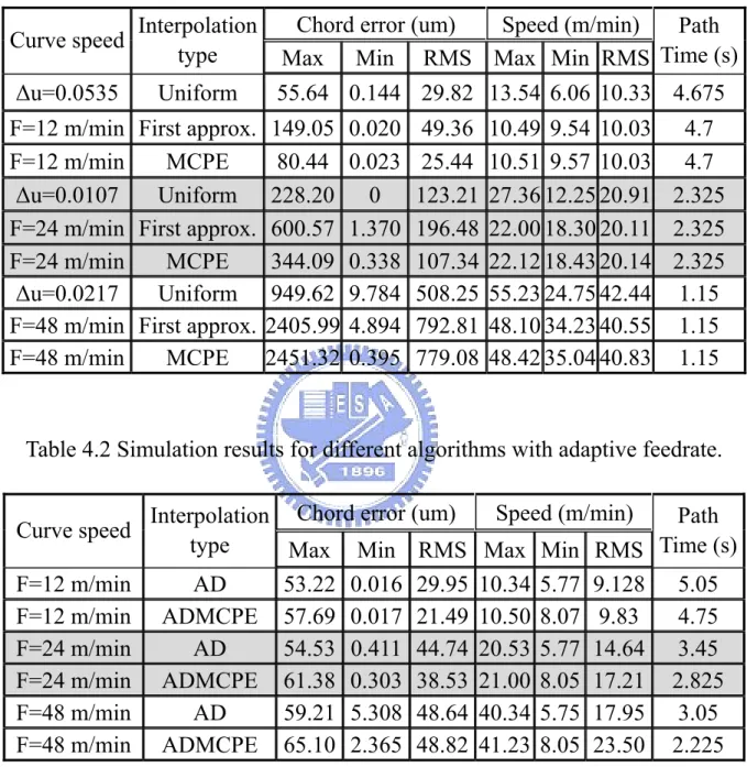
Table 4.1 Simulation results for different algorithms.

Chord error (um) Speed (m/min)

Curve speed Interpolation

type _{Max Min RMS Max Min RMS}

Path Time (s) ∆u=0.0535 Uniform 55.64 0.144 29.82 13.54 6.06 10.33 4.675 F=12 m/min First approx. 149.05 0.020 49.36 10.49 9.54 10.03 4.7

F=12 m/min MCPE 80.44 0.023 25.44 10.51 9.57 10.03 4.7

∆u=0.0107 Uniform 228.20 0 123.21 27.36 12.25 20.91 2.325

F=24 m/min First approx. 600.57 1.370 196.48 22.00 18.30 20.11 2.325

F=24 m/min MCPE 344.09 0.338 107.34 22.12 18.43 20.14 2.325

∆u=0.0217 Uniform 949.62 9.784 508.25 55.23 24.75 42.44 1.15 F=48 m/min First approx. 2405.99 4.894 792.81 48.10 34.23 40.55 1.15

F=48 m/min MCPE 2451.32 0.395 779.08 48.42 35.04 40.83 1.15

Table 4.2 Simulation results for different algorithms with adaptive feedrate.

Chord error (um) Speed (m/min)

Curve speed Interpolation

type _{Max Min RMS Max Min RMS}

Path Time (s) F=12 m/min AD 53.22 0.016 29.95 10.34 5.77 9.128 5.05 F=12 m/min ADMCPE 57.69 0.017 21.49 10.50 8.07 9.83 4.75 F=24 m/min AD 54.53 0.411 44.74 20.53 5.77 14.64 3.45 F=24 m/min ADMCPE 61.38 0.303 38.53 21.00 8.05 17.21 2.825 F=48 m/min AD 59.21 5.308 48.64 40.34 5.75 17.95 3.05 F=48 m/min ADMCPE 65.10 2.365 48.82 41.23 8.05 23.50 2.225

Table 4.3 Simulation results of computer time for different algorithms.

uniform First approx. MCPE AD ADMCPE