一維波方程系統中的等向與非等向混沌震動

國立交通大學應用數學系

博 士 論 文

一維波方程系統中的等向與非等向混沌震動

Isotropic and Nonisotropic Chaotic Vibrations

of the 1D Wave System

研 究 生：胡忠澤

指導教授：林文偉 教授

一維波方程系統中的等向與非等向混沌震動

Isotropic and Nonisotropic Chaotic Vibrations

of the 1D Wave System

研 究 生：胡忠澤 Student：Chung-Che Hu

指導教授：林文偉 Advisor：Wen-Wei Lin

國 立 交 通 大 學

應 用 數 學 系

博 士 論 文

A Thesis

Submitted to Department of Applied Mathematics

National Chiao Tung University

in partial Fulfillment of the Requirements

for the Degree of

Doctor of Philosophy

in

Applied Mathematics

June 2009

Hsinchu, Taiwan, Republic of China

一維波方程系統中的等向與非等向混沌震動

研 究 生：胡忠澤 指導教授：林文偉

國 立 交 通 大 學

應 用 數 學 系

摘要

波方程在一維閉區間 I 的右端有梵德波形式的非線性邊界條件。而在

閉區間 I 的左端，當參數

η

>

0

時其邊界條件為能量的輸入；當

η

=

0

時

其邊界條件為齊次諾曼條件。這個波方程系統的解與一個區間函數的

疊代有關，所以我們定義當這個區間函數有李—約克的渾沌現象時稱

這個波方程系統有混沌震動。因為在我們討論的波方程系統中兩特徵

線的運動速度為任意兩正數 與 ，所以系統中有著等向性與非等向

性的混沌震動現象產生。在這篇論文中，我們將討論波方程系統中混

沌震動現象的產生分別與參數

c

c

η

、 、 變化之間的關聯。

c

c

Isotropic and Nonisotropic Chaotic

Vibrations of the 1D Wave System

Student : Chung-Che Hu

Advisor : Wen-Wei Lin

Department of Applied Mathematics

National Chiao Tung University

Abstract

A wave equation on a one-dimensional interval I has a van der Pol type nonlinear boundary condition at the right end. At the left end, the boundary condition is energy-injecting if the

parameter > 0 and is the homogeneous Neumann condition if

= 0. The solution of the wave system is corresponding to the iteration of one interval map, so we say the wave system is chaotic if the interval map is chaotic in the sense of Li-Yorke. The sys-tem which we consider contains both isotropic and nonisotropic chaotic vibrations, since the two associated families of character-istics travel with two speeds c1, c2 for any given positive c1, c2. In

this paper, we discuss that the chaotic vibrations of the 1D wave

誌 謝

僅以此論文，獻給最疼愛我的爺爺—胡大洲先生

從中研院數學所研究助理、清大數學碩士、交大應用數

學博士這七年的歲月，我前後跟著台灣數學界最具引響力的

三位數學家學習到一個研究者應有的態度—充分利用時間

並且努力做到最好。在中研院兩年的時間，李國偉教授教我

許多做人處事的道理，我在李老師的身上看到高尚的人格，

李老師眼睛看到的都是別人的優點，他熱心幫忙協助他身邊

所有需要幫助的的人，所以李老師的身邊總是有許多受到他

鼓舞的年輕人，而我就是其中的一個。很難相信一位像李老

師這樣有名的數學家，會願意花時間在一個大學剛畢業，甚

麼都不懂的我身上，耐心的指導我數學觀念，也是從那時候

開始，我才漸漸知道數學是甚麼，也對數學產生興趣。

清華大學碩士班指導教授王懷權老師在我心目中就像

是我的親人一樣，從準備博士班考試一直到博士班畢業，他

不斷的在我最需要的時候給予我最大的幫助，在碩士班受他

指導時，最常聽王老師說到他讀書時一大早起床為了比其他

同學多讀一些書的故事，也是這樣努力才讓王老師有今日如

此不凡的成就。

交通大學博士班指導教授林文偉老師就像是一個充滿

俠義心腸的劍客一樣，在我人生最絕望的時候，願意伸出他

的手幫助我，這一年來在星期五論文研討時，聽到老師對我

們的叮嚀—要每秒鐘都要想數學才有機會做到別人所不能

的問題，他也有著極大的耐心來指導每一位學生。在這三位

老師身上，我看到了身為數學家的風範，也看到我將來人生

最佳的模範。

另外，也感謝這一路上幫助過我的交通大學數學系與師

培中心的老師們，交通大學是一個充滿關懷與愛的學校，很

榮幸能在這度過五年的時光。也很感謝身邊的同學們，其

儒、明杰與文貴，在我最需要的時候都有你們在身邊讓我感

到溫暖，謝謝你們。

最後要感謝我的父母、岳母、文琪跟忠洪，在我的人生

中你們給予我太多，不管是任何我需要的方面，你們都支持

著我，謝謝你們。而我摯愛的太太雯玲與女兒勻馨，你們陪

我走過人生中最難熬的歲月，也因為你們的陪伴，我才有走

下去的勇氣，每次回到家看到你們就覺得生命是無價的，也

有更大的勇氣跟力量面對一切的考驗。

主阿!

感謝你對我禱告的垂聽，希望你能照顧我在天國的長

輩，爺爺與雯玲的外婆，感謝主。

Contents

Abstract (in Chinese)

i

Abstract (in English)

ii

Acknowledgements iii

Contents vi

1 Introduction

1

2 Preliminary

7

3 The 1D wave system (1.1)-(1.4)

11

3.1 Chaotic vibrations of the system (1.1)-(1.4)…...

11

3.2 The chaotic region of the system (1.1)-(1.4)... 14

3.3 Main results of the system (1.1)-(1.4)……… 22

4 The 1D wave system (1.12)

27

4.1 Chaotic vibrations of the system (1.12)………. 27

4.2 The chaotic region of the system (1.12)………. 30

4.3 Main results of the system (1.12)………... 41

5 Three

examples

45

5.1 One special case of the system (1.12)……… 45

5.2 Main results of the system (1.5)-(1.7)……… 51

5.3 Main results of the system (1.8)-(1.11)……….. 55

6 Two methods to detect chaos 60

6.1 Chaos in the 1D wave systems (1.1)-(1.4) and (1.12)…… 61

6.2 Further discussions………. 69

Chapter 1

Introduction

The imbalance of the boundary energy ‡ow due to energy injection at one end and a nonlin-ear van der Pol boundary condition at the other end of the spatial one-dimensional interval can cause isotropic chaotic vibration of the linear wave equation. Such chaotic vibration is isotropic with respect to space and time because the two associated families of characteristics both propagate with the same speed (see Chen et al. [2]). In [2], the 1D wave system is considered:

!tt !xx = 0, 0 < x < 1, t > 0,

with the boundary conditions 8 > > > < > > > : !t(0; t) = !x(0; t), > 0, 6= 1, t > 0, !x(1; t) = !t(1; t) !3t(1; t), 2 (0; 1], > 0, t > 0,

and the initial conditions

!(x; 0) = '(x) 2 C1([0; 1]), !t(x; 0) = (x) 2 C0([0; 1]).

In the 1D wave equation !tt !xx = 0, two families of characteristics travel with the same speed

c1 = c2 = 1. The boundary condition at the left endpoint x = 0 is energy-injecting and the

1D wave system is chaotic when the parameter enters the region " 3p3 1 3p3 + 1 + ; 1 ! [ 1;3 p 3 + 1 + 3p3 1 #

, for any given _{2 (0; 1],} > 0.

In [8, 12, 13], the 1D wave system is considered:

!tt !xx = 0, 0 < x < 1, t > 0,

with the boundary conditions 8 > > > < > > > : !x(0; t) = !t(0; t), > 0, 6= 1, t > 0, !x(1; t) = !t(1; t) !3t(1; t), 2 (0; 1], > 0, t > 0,

and the initial conditions

!(x; 0) = '(x) 2 C1([0; 1]), !t(x; 0) = (x) 2 C0([0; 1]).

Huang et al. characterized the dynamical behavior in terms of the growth of the total variation of

the interval map and proved that for any given _{2 (0; 1], there exist four constants 0}, _H, _H

and ₀ with

0 < ₀< _H < 1 < _H < _{0< 1}

such that the total variation of the interval map remains bounded, is unbounded, is unbounded

exponentially when the parameter belongs to (0; _{0)[( 0; 1), ( 0}; _{H)[( H}; ₀), and ( _{H; 1)[}

(1; _H), respectively. In particular, the last case corresponds to chaos in the 1D wave system.

No-tice that the boundary condition at the left endpoint in this system is !x(0; t) = !t(0; t) which

is di¤erent from !t(0; t) = !x(0; t) in [2].

By including a mixed partial derivative linear transport term in the wave equation, nonlinear-ity in the van der Pol boundary condition can also cause nonisotropic chaotic vibration (without energy injection from the other end). Such chaotic vibration is nonisotropic with respect to space

which satisfy c1c2 = 1 (see Chen et al. [5]). In [5], the 1D wave system is considered:

!tt+ v!tx !xx = 0, v > 0, 0 < x < 1, t > 0,

with the boundary conditions

!x(0; t) = 0, t > 0, and !x(1; t) = !t(1; t) !3t(1; t), 2 0; v +pv2_{+ 4} 2 # , > 0, t > 0, and the initial conditions

!(x; 0) = '(x) 2 C1([0; 1]), !t(x; 0) = (x) 2 C0([0; 1]).

In the 1D wave equation !tt+v!tx !xx = 0, two families of characteristics travel with di¤erent

speeds c1 = v+

p v2₊₄

2 and c2 =

v+pv2₊₄

2 which satisfy c1c2 = 1 and c2 c1 = v. The boundary

condition at the left endpoint x = 0 is the homogeneous Neumann condition and the boundary condition at the right endpoint x = 1 is a van der Pol condition. In [5], Chen et al. proved the 1D wave system is chaotic when the parameters (v; ) enter a certain subregion of

S = ( (v; ) 2 R2 j 0 < v < 1; 0 < v + p v2_{+ 4} 2 ) .

In [9], Huang proved that there exist three subregions S0

1, S11 and S2of S such that the growth of

the total variation of the interval map remains bounded, is unbounded, is unbounded exponentially

when the parameters (v; ) belong to S0

1, S11, and S2, respectively. In particular, the last case

cor-responds to chaos in the 1D wave system.

In chapter 3 of this paper, the 1D wave system is considered:

!tt d!tx c2!xx = 0, d 2 R, c > 0, 0 < x < 1, t > 0, (1.1)

with the boundary conditions

!x(0; t) = !t(0; t), 0, 6=

1 c2

and

!x(1; t) = !t(1; t) !3t(1; t), 2 0;

1 c1

, > 0, t > 0. (1.3)

And with the initial conditions

!(x; 0) = '(x) 2 C1([0; 1]), !t(x; 0) = (x) 2 C0([0; 1]). (1.4)

Remark 1.0.1 We denote the parameters

c1= d +pd2_{+ 4c}2 2 and c2 = d +pd2_{+ 4c}2 2 in (1.2) and (1.3).

In the 1D wave equation !tt d!tx c2!xx = 0, two families of characteristics travel with

speeds c1 and c2. If d = 0, the speeds c1 = c2 = c; if d 6= 0, the speeds c1 6= c2. The

bound-ary condition at the left endpoint x = 0 is energy-injecting when > 0 and is the homogeneous

Neumann condition when = 0. The boundary condition at the right endpoint x = 1 is a van

der Pol condition which is a well-known self-regulating mechanism in automatic control.

If d = 0, c2 = 1 in (1.1) and > 0 in (1.2), we have the 1D wave equation

!tt !xx = 0, 0 < x < 1, t > 0, (1.5)

with the boundary conditions 8 > > > < > > > : !x(0; t) = !t(0; t), > 0, 6= 1, t > 0, !x(1; t) = !t(1; t) !3t(1; t), 2 (0; 1], > 0, t > 0, (1.6)

and the initial conditions

!(x; 0) = '(x) 2 C1([0; 1]), !t(x; 0) = (x) 2 C0([0; 1]). (1.7)

If d = v, c2 _{= 1 in (1.1) and = 0 in (1.2), we have the 1D wave equation}

with the boundary conditions !x(0; t) = 0, t > 0, (1.9) and !x(1; t) = !t(1; t) !3t(1; t), 2 0; v +pv2_{+ 4} 2 # , > 0, t > 0, (1.10)

and the initial conditions

!(x; 0) = '(x) 2 C1([0; 1]), !t(x; 0) = (x) 2 C0([0; 1]). (1.11)

Thus, the 1D wave system (1.1)-(1.4) contains the 1D wave systems in [8, 12, 13] and [5, 9]. Fur-thermore, the system (1.1)-(1.4) contains both isotropic and nonisotropic chaotic vibrations since

the two associated families of characteristics travel with two speeds c1, c2 for any given positive

c1, c2. In section 3, we show the chaotic region of the 1D wave system. And based on this region,

we show the chaotic region of the paramerter when the other parameters are …xed. Furthermore,

we show the system is chaotic if c1 ! 1, or c1 ! 0+, or c2 ! 1.

In chapter 4, the 1D wave system is considered: 8 > > > > > > < > > > > > > : !tt d!tx c2!xx = 0, d 2 R, c > 0, 0 < x < 1, t > 0, !t(0; t) + !x(0; t) = 0, > 0, 6= c2, t > 0, !x(1; t) = !t(1; t) !2m+1t (1; t), 2 0;c11 i , ; t > 0, m 2 N, !(x; 0) = '(x) 2 C1([0; 1]), !t(x; 0) = (x) 2 C0([0; 1]). (1.12)

In this system, the boundary condition at the left endpoint x = 0 is energy-injecting and the bound-ary condition at the right endpoint x = 1 has odd-degree nonlinearity. In section 4, we show the

1D wave system (1.12) is chaotic when the parameter satis…es either

c2 < c2 2mc1(1 + c2) + 2m p 2m + 1(2m + 1)(c1+ c2) 2mp 2m + 1(2m + 1)(c1+ c2) 2mc2(1 + c2) or c2 2mp2m + 1(2m + 1)(c1+ c2) 2mc1(1 + c2) 2mc2(1 + c2) + 2mp2m + 1(2m + 1)(c1+ c2) < c2

for any given parameters c, d, , , m satisfy inequality

2mp

and when the parameter satis…es either > c2 or c2 2m p 2m + 1(2m + 1)(c1+ c2) 2mc1(1 + c2) 2mc2(1 + c2) + 2mp2m + 1(2m + 1)(c1+ c2) < c2

for any given parameters c, d, , , m satisfy the inequality

2mp

2m + 1(2m + 1)(c1+ c2) 2mc2(1 + c2) 0.

And we show the 1D wave system (1.12) is chaotic for any given c1 if the parameters , c2, , ,

m satisfy

> c2 and 2mc2(1 + c2) 2m

p

2m + 1(2m + 1)( c2) 0.

And the 1D wave system (1.12) is chaotic for su¢ ciently small c1if the parameters , c2, , , m

satisfy some conditions or c1 is su¢ ciently large if the parameters , c2, , , m satisfy some other

conditions.

It is easy to see that the 1D wave system (1.12) contains the 1D wave system in [2]. Thus, we consider the 1D wave systems in [2, 5, 8, 9, 12, 13] as three examples of the systems (1.1)-(1.4) and (1.12) in chapter 5. And in chapter 6, we use two methods to detect the chaos in 1D wave systems (1.1)-(1.4) and (1.12) (see Li et al. [14, 15]).

Chapter 2

Preliminary

We list some de…nitions and background facts that a reader should know in this chapter.

De…nition 2.0.2 (Topologically Transitive) _{A map f : X ! X is (topologically) transitive}

on an invariant set Y provided the forward orbit of some point p is dense in Y . The Birkho¤ Tran-sitivity Theorem proves that a map f is transitive on Y if and only if, given any pair of open sets

U , V Y there exists k > 0 such that fk_{(U ) \ V 6= ?.}

Intuitively, a topologically transitive map has points which eventually move under iteration from one arbitrarily small neighborhood to any other. Consequently, the dynamical system cannot be decomposed into two disjoint open sets which are invariant under the map.

De…nition 2.0.3 (Sensitive Dependence on Initial Conditions) _{A map f : X ! X has}

sensitive dependence on initial conditions if there exists > 0 (independent of the point) such that,

for each point x 2 X and any neighborhood N of x, there exists y 2 N such that d (fn(x); fn(y))

for some n 0 .

Intuitively, a map possesses sensitive dependence on initial conditions if there exist points

ar-bitrarily close to x which eventually separate from x by at least under iteration of f . We

empha-size that not all points near x need eventually separate from x under iteration, but there must be at least one such point in every neighborhood of x.

De…nition 2.0.4 (Expansive) A map f on a metric space X is said to be expansive provided there

is an r > 0 (independent of the point) such that, for each pair of points x; y 2 X there is a k 0

If f is expansive and X is a perfect metric space, then it has sensitive dependence on initial conditions.

De…nition 2.0.5 (Chaotic in the Sense of Devaney) _{Let V be a set. f : V ! V is said to be}

chaotic on V if

1. f has sensitive dependence on initial conditions. 2. f is topologically transitive.

3. periodic points are dense in V .

De…nition 2.0.6 (Chaotic in the Sense of Robinson) A map f on a metric space X is said

to be chaotic on an invariant set Y or exhibits chaos provided (i) f is transitive on Y and (ii) f has sensitive dependence on initial conditions on Y .

The paper of Banks, Brooks, Cairns, Davis, and Stacey (1992) proves that any map which (i) is transitive on Y and (ii) has dense periodic points also must have sensitive dependence on ini-tial conditions.

De…nition 2.0.7 (Chaotic in the Sense of Li-Yorke) A continuous map f on the compact

met-ric space (X; d) is said to be chaotic on a nonempty and invariant set X0in the sense of Li-Yorke

if there is an uncountable set S X0 such that

(i) lim sup_n!1d(fn_{(x); f}n_{(y)) > 0, for all x, y 2 S and x 6= y.}

(ii) lim inf_n!1d(fn(x); fn_{(y)) = 0, for all x, y 2 S.}

Theorem 2.0.8 _{[17, Li and Yorke, 1975]Assume f : R ! R is continuous, and there is a point}

a such that either (i) f3(a) a < f (a) < f2(a) or (ii) f3(a) a > f (a) > f2(a). Then, f has points of all periods.

De…nition 2.0.9 In order to state the result of Sharkovskii, we need to introduce a new ordering

on the positive integers using the symbolB, called the Sharkovskii ordering.First, the odd integers

greater than one are put in the backward order:

3B 5 B 7 B 9 B 11 .

odd integers times increasing powers of two:

3B 5 B 7 B B 2 3 B 2 5 B 2 7 B B 22 3B 22 5B 22 7B

B 2n _{3B 2}n _{5B 2}n _{7B B 2}n+1 _{3B 2}n+1 _{5B 2}n+1 _{7B .}

Finally, all the powers of two are added to the ordering in decreasing powers:

3B 5 B B 2n 3B 2n 5B B B 2n+1B 2nB B 22 B 2 B 1.

We have now given an ordering between all positive integers. This ordering seems strange but it turns out to the be ordering which expresses which periods imply which other periods as given in the the-orem of Sharkovskii (Sharkovskii, 1964).

Theorem 2.0.10 (Sharkovskii) Let f : I _{R ! R be a continuous function from an interval}

I into the real line. Assume f has a point of period n and nB k. Then, f has a point of period k.

(By period, we mean least period.)

Theorem 2.0.11 (Period Doubling Bifurcation) _{Assume that f : R}2 _{! R is a C}r function

jointly in both variables with r 3, and that f satis…es the following conditions.

(1) The point x0 is a …xed point for = 0: f (x0; 0) = x0.

(2) The derivative of f ₀ at x0 is 1: f0₀(x0) = 1. Since this derivative is not equal to 1, there

is a curve of …xed points x( ) for near ₀.

(3) The derivative of f0_{(x( )) with respect to is nonzero (the derivative is varying along the}

fam-ily of …xed points):

= @ 2_f @ @x + 1 2 @f @ @2f @x2 (x0; 0) 6= 0. (4) The graph of f2

0 has nonzero cubic term in its tangency with the diagonal (the quadratic term

is zero): = 1 3! @3f @x3(x0; 0) + 1 2! @2f @x2(x0; 0) 2 6= 0.

Then, there is a period doubling bifurcation at (x0; 0). More speci…cally, there is a di¤ erentiable

curve of …xed points, x( ), passing through x0 at 0, and the stability of the …xed point changes at

0. (Which side of 0 is attracting depends on the sign of .) There is also a di¤ erentiable curve

is tangent to the line R f 0g at (x0; 0), so is the graph of a function of x, = m(x) with

m0_{(x0) = 0 and m}00_{(x0) = 2 = 6= 0. The stability type of the period 2 orbit depends on the}

sign of : if > 0, then the period 2 orbit is attracting; and if < 0, then the period 2 orbit is

repelling.

De…nition 2.0.12 (Homoclinic Point) _{Let a map f 2 C(I; I). A point x 2 I is called}

homo-clinic point of f if there exists a periodic point p of period n with x 6= p, x 2 Wu(p; fn) and fnm(x) =

p for some positive integer m. We call such point p a periodic point associated with a homoclinic

point x and denote by Ph(f ) the set of all such periodic points.

In [10, Corollary 9.1], Chen et al. proved the results as below.

Lemma 2.0.13 _{[10, Corollary 9.1]Let f 2 C(I; I). Suppose that f is piecewise monotone with}

…nitely many extremal points on I. Then the following conditions are equivalent. (1) f has a periodic point whose period is not a power of 2.

(2) f has a homoclinic point. That is, Ph(f ) 6= ?.

(3) f has positive topological entropy.

(4) The total variation VI(fn) of f on I grows exponentially as n ! 1.

Furthermore, each of the above conditions implies that f is chaotic in the sense of Li-Yorke.

Remark 2.0.14 In [10, Corollary 9.1], Chen et al. have the conclutions as below.

If f is piecewise monotone with …nitely many extremal points on I, then

Chaos in the sense of Devaney)sensitive dependence on initial conditions)exponential grows of

the total variation VI(fn) with respect to n as n ! 1 )positive topological entropy,existence

of a periodic point of a period being not a power of 2 ,existence of a homoclinic point,Chaos in the sense of Li-Yorke.

Chapter 3

The 1D wave system (1.1)-(1.4)

!tt d!tx c2!xx = 0, d 2 R, c > 0, 0 < x < 1, t > 0,

with the boundary conditions

!x(0; t) = !t(0; t), 0, 6= 1 c2 , t > 0, and !x(1; t) = !t(1; t) !3t(1; t), 2 0; 1 c1 , > 0, t > 0. And with the initial conditions

!(x; 0) = '(x) 2 C1([0; 1]), !t(x; 0) = (x) 2 C0([0; 1]).

3.1

Chaotic vibrations of the system (1.1)-(1.4)

The general solution of (1.1) is

where u, v are arbitrary C2-function. Substituting (3.1) in (1.2) and (1.3), we have u0(c1t) = 1 c2 1 + c1 v0(c2t), t > 0, (3.2) and (c1u0(c1t + 1) + c2v0(c2t 1))3+ _c1₁ (c1u0(c1t + 1) + c2v0(c2t 1)) 1 +c2 c1 v 0_{(c2t 1) = 0, t > 0.} (3.3) When = _c1 2 in (3.2), we have

u0(c1t) = 0 for t > 0 ) u(c1t + x) = C for t > 0.

Thus, we consider the case _{6= c}1

2. And depends on (3.2), we can use v

0 _{to replace u}0 _{in (3.3) to}

derive one di¤erence equation as follows. By using the substitution

z(c1t) = 8 > > > < > > > : v0(c2t 1) , 0 t _c1₂, 1+ c1 1 c2u 0 _c 1t c_c1₂ , t > _c1₂,

we have the di¤erence equation

c11_{1+ c}c2₁z( + ) + c2z( ) 3 + _c1 1 c1 1 c2 1+ c1z( + )+ c2z( ) 1 +c_c2₁ z( ) = 0, (3.4) where = c1t, = 1 +c_c1₂.

And the initial condition of (3.4) is

z(c1t) = 8 > > > > < > > > > : (1 c2t) c1'0(1 c2t) c1+c2 , 0 t 1 c2. 1+ c1 1 c2 c1t c1_c2 +c2'0 c1t c1_c2 c1+c2 , 1 c2 < t 1 c1 + 1 c2.

z( ) is continuous onh0; 1 + c1

c2

i

and satis…es the compatibility condition

c11_{1+ c}c2₁z( ) + c2z(0) 3 + _c1 1 c1 1 c2 1+ c1z( ) + c2z(0) 1 +c2 c1 z(0) = 0.

De…nition 3.1.2 We denote the range of z( ) on [0; ] to be the compact interval ; i.e., =

z([0; ]).

We show the dependence of z( + ) on z( ) is given implicitly by one C1-function f as

fol-lows.

Lemma 3.1.3 (Existence and Uniqueness of the Solution) Let the parameters c1, c2, , ,

be …xed in (3.4) with c1 > 0, c2 > 0, 0, 6= _c1₂, 2 0;_c1₁

i

and > 0. Then there exists

one C1-function f such that

f (z(t)) = z(t + ) for all t > 0, where = (c1; c2; ; ; ). Proof.Let H (u; v) = c11_{1+ c}c2₁u + c2v 3 + _c1 1 c1 1 c2 1+ c1u + c2v 1 +c2 c1 v = 0, where u = z( + ), v = z( ), = (c1; c2; ; ; ). (i) If = _c1

1, then H (u; v) = 0 implies

c1 1 c2 1 + c1 u = s 1 +c2 c1 v c2v.

Hence, the C1-function f exists.

(ii) If _{2 0;c}1 1 , then @ @uH (u; v) = 3 c1 1 c2 1 + c1 c1 1 c2 1 + c1 u + c2v 2 + (1 c1) 1 c2 1 + c1 6= 0.

By the implicit function theorem, the C1-function f exists.

De…nition 3.1.4 We denote f (z( )) = z( + ) to be the function, which satis…es (3.4) for all

0, where = ( ; c1; c2; ; ).

Since

f (z( )) = z( + ) for all > 0,

we can use the map f and the interval to generate z( ) for all > 0. And the corresponding

solution of the 1D wave system (1.1)-(1.4) is calculated via the formulae

!(x; t) = Z t+x c1+ 1 c2 1 c2 c1 1 c2 1 + c1 z(c1 )d + Z t x c2+ 1 c2 0 c2z(c1 )d .

De…nition 3.1.5 (Chaotic Vibration) The solution of the 1D wave system is said to be chaotic

if the map f : _{! R is chaotic in the sense of Li-Yorke; i.e., there exists one nonempty}

invari-ant subset 0 such that f is chaotic in the sense of Li-Yorke on 0 (see De…nition 2.0.7).

Remark 3.1.6 In this paper, we say the 1D wave system is chaotic if its solution is chaotic.

3.2

The chaotic region of the system (1.1)-(1.4)

In this section, we want to show the chaotic region of the solution of the 1D wave system (1.1)-(1.4). First, we consider (3.4) as below:

H (x; y) = c11_{1+ c}c2₁y + c2x 3 + _c1 1 c1 1 c2 1+ c1y + c2x 1 + c2 c1 x = 0, where c1, c2 > 0, 0, 6= _c1₂, 2 0;_c1₁ i and > 0. De…nition 3.2.1 We denote vc = c1 2 c1c2+ 3c2 3c2(c1+ c2) r 1 + c2 3 c2 and M = 2(1 + c2)(1 + c1) 3(c1+ c2)(1 c2) r 1 + c2 3 c2

in the following lemmas.

We show the local maximum, minimum and piecewise monotonicity of the function f which satis…es (3.4) as below.

Lemma 3.2.2 (Local Maximum, Minimum and Piecewise Monotonicity) The function f

is odd and f has local extrema at (vc; M ) and ( vc; M ). Furthermore, f is strictly monotonic

on ( 1; vc), ( vc; vc) and (vc; 1).

Proof.Since H( x; f ( x)) = H( x; f (x)) = 0, we have f ( x) = f (x). Thus f is odd.

Then use d dxH(x; y) = 3 c1 1 c2 1+ c1y + c2x 2 c11_{1+ c}c2₁y0+ c2 + _c1 1 c1 1 c2 1+ c1y 0_{+ c2 1 +}c2 c1 = 0,

and carry out the computations, we have the results.

We show the x-axis Intercepts, …xed points and intersections with the line y = x of the

func-tion f as below.

Lemma 3.2.3 (x-axis Intercepts) The function f intersects the x-axis at the points 1 c2 r 1 + c2 c2 ; 0 , (0; 0), 1 c2 r 1 + c2 c2 ; 0 .

Proof.The results can be directly com…rmed by computing H(x; 0) = 0.

Lemma 3.2.4 (Intersections with the Line y = x) The function f intersects the line y = x

at the points 1 + c1 c1+ c2 r + ; 1 + c1 c1+ c2 r + , (0; 0) and 1 + c1 c1+ c2 r + ;1 + c1 c1+ c2 r + .

Proof.The results can be directly com…rmed by computing H(x; x) = 0.

De…nition 3.2.5 We denote the point

B = 1 + c1

j2 c1c2+ c2 c1j

s

2 + 2 c1c2+ (c1 c2) + (c2 c1)

(2 c1c2+ c2 c1)

in the following lemmas.

Lemma 3.2.6 (Intersections with the Line y = x) Let the parameters , c1, c2, , be …xed

in (3.4) with 2+2 c1c2+ (c1 c2)+ (c2 c1)

(2 c1c2+c2 c1) > 0, then the function f intersects the line y = x at

the points ( B; B), (0; 0), (B; B). Otherwise, the function f intersects the line y = x only at

Proof.The results can be directly com…rmed by computing H(x; x) = 0.

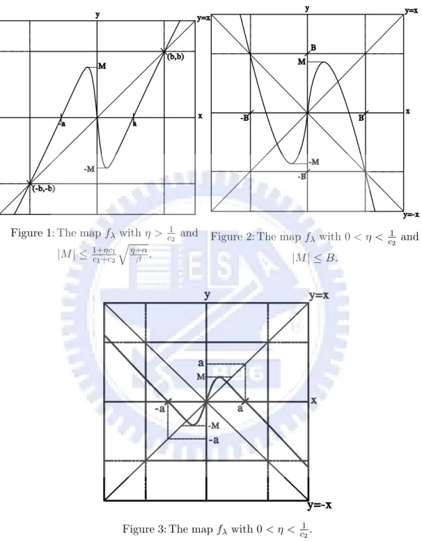
Figure 1: The map f with > _c1

2 and

jMj 1+ c1

c1+c2

q

+ _.

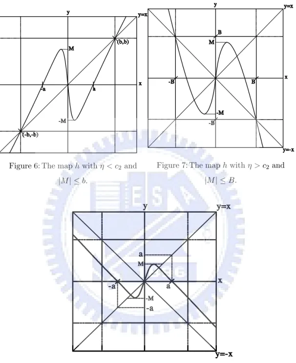
Figure 2: The map f with 0 < < _c1

2 and

jMj B.

Figure 3: The map f with 0 < < _c1

Figure 4: f3_(p

2) < p2< f (p2) < f2(p2). Figure 5: f6(p5) < p5< f2(p5) < f4(p5).

We show the function f has bounded invariant interval or bounded invariant cantor-like sub-set in following lemmas.

Lemma 3.2.7 (Bounded Invariant Interval) Let the parameters , c1, c2, , be …xed in (3.4).

(i) If > _c1 2 and jMj = 2(1+ c2)(1+ c1) 3(c1+c2)(1 c2) q 1+ c2 3 c2 1+ c1 c1+c2 q

+ _{, then the iterates of every point}

in the set U _1; 1 + c1 c1+ c2 r + [ 1 + c_c 1 1+ c2 r + ; 1

escape to _{1, while those of any point in RnU are attracted to the bounded invariant interval}

2(1 + c2)(1 + c1) 3(c1+ c2)(1 c2) r 1 + c2 3 c2 ; 2(1 + c2)(1 + c1) 3(c1+ c2)(1 c2) r 1 + c2 3 c2 of f , i.e., [ _{jMj ; jMj] of f .} (ii) If 0 < < _c1

2 and f intersects the line y = x at three points and jMj B, then the iterates

of every point in the set U _{( 1; B) [ (B; 1) escape to 1, while those of any point in RnU}

are attracted to the bounded invariant interval [ _{jMj ; jMj] of f .}

(iii) If 0 < < _c1

2 and f intersects the line y = x at (0; 0), then the iterates of every point in

R are attracted to the bounded invariant interval [ jMj ; jMj] of f .

Proof.The results of (i) and (ii) follow easily from the above lemmas and other piecewise monotonic

We omit the details. (iii) If 0 < < _c1

2 and f intersects the line y = x only at (0; 0), then jf (x)j < jxj for all

x 2 1; _c1 2 r 1 + c2 c2 [ 1 c2 r 1 + c2 c2 ; 1 .

Thus, jfn_{(x)j is strctly decreasing for n n}

0, where fn0 (x) 2 1; _c1 2 r 1 + c2 c2 [ 1 c2 r 1 + c2 c2 ; 1 and fn0+1_{(x) =} 2 1; _c1 2 r 1 + c2 c2 [ 1 c2 r 1 + c2 c2 ; 1 .

Hence, the iterates of every point in R are attracted to the bounded invariant interval [ jMj ; jMj] of f (see Figure 3).

Lemma 3.2.8 (Bounded Cantor-like Invariant Subset) The bounded invariant interval

2(1 + c2)(1 + c1) 3(c1+ c2)(1 c2) r 1 + c2 3 c2 ; 2(1 + c2)(1 + c1) 3(c1+ c2)(1 c2) r 1 + c2 3 c2

no longer exists in the case (i) and (ii) of the Lemma 3.2.7 if the condition

jMj 1 + c1

c1+ c2

r +

or jMj B

is violated. Instead, we have a bounded Cantor-like invariant set.

Proof.The method of proof is now standard, see [18, Sec. 1.7], for example.

We have the chaotic region of the function f as below.

Lemma 3.2.9 Let the parameters , c1, c2, , be …xed in (3.4) and satisfy the inequality

2(1 + c2)(1 + c1) 3(c1+ c2)(1 c2) r 1 + c2 3 c2 1 c2 r 1 + c2 c2 , (3.5)

then the interval map f is chaotic in the sense of Li-Yorke if the domain of f contains the inter-val 1 c2 r 1 + c2 c2 ; 1 c2 r 1 + c2 c2 .

Proof.(i) If 0 < < _c1 2, then f (vc) = 2(1 + c2)(1 + c1) 3(c1+ c2)(1 c2) r 1 + c2 3 c2

is the local maximum.

Since f is strictly increasing on [0; vc] and f (vc) _c1₂

q

1+ c2

c2 , there exists one unique point p12

(0; vc] such that f (p1) = _c1₂

q

1+ c2

c2 . Similarly, there exists one unique point p2 2 (0; p1) such

that f (p2) = p1. Hence, we have

0 = f3(p2) < p2 < f (p2) < f2(p2) (see Figure 4).

Thus, f has points of all periods which implies chaos [by Li and Yorke, 1975]. (ii) If > _c1 2, then f (vc) = 2(1 + c2)(1 + c1) 3(c1+ c2)(1 c2) r 1 + c2 3 c2

is the local minimum and

f ( vc) = 2(1 + c2)(1 + c1) 3(c1+ c2)(1 c2) r 1 + c2 3 c2

is the local maximum.

Since f is strictly decreasing on [ vc; vc] and f (vc) _c1₂

q

1+ c2

c2 , there exist one unique point

p1 2 (0; vc] such that f (p1) = _c1₂

q

1+ c2

c2 . And since f is odd, there exists one unique point

p2 2 ( p1; 0) such that f (p2) = p1. Similarly, there exists one unique point p3 2 (0; p2) such

that f (p3) = p2 and then there exists one unique point p4 2 ( p3; 0) such that f (p4) = p3.

Then there exists one unique point p52 (0; p4) such that f (p5) = p4. Hence, we have

0 = f6(p5) < p5 < f2(p5) < f4(p5) (see Figure 5).

Thus, f2 has points of all periods which implies chaos [by Li and Yorke, 1975]. Hence f is chaotic

in the sense of Li and Yorke.

Thus, we have the main theorem as below.

Theorem 3.2.10 (Chaotic Region of the 1D Wave System) Let the parameters , c1, c2, ,

be …xed in the 1D wave system (1.1)-(1.4) and satisfy the inequality

2(1 + c2)(1 + c1) 3(c1+ c2)(1 c2) p 3 c2 , (3.6)

and if the 1D wave system has initial conditions of type I, then the 1D wave system is chaotic.

Now we want to show the chaotic region of when c1, c2, , are …xed. There are two

di¤er-ent cases as follows.

Proposition 3.2.11 Let the parameters c1, c2, , be …xed and satisfy the inequality

3p3c1+ (3

p

3 2)c2 2 c22 > 0.

Then the inequality (3.6) holds if and only if satis…es either

3p3c1+ (3 p 3 2)c2 2 c22 (3p3 + 2)c1c2+ 2 c1c2₂+ 3 p 3c2₂ < 1 c2 or 1 c2 < 2c2+ 2 c 2 2+ 3 p 3(c1+ c2) (3p3 2)c1c2+ 3 p 3c2 2 2 c1c22 . Proof.(i) If < _c1

2, then the inequality (3.6) is equivalent to

c2 h 2c1(1 + c2) + 3 p 3(c1+ c2) i 3p3(c1+ c2) 2c2(1 + c2). And since 3p3(c1+ c2) 2c2(1 + c2) > 0,

the inequality (3.6) is equivalent to 1 c2 > 3 p 3(c1+ c2) 2c2(1 + c2) c2 2c1(1 + c2) + 3 p 3(c1+ c2) . (ii) If > _c1

2, then the inequality (3.6) is equivalent to

2c2(1 + c2) + 3 p 3(c1+ c2) c2 h 3p3(2m + 1)(c1+ c2) 2c1(1 + c2) i .

Furthermore, the inequality (3.6) is equivalent to 2c2(1 + c2) + 3 p 3(c1+ c2) c2 3 p 3(c1+ c2) 2c1(1 + c2) > 1 c2 .

By (i) and (ii), the inequality (3.6) holds if and only if satis…es either 3p3c1+ (3 p 3 2)c2 2 c22 (3p3 + 2)c1c2+ 2 c1c22+ 3 p 3c2 2 < 1 c2 or 1 c2 < 2c2+ 2 c 2 2+ 3 p 3(c1+ c2) (3p3 2)c1c2+ 3 p 3c2₂ 2 c1c2₂ .

Proposition 3.2.12 Let the parameters c1, c2, , be …xed and satisfy the inequality

3p3c1+ (3

p

3 2)c2 2 c22 0.

Then the inequality (3.6) holds if and only if satis…es either

0 < 1 c2 or 1 c2 < 2c2+ 2 c 2 2+ 3 p 3(c1+ c2) (3p3 2)c1c2+ 3 p 3c2₂ 2 c1c22 . Proof.If < _c1

2, then the inequality (3.6) is equivalent to

c2 h 2c1(1 + c2) + 3 p 3(c1+ c2) i 3p3(c1+ c2) 2c2(1 + c2). Since 3p3(c1+ c2) 2c2(1 + c2) 0,

we can conclude that the inequality (3.6) always holds. Thus the inequality (3.6) holds if and only

if satis…es either < 1 c2 or 2c2+ 2 c 2 2+ 3 p 3(c1+ c2) (3p3 2)c1c2+ 3 p 3c2 2 2 c1c22 > 1 c2 .

We show the system is chaotic if c1 ! 1, or c1 ! 0+, or c2! 1 as follows.

Proposition 3.2.13 Let the parameters , c2, be …xed and satisfy either

3p3

2 + 3p3 c2 < 1 or

3p3

then the inequality (3.6) holds if c1 is su¢ ciently large (while is su¢ ciently small).

Proof.Since _{2 0;c}1

1

i

, we can see the parameter _{! 0}+ _{if the parameter c}

1 ! 1. lim c1!1 2(1 + c2)(1 + c1) 3(c1+ c2)(1 c2) p 3 c2 implies 2 3(1 c2) p 3 c2 .

Then we have the results by considering two di¤erent cases which one is > _c1

2 and the other is

< _c1

2.

Proposition 3.2.14 Let the parameters , c2, , be …xed and satisfy the inequality

2 (1 + c2)

1

1 c2

3p3,

then there exists one positive " << 1 such that the inequality (3.6) holds for all c1 < ".

Proof. lim c1!0+ 2(1 + c2)(1 + c1) 3(c1+ c2)(1 c2) p 3 c2 implies 2(1 + c2) 3c2(1 c2) p 3 c2 .

Proposition 3.2.15 Let the parameters , c1, , be …xed and satisfy the inequality

2 + 2 c1 3

p

3 0,

then there exists one positive real number M such that the inequality (3.6) holds for all c2 > M .

Proof. lim c2!1 2c2(1 + c2)(1 + c1) 3(c1+ c2)(1 c2) p 3 implies 2 (1 + c1) 3 p 3 . Since lim c2!0+ 2(1+ c2)(1+ c1) 3(c1+c2)(1 c2) = 2(1+ c1) 3c1 and lim_c 2!0+ p 3

c2 = 1, we can see the graph of the map

f is very ‡at. Thus, there exists no chaos if c2 is su¢ ciently small.

3.3

Main results of the system (1.1)-(1.4)

De…nition 3.3.1 (Initial Conditions of TypeI) We say the 1D wave system (1.1)-(1.4) has

of the ranges of F0(x) (x) c1' 0_(x) c1+c2 on [0; 1] and F1(x) 1+ c_{1 c}1₂ (x)+c2' 0_(x) c1+c2 on [0; 1]

contains the interval

I 1 c2 r 1 + c2 c2 ; 1 c2 r 1 + c2 c2 ;

i.e., I (see Remark 3.1.1 and De…nition 3.1.2).

Remark 3.3.2 In the following theorems, we can compute

c1=

d +pd2_{+ 4c}2

2 and c2 =

d +pd2_{+ 4c}2

2

for any given c and d. Conversely, we can compute d = c1 c2 and c = pc1c2 for any given c1

and c2.

Theorem 3.3.3 Suppose that the parameters c, d, , are to be …xed in the 1D wave system

(1.1)-(1.4) and satisfy the inequality

3p3c1+ (3

p

3 2)c2 2 c22 > 0.

If the 1D wave system has initial conditions of type I and if satis…es either

3p3c1+ (3 p 3 2)c2 2 c22 (3p3 + 2)c1c2+ 2 c1c22+ 3 p 3c2 2 < 1 c2 or 1 c2 < 2c2+ 2 c 2 2+ 3 p 3(c1+ c2) (3p3 2)c1c2+ 3 p 3c2 2 2 c1c22 , then the 1D wave system is chaotic.

Example 3.3.4 Consider the one-dimensional wave system as below: 8 > > > > > > < > > > > > > : !tt !xx = 0, 0 < x < 1, t > 0. !x(0; t) + !t(0; t) = 0, > 0, 6= 1, t > 0. !x(1; t) = !t(1; t) !3t(1; t), 2 (0; 1], > 0, t > 0. !(x; 0) = '(x) 2 C1([0; 1]), !t(x; 0) = (x) 2 C0([0; 1]).

Suppose that the parameters , are to be …xed and the 1D wave system has initial conditions of

type I =h q1+ ;q1+ i. If satis…es either

1 < 3 p 3 + 1 + 3p3 1 or 3p3 1 3p3 + 1 + < 1,

then the wave system is chaotic (isotropic chaotic vibration of the linear wave system). In [8, 12, 13], Huang et al. showed the same results as above.

Theorem 3.3.5 Suppose that the parameters c, d, , are to be …xed in the 1D wave system

(1.1)-(1.4) and satisfy the inequality

3p3c1+ (3

p

3 2)c2 2 c22 0.

If the 1D wave system has initial conditions of type I and if satis…es either

0 < 1 c2 or 1 c2 < 2c2+ 2 c 2 2+ 3 p 3(c1+ c2) (3p3 2)c1c2+ 3 p 3c2 2 2 c1c22 .

then the 1D wave system is chaotic.

Proof.The results follow easily from Theorem 3.2.10 and Proposition 3.2.12.

Example 3.3.6 Consider the one-dimensional wave system as below:

8 > > > > > > < > > > > > > : !tt+ 2!tx 3!xx = 0, 0 < x < 1, t > 0. !x(0; t) + !t(0; t) = 0, 0, 6= 1=3, t > 0. !x(1; t) = !t(1; t) !3t(1; t), 2 h 2p3 1 3 ; 1 i , > 0, t > 0. !(x; 0) = '(x) 2 C1_{([0; 1]), !} t(x; 0) = (x) 2 C0([0; 1]).

type I = h 1 3 q 1+3 3 ; 1 3 q 1+3 3 i . If satis…es either 0 < 1 3 or 1 3 < 2p3 + 1 + 3 6p3 1 3 ,

then the wave system is chaotic (nonisotropic chaotic vibration of the linear wave system).

Theorem 3.3.7 Suppose that the parameters , c2, , are to be …xed in the 1D wave system

(1.1)-(1.4) and satisfy either

3p3

2 + 3p3 c2 < 1 or

3p3

3p3 2 c2> 1.

If the 1D wave system has initial conditions of type I, then the 1D wave system is chaotic for c1

is su¢ ciently large (while is su¢ ciently small).

Proof.The results follow easily from Theorem 3.2.10 and Proposition 3.2.13.

Theorem 3.3.8 Suppose that the parameters , c2, , are to be …xed in the 1D wave system

(1.1)-(1.4) and satisfy the inequality

2 (1 + c2)

1

1 c2

3p3.

If the 1D wave system has initial conditions of type I, then the 1D wave system is chaotic for c1

is su¢ ciently small.

Proof.The results follow easily from Theorem 3.2.10 and Proposition 3.2.14.

Theorem 3.3.9 Suppose that the parameters , c2, , are to be …xed in the 1D wave system

(1.1)-(1.4) and satisfy the inequality

2 + 2 c1 3

p

3 0.

If the 1D wave system has initial conditions of type I, then the 1D wave system (1.12) is chaotic

for c2 is su¢ ciently large.

Example 3.3.10 Consider the one-dimensional wave system (1.8)-(1.11) as below: 8 > > > > > > < > > > > > > : !tt+ v!tx !xx = 0, v > 0, 0 < x < 1, t > 0. !x(0; t) = 0, t > 0. !x(1; t) = !t(1; t) !3t(1; t), 2 0;v+ p v2₊₄ 2 i , > 0, t > 0. !(x; 0) = '(x) 2 C1_{([0; 1]), !} t(x; 0) = (x) 2 C0([0; 1]).

Suppose that the parameter is to be …xed and the parameters v, satisfy the inequality

2(1 + c2) 3(c1+ c2) p 3 c2 , where c1 = v+ p v2₊₄ 2 and c2 = v+pv2₊₄

2 . If the 1D wave system has initial conditions of type I

where I =h _c1 2 q 1+ c2 c2 ; 1 c2 q 1+ c2 c2 i

, then the wave system is chaotic (nonisotropic chaotic vibra-tion of the linear wave system). In [5], Chen et al. showed the same results as above in the proof of theorem 3.2.

Chapter 4

The 1D wave system (1.12)

8 > > > > > > < > > > > > > : !tt d!tx c2!xx = 0, d 2 R, c > 0, 0 < x < 1, t > 0, !t(0; t) + !x(0; t) = 0, > 0, 6= c2, t > 0, !x(1; t) = !t(1; t) !2m+1t (1; t), 2 0;c11 i , ; t > 0, m 2 N, !(x; 0) = '(x) 2 C1([0; 1]), !t(x; 0) = (x) 2 C0([0; 1]).

4.1

Chaotic vibrations of the system (1.12)

The general solution of (1.12)1 is

!(x; t) = u(c1t + x) + v(c2t x), (4.1)

where u, v are arbitrary C2-function. Substituting (4.1) in (1.12)2 and (1.12)3 we have

u0(c1t) = c1 c2+ v0(c2t), t > 0, (4.2) and (c1u0(c1t + 1) + c2v0(c2t 1))2m+1+ _c1₁ (c1u0(c1t + 1) +c2v0(c2t 1)) 1 +_cc2₁ v0(c2t 1) = 0, t > 0. (4.3)

When = c2 in (4.2), we have

u0(c1t) = 0 for t > 0 ) u(c1t + x) = C for t > 0.

Thus, we consider the case _{6= c}2. And depends on (4.2), we can use v0 to replace u0 in (4.3) to

derive one di¤erence equation as follows. By using the substitution

z(c1t) = 8 > > > < > > > : v0 c2 c1 c1t c1 c2 , 0 t 1 c2, +c1 c2u 0 _c 1t c_c1₂ , t > _c1₂,

we have the di¤erence equation

c1 _+cc2₁z( + ) + c2z( ) 2m+1 + _c1 1 c1 c2 +c1z( + ) +c2z( ) 1 +c_c2₁ z( ) = 0, (4.4) where = c1t, = 1 +c_c1₂.

And the initial condition of (4.4) is

z(c1t) = 8 > > > > < > > > > : (1 c2t) c1'0(1 c2t) c1+c2 , 0 t 1 c2. +c1 c2 c1t c1_c2 +c2'0 c1t c1_c2 c1+c2 , 1 c2 < t 1 c1 + 1 c2.

Remark 4.1.1 In this paper, we assume that the initial value '(x) and (x) are chosen such that

z( ) is continuous on [0; 1 + c1

c2] and satisfy the compatibility condition

(c1 _+cc2₁z( ) + c2z(0))2m+1+ (_c1₁ )(c1 _+cc2₁z( )

+c2z(0)) (1 + c_c2₁)z(0) = 0.

De…nition 4.1.2 In the following theorems of this paper, we denote the range of z( ) on [0; ] to

We show the dependence of z( + ) on z( ) is given implicitly by one C1-function f as fol-lows.

Lemma 4.1.3 (Existence and Uniqueness of the Solution) Let the parameters c1, c2, , ,

be …xed in (4.4) with c1 > 0, c2 > 0, 0, 6= c2, 2 0;_c1₁

i

and > 0. Then there exists

one C1-function f such that

f (z(t)) = z(t + ) for all t > 0, where = (c1; c2; ; ; ). Proof.Let H (u; v) = c1 _+cc2₁u + c2v 2m+1 + _c1 1 c1 c2 +c1u + c2v 1 +c2 c1 v = 0, where u = z( + ), v = z( ), = (c1; c2; ; ; ). (i) If = _c1

1, then H (u; v) = 0 implies

c1 c2 + c1 u = 2m+1 s 1 +c2 c1 v c2v.

Hence, the C1_{-function f exists.}

(ii) If _{2 0;c}1 1 , then @ @uH (u; v) = 3 c1 c2 + c1 c1 c2 + c1 u + c2v 2m + (1 c1) c2 + c1 6= 0.

By the implicit function theorem, the C1-function f exists.

De…nition 4.1.4 We denote f (z( )) = z( + ) to be the function satis…es (4.4) for all 0,

where = ( ; c1; c2; ; ; m).

Since

we can use the map f and the interval to generate z( ) for all > 0. And the corresponding solution of the 1D wave system (1.12) is calculated via the formulae

!(x; t) = Z t+x c1+ 1 c2 1 c2 c1 c2 + c1 z(c1 )d + Z t x c2+ 1 c2 0 c2z(c1 )d .

De…nition 4.1.5 (Chaotic Vibration) The solution of the 1D wave system is said to be chaotic

if the map f : _{! R is chaotic in the sense of Li-Yorke; i.e., there exists one nonempty}

invari-ant subset 0 such that f is chaotic in the sense of Li-Yorke on 0 (see De…nition 2.0.7).

Remark 4.1.6 In this paper, we say the 1D wave system is chaotic if its solution is chaotic.

4.2

The chaotic region of the system (1.12)

In this section, we consider (4.4) as below:

H(x; y) = c1 _+cc2₁y + c2x 2m+1 + _c1 1 c1 c2 +c1y + c2x 1 +c2 c1 x = 0,

where , c1, c2, are positve ( 6= c2), 0 < _c1₁ and m 2 N. And we have the results as

fol-lows. De…nition 4.2.1 We denote vc = c1 c1+ c2 1 + c2 c2(2m + 1) + 1 c1 2m s 1 + c2 (2m + 1) c2 and M = 2m 2m + 1 1 + c2 c1+ c2 + c1 c2 2m s 1 + c2 (2m + 1) c2

in the following lemmas.

We show the local maximum, minimum and piecewise monotonicity of the function h which satis…es (3.4) as below.

Lemma 4.2.2 (Local Maximum, Minimum and Piecewise Monotonicity) Let y = h(x)

(vc; M ) and ( vc; M ). Furthermore, the function h is strictly monotonic on ( 1; vc), ( vc; vc)

and (vc; 1).

Proof.Since H( x; h( x)) = H( x; h(x)) = 0, the function h is odd. Then use

d dxH(x; y) = (2m + 1) c1 c2 +c1y + c2x 2m c1 _+cc2₁y0+ c2 + _c1 1 c1 c2 +c1y 0_{+ c2 1 +}c2 c1 = 0,

and carry out the computations, we have the results.

We show the x-axis Intercepts, …xed points and intersections with the line y = x of the

func-tion h as below.

Lemma 4.2.3 (x-axis Intercepts) The function h intersects the x-axis at the points 1 c2 2m r 1 + c2 c2 ; 0 , (0; 0), 1 c2 2m r 1 + c2 c2 ; 0 .

Proof.Straightforward veri…cation by computing

H(x; 0) = (0 + c2x)2m+1+ 1 c1 (0 + c2x) 1 + c2 c1 x = 0,

we have x c2m+1₂ x2m c2 1 = 0 which implies x = 0, _c1₂ 2m

q

1+ c2

c2 .

Lemma 4.2.4 (Intersections with the Line y = x) The function h intersects the line y = x

at the points + c1 (c1+ c2) 2m r 1 + ; + c1 (c1+ c2) 2m r 1 + , (0; 0), and + c1 (c1+ c2) 2m r 1 + ; + c1 (c1+ c2) 2m r 1 + .

Proof.Straightforward veri…cation by computing H(x; x) = 0.

De…nition 4.2.5 We denote the point

B = + c1 j2c1c2+ (c2 c1) j 2m s 2 + 2 c1c2+ (c1 c2) + (c2 c1) [2c1c2+ (c2 c1) ]

Lemma 4.2.6 (Intersections with the Line y = x) Let the parameters , c1, c2, , , m be

…xed in (4.4) with

> c2 and 2c1c2+ (c2 c1) 6= 0.

Then the function h intersects the line y = x at the points

( B; B), (0; 0), (B; B),

if (i) c1 c2 or if (ii) c1> c2 and 2c1c2+(c2 c1) > 0 or if (iii) c1 > c2 and 2c1c2+(c2 c1) <

0 and 2 +c1 c2

2c1c2+(c2 c1) > .

Furthermore, if the parameters are not in these three cases then the function h intersects the line

y = x only at the point (0; 0).

Proof.Straightforward veri…cation by computing H(x; x) = 0 and the three cases provide that

2 + 2 c1c2+ (c1 c2) + (c2 c1)

[2c1c2+ (c2 c1) ]

is positve.

Otherwise, 2 +2 c1c2+(c1 c2)+ (c2 c1)

[2c1c2+(c2 c1) ] is zero or negative.

We show the function h has bounded invariant interval or bounded invariant cantor-like sub-set in following lemmas.

Lemma 4.2.7 (Bounded Invariant Interval) Let the parameters , c1, c2, , , m be …xed in

(4.4). (i) If 0 < < c2 and jMj = _2m+12m 1+ c_c1+c22 +c_c1₂ 2m q 1+ c2 (2m+1) c2 +c1 (c1+c2)

2mq1+ _{, then the iterates}

of every point in the set

U _1; + c1 (c1+ c2) r 1 + [ _(c+ c1 1+ c2) r 1 + ; 1

escape to _{1, while those of any point in RnU are attracted to the bounded invariant interval}

" 2m 2m + 1 1 + c2 c1+ c2 + c1 c2 2m s 1 + c2 (2m + 1) c2 ; 2m 2m + 1 1 + c2 c1+ c2 + c1 c2 2m s 1 + c2 (2m + 1) c2 # of h, i.e., [ _{jMj ; jMj] of h.}

every point in the set U _{( 1; B) [ (B; 1) escape to 1, while those of any point in RnU}

are attracted to the bounded invariant interval [ _{jMj ; jMj] of h.}

(iii) If > c2 and h intersects the line y = x at (0; 0), then the iterates of every point in R are

attracted to the bounded invariant interval [ _{jMj ; jMj] of h.}

Proof.The results of (i) and (ii) follow easily from the above lemmas and other piecewise monotonic

properties of h, as can be directly com…rmed by graphical analysis (see Figure 6 and Figure 7). We omit the details.

(iii) If > c2 and h intersects the line y = x only at (0; 0), then jh(x)j < jxj for all

x 2 1; 1 c2 2m r 1 + c2 c2 [ 1 c2 2m r 1 + c2 c2 ; 1 .

Thus, jhn(x)j is strctly decreasing for n n0, where

hn0 (x) 2 1; _c1 2 2m r 1 + c2 c2 [ 1 c2 2m r 1 + c2 c2 ; 1 and hn0+1_{(x) =} 2 1; 1 c2 2m r 1 + c2 c2 [ 1 c2 2m r 1 + c2 c2 ; 1 .

Hence, the iterates of every point in R are attracted to the bounded invariant interval [ jMj ; jMj] of h (see Figure 8).

Lemma 4.2.8 (Bounded Cantor-like Invariant Subset) The bounded invariant interval

" 2m 2m + 1 1 + c2 c1+ c2 + c1 c2 2m s 1 + c2 (2m + 1) c2 ; 2m 2m + 1 1 + c2 c1+ c2 + c1 c2 2m s 1 + c2 (2m + 1) c2 #

no longer exists in the case (i) and (ii) of the Lemma 4.2.7 if the condition

jMj + c1 (c1+ c2) 2m r 1 + or jMj B

is violated. Instead, we have a bounded Cantor-like invariant set.

Figure 6: The map h with < c2 and

jMj b.

Figure 7: The map h with > c2 and

jMj B.

Figure 9: h3_(p

2) < p2 < h(p2) < h2(p2). Figure 10: h6(p5) < p5< h2(p5) < h4(p5).

We have the chaotic region of the function h as below.

Lemma 4.2.9 (Chaotic Region of the 1D Wave System) Let the parameters , c1, c2, , ,

m be …xed in (4.4) and satisfy the inequality

2m 2m + 1 1 + c2 c1+ c2 + c1 c2 2m s 1 + c2 (2m + 1) c2 1 c2 2m r 1 + c2 c2 , (4.5)

then the interval map h is chaotic in the sense of Li-Yorke if the domain of h contains the inter-val 1 c2 2m r 1 + c2 c2 ; 1 c2 2m r 1 + c2 c2 .

Proof.(i) If > c2, then

h(vc) = 2m 2m + 1 1 + c2 c1+ c2 + c1 c2 2m s 1 + c2 (2m + 1) c2

is the local maximum.

Since h is strictly increasing on [0; vc] and h(vc) _c1₂ 2m

q

1+ c2

c2 , there exists one unique point p12

(0; vc] such that h(p1) = _c1₂ 2m

q

1+ c2

c2 . Similarly, there exists one unique point p2 2 (0; p1) such

that h(p2) = p1. Hence we have

Thus h has points of all periods which implies chaos [by Li and Yorke, 1975]. (ii) If 0 < < c2, then h(vc) = 2m 2m + 1 1 + c2 c1+ c2 + c1 c2 2m s 1 + c2 (2m + 1) c2

is the local minimum and

h( vc) = 2m 2m + 1 1 + c2 c1+ c2 + c1 c2 2m s 1 + c2 (2m + 1) c2

is the local maximum.

Since h is strictly decreasing on [ vc; vc] and h(vc) _c1₂ 2m

q

1+ c2

c2 , there exist one unique point

p1 2 (0; vc] such that h(p1) = _c1₂ 2m

q

1+ c2

c2 . And since h is odd, there exists one unique point

p2 2 ( p1; 0) such that h(p2) = p1. Similarly, there exists one unique point p3 2 (0; p2) such

that h(p3)

= p2 and then there exists one unique point p4 2 ( p3; 0) such that h(p4) = p3. Then there

ex-ists one unique point p5 2 (0; p4) such that h(p5) = p4. Hence we have

0 = h6(p5) < p5 < h2(p5) < h4(p5) (see Figure 10).

Thus g = h2 _{has points of all periods which implies chaos [by Li and Yorke, 1975]. Hence h is chaotic}

in the sense of Li and Yorke.

Thus, we have the main theorem as below.

Theorem 4.2.10 (Chaotic Region of the 1D Wave System) Let the parameters , c1, c2, ,

, m be …xed in the 1D wave system (1.12) and satisfy the inequality 2m 2m + 1 1 + c2 c1+ c2 + c1 c2 2mp_{2m + 1} c2 , (4.6)

and if the 1D wave system has initial conditions of type I, then the 1D wave system is chaotic.

Now we want to show the chaotic region of when c1, c2, , , m are …xed. There are two

dif-ferent cases as follows.

Proposition 4.2.11 Let the parameters c1, c2, , , m be …xed and satisfy the inequality

2mp

Then the inequality (4.6) holds if and only if satis…es either c2 < c2 2mc1(1 + c2) + 2m p 2m + 1(2m + 1)(c1+ c2) 2mp_{2m + 1(2m + 1)(c} 1+ c2) 2mc2(1 + c2) or 0 < c2 2mp 2m + 1(2m + 1)(c1+ c2) 2mc1(1 + c2) 2mc2(1 + c2) + 2m p 2m + 1(2m + 1)(c1+ c2) < c2.

Proof.(i) If > c2, then the inequality (4.6) is equivalent to

c2 2mc1(1 + c2) + 2m p 2m + 1(2m + 1)(c1+ c2) 2mp 2m + 1(2m + 1)(c1+ c2) 2mc2(1 + c2) . And since 2mp 2m + 1(2m + 1)(c1+ c2) 2mc2(1 + c2) > 0,

the inequality (4.6) is equivalent to

c2 < c2 2mc1(1 + c2) + 2m p 2m + 1(2m + 1)(c1+ c2) 2mp_{2m + 1(2m + 1)(c} 1+ c2) 2mc2(1 + c2) .

(ii) If < c2, then the inequality (4.6) is equivalent to

[2mc2(1 + c2) + 2m p 2m + 1(2m + 1)(c1+ c2)] c2 2m p 2m + 1(2m + 1)(c1+ c2) 2mc1(1 + c2) .

Furthermore, the inequality (4.6) is equivalent to

c2 2mp2m + 1(2m + 1)(c1+ c2) 2mc1(1 + c2) 2mc2(1 + c2) + 2m p 2m + 1(2m + 1)(c1+ c2) < c2. And since 2mp 2m + 1(2m + 1)(c1+ c2) 2mc1(1 + c2) 2mp 2m + 1(2m + 1)(c1+ c2) 2mc1(1 + c2 c1 ) > 0,

we have c2[2m p 2m + 1(2m + 1)(c1+ c2) 2mc1(1 + c2)] 2mc2(1 + c2) + 2mp2m + 1(2m + 1)(c1+ c2) > 0.

By (i) and (ii), the inequality (4.6) holds if and only if satis…es either

c2 < c2 2mc1(1 + c2) + 2mp2m + 1(2m + 1)(c1+ c2) 2mp 2m + 1(2m + 1)(c1+ c2) 2mc2(1 + c2) or 0 < c2 2mp_{2m + 1(2m + 1)(c} 1+ c2) 2mc1(1 + c2) 2mc2(1 + c2) + 2mp2m + 1(2m + 1)(c1+ c2) < c2.

Proposition 4.2.12 Let the parameters c1, c2, , , m be …xed and satisfy the inequality

2mp

2m + 1(2m + 1)(c1+ c2) 2mc2(1 + c2) 0.

Then the inequality (4.6) holds if and only if satis…es either

> c2 or 0 < c2 2m p 2m + 1(2m + 1)(c1+ c2) 2mc1(1 + c2) 2mc2(1 + c2) + 2mp2m + 1(2m + 1)(c1+ c2) < c2.

Proof.If > c2, then the inequality (4.6) is equivalent to

c2 2mc1(1 + c2) + 2m p 2m + 1(2m + 1)(c1+ c2) 2mp 2m + 1(2m + 1)(c1+ c2) 2mc2(1 + c2) . Since 2mp 2m + 1(2m + 1)(c1+ c2) 2mc2(1 + c2) 0,

we can conclude that the inequality (4.6) always holds. Thus the inequality (4.6) holds if and only

if satis…es either > c2 or 0 < c2 2mp2m + 1(2m + 1)(c1+ c2) 2mc1(1 + c2) 2mc2(1 + c2) + 2m p 2m + 1(2m + 1)(c1+ c2) < c2.

Now we want to show the chaotic region of c1 when , c2, , , m are …xed. There are three

di¤erent cases as follows.

Proposition 4.2.13 Let the parameters , c2, , , m be …xed and satisfy the inequality

> c2 and 2mc2(1 + c2)

2mp

2m + 1(2m + 1)( c2) 0,

then the inequality (4.6) holds for any c1.

Proof.If > c2, then the inequality (4.6) is equivalent to

c1 2mc2(1 + c2) 2m p 2m + 1(2m + 1) ( c2) c2 2m p 2m + 1(2m + 1) ( c2) 2m (1 + c2) . Since 2mc2(1 + c2) 2m p 2m + 1(2m + 1)( c2) 0, we have 2mp 2m + 1(2m + 1) ( c2) 2m (1 + c2) < 0.

Thus the inequality (4.6) holds for any c1.

Proposition 4.2.14 Let the parameters , c2, , , m be …xed and satisfy the inequality

> c2 and 2mc2(1 + c2) 2m p 2m + 1(2m + 1)( c2) < 0. If c2 2m p 2m + 1(2m + 1) ( c2) 2m (1 + c2) 2mc2(1 + c2) 2mp2m + 1(2m + 1) ( c2) > 0 and if c1 satis…es 0 < c1 min ( 1 ;c2 2mp 2m + 1(2m + 1) ( c2) 2m (1 + c2) 2mc2(1 + c2) 2mp2m + 1(2m + 1) ( c2) ) ,

Proof.If > c2, then the inequality (4.6) is equivalent to c1 2mc2(1 + c2) 2m p 2m + 1(2m + 1) ( c2) c2 2m p 2m + 1(2m + 1) ( c2) 2m (1 + c2) . Since 2mc2(1 + c2) 2m p 2m + 1(2m + 1)( c2) < 0,

then the inequality (4.6) is equivalent to

c1 c2 2mp2m + 1(2m + 1) ( c2) 2m (1 + c2) 2mc2(1 + c2) 2m p 2m + 1(2m + 1) ( c2) . And since c2 2mp2m + 1(2m + 1) ( c2) 2m (1 + c2) 2mc2(1 + c2) 2mp2m + 1(2m + 1) ( c2) > 0, the inequality (4.6) holds if

0 < c1 minf 1 ;c2 2mp 2m + 1(2m + 1) ( c2) 2m (1 + c2) 2mc2(1 + c2) 2m p 2m + 1(2m + 1) ( c2) g.

Proposition 4.2.15 Let the parameters , c2, , , m be …xed and satisfy the inequality

< c2 and 2mc2(1 + c2) 2m

p

2m + 1(2m + 1)(c2 ) > 0.

Then the inequality (4.6) holds if and only if c1 satis…es

c1 c2 2mp2m + 1(2m + 1)(c2 ) 2m (1 + c2) 2mc2(1 + c2) 2m p 2m + 1(2m + 1)(c2 ) .

Proof.If < c2, then the inequality (4.6) is equivalent to

c1 2mc2(1 + c2) 2m p 2m + 1(2m + 1) (c2 ) c2 2m p 2m + 1(2m + 1) (c2 ) 2m (1 + c2) .

Since

2mc2(1 + c2) 2m

p

2m + 1(2m + 1)( c2) > 0,

then the inequality (4.6) is equivalent to

c1 c2 2mp2m + 1(2m + 1)(c2 ) 2m (1 + c2) 2mc2(1 + c2) 2m p 2m + 1(2m + 1)(c2 ) .

4.3

Main results of the system (1.12)

De…nition 4.3.1 (Initial Conditions of TypeI) We say the 1D wave system (1.12) has

ini-tial conditions of type I if the iniini-tial conditions satisfy the compatibility condition and the union of the ranges of F0(x) (x) c1' 0_(x) c1+c2 on [0; 1] and F1(x) +c_c1₂ (x)+c2' 0_(x) c1+c2 on [0; 1]

contains the interval

I 1 c2 2m r 1 + c2 c2 ; 1 c2 2m r 1 + c2 c2 ;

i.e., I (see Remark 4.1.1 and De…nition 4.1.2).

Remark 4.3.2 In the following theorems, we can compute

c1= d + p d2_{+ 4c}2 _{=2 and c} 2 = d + p d2_{+ 4c}2 ₌₂

for any given c and d. Conversely, we can compute d = c1 c2 and c = pc1c2 for any given c1

and c2.

Theorem 4.3.3 Suppose that the parameters c, d, , , m are to be …xed in the 1D wave system

(1.12) and satisfy the inequality

2mp

If the 1D wave system has initial conditions of type I and if satis…es either c2 < c2 2mc1(1 + c2) + 2m p 2m + 1(2m + 1)(c1+ c2) 2mp_{2m + 1(2m + 1)(c} 1+ c2) 2mc2(1 + c2) or c2 2mp2m + 1(2m + 1)(c1+ c2) 2mc1(1 + c2) 2mc2(1 + c2) + 2m p 2m + 1(2m + 1)(c1+ c2) < c2,

then the 1D wave system (1.12) is chaotic.

Proof.The results follow easily from Theorem 4.2.10 and Proposition 4.2.11.

Example 4.3.4 Consider the one-dimensional wave system (1.5)-(1.7) as below:

8 > > > > > > < > > > > > > : !tt !xx = 0, 0 < x < 1, t > 0. !x(0; t) + !t(0; t) = 0, > 0, 6= 1, t > 0. !x(1; t) = !t(1; t) !3t(1; t), 2 (0; 1], > 0, t > 0. !(x; 0) = '(x) 2 C1([0; 1]), !t(x; 0) = (x) 2 C0([0; 1]).

Suppose the parameters , are to be …xed and the 1D wave system has initial conditions of type

I, where I =h q1+ ;q1+ i. If satis…es either

1 < 3 p 3 + 1 + 3p3 1 or 3p3 1 3p3 + 1 + < 1,

then the wave system is chaotic. In [2], Chen et al. showed the same result as above.

Theorem 4.3.5 Suppose that the parameters c, d, , , m are to be …xed in the 1D wave system

(1.12) and satisfy the inequality

2mp

2m + 1(2m + 1)(c1+ c2) 2mc2(1 + c2) 0.

If the 1D wave system has initial conditions of type I and if satis…es either

> c2 or c2 2mp2m + 1(2m + 1)(c1+ c2) 2mc1(1 + c2) 2mc2(1 + c2) + 2m p 2m + 1(2m + 1)(c1+ c2) < c2,

then the 1D wave system (1.12) is chaotic.

Example 4.3.6 Consider the 1D wave system as below: 8 > > > > > > < > > > > > > : !tt+ 2!tx 3!xx = 0, 0 < x < 1, t > 0, !t(0; t) + !x(0; t) = 0, > 0, 6= 3, t > 0, !x(1; t) = !t(1; t) !3t(1; t), 2 h 2p3 1 3 ; 1 i , > 0, t > 0, !(x; 0) = '(x) 2 C1([0; 1]), !t(x; 0) = (x) 2 C0([0; 1]).

Suppose that the parameters , are to be …xed and the 1D wave system has initial conditions of

type I, where I = h 1 3 q 1+3 3 ; 1 3 q 1+3 3 i . If satis…es either > 3 or 6 p 3 1 3 2p3 + 1 + 3 < 3,

then the 1D wave system (1.12) is chaotic.

Theorem 4.3.7 Suppose that the parameters , c2, , , m are to be …xed in the 1D wave system

(1.12) and satisfy the inequality

> c2 and 2mc2(1 + c2) 2m

p

2m + 1(2m + 1)( c2) 0.

If the 1D wave system has initial conditions of type I, then the 1D wave system (1.12) is chaotic for any c1.

Proof.The results follow easily from Theorem 4.2.10 and Proposition 4.2.13.

Theorem 4.3.8 Suppose that the parameters , c2, , , m are to be …xed in the 1D wave system

(1.12) and satisfy the inequality

> c2 and 2mc2(1 + c2) 2m

p

2m + 1(2m + 1)( c2) < 0.

If the 1D wave system has initial conditions of type I and if

c2 2m

p

2m + 1(2m + 1) ( c2) 2m (1 + c2)

2mc2(1 + c2) 2mp2m + 1(2m + 1) ( c2)

then for any c1 satis…es 0 < c1 min ( 1 ;c2 2mp 2m + 1(2m + 1) ( c2) 2m (1 + c2) 2mc2(1 + c2) 2m p 2m + 1(2m + 1) ( c2) )

the 1D wave system (1.12) is chaotic.

Proof.The results follow easily from Theorem 4.2.10 and Proposition 4.2.14.

Theorem 4.3.9 Suppose that the parameters , c2, , , m are to be …xed in the 1D wave system

(1.12) and satisfy the inequality

< c2 and 2mc2(1 + c2) 2m

p

2m + 1(2m + 1)(c2 ) > 0.

If the 1D wave system has initial conditions of type I and if for any c1 satis…es

c1

c2 2mp2m + 1(2m + 1)(c2 ) 2m (1 + c2)

2mc2(1 + c2) 2mp2m + 1(2m + 1)(c2 )

,

then the 1D wave system (1.12) is chaotic.

Chapter 5

Three examples

In this chapter, we consider the 1D wave systems in [2, 5, 8, 12, 13].

5.1

One special case of the system (1.12)

In [2], Chen et al. consider the 1D wave system as below:

!tt !xx = 0, 0 < x < 1, t > 0, (5.1)

with the boundary conditions 8 > > > < > > > : !t(0; t) = !x(0; t), > 0, 6= 1, t > 0, !x(1; t) = !t(1; t) !3t(1; t), 2 (0; 1], > 0, t > 0, (5.2)

and the initial conditions

!(x; 0) = '(x) 2 C1([0; 1]), !t(x; 0) = (x) 2 C0([0; 1]). (5.3)

Actually, this is the case of d = 0, c2 = 1 in (1.12)1 and m = 1 in (1.12)3 in section 4. Thus, the

function f is the unique real solution of the cubic equation 1

+ 1y + x

3

+ (1 ) 1

And we have the following results by letting c1 = c2 = m = 1 in section 4.2. We show the local

maximum, minimum and piecewise monotonicity of the function f as below.

Lemma 5.1.1 (Local Maximum, Minimum and Piecewise Monotonicity) The fuction f

is odd and f has local extrema at (vc; M ) and ( vc; M ). Furthermore, the function f is strictly

monotonic on ( 1; vc), ( vc; vc) and (vc; 1), where

vc = 2 3 r 1 + 3 and M = 1 + 3 + 1 1 r 1 + 3 .

We show the x-axis Intercepts, …xed points and intersections with the line y = x of the

func-tion f as below.

Lemma 5.1.2 (x-axis Intercepts) The function f intersects the x-axis at the points r 1 + ; 0 , (0; 0), r 1 + ; 0 .

Lemma 5.1.3 (Intersections with the Line y = x) The function f intersects the line y = x

at the points 1 + 2 r 1 + ; 1 + 2 r 1 + , (0; 0), 1 + 2 r 1 + ;1 + 2 r 1 + .

Lemma 5.1.4 (Intersections with the Line y = x) The function f intersects the line y =

x at the points 1 + 2 r + ;1 + 2 r + , (0; 0), 1 + 2 r + ; 1 + 2 r + .

We show the function f has bounded invariant interval or bounded invariant cantor-like sub-set in following lemmas.

Lemma 5.1.5 (Bounded Invariant Interval) Let the parameters 0 < 1, > 0, and >

0, _{6= 1.}

(i) If 0 < _{< 1 and jMj =} 1+₃ +1₁q1+₃ 1+₂

q

1+

, then the iterates of every point in the set U _1; 1 + 2 r 1 + [ 1 +₂ r 1 + ; 1

escape to _{1, while those of any point in RnU are attracted to the bounded invariant interval} 1 + 3 + 1 1 r 1 + 3 ; 1 + 3 + 1 1 r 1 + 3 of f , i.e., [ _{jMj ; jMj] of f .} (ii) If _{> 1 and jMj} 1+₂ q +

, then the iterates of every point in the set

U _1; 1 + 2 r + [ 1 + 2 r + ; 1

escape to _{1, while those of any point in RnU are attracted to the bounded invariant interval}

1 + 3 + 1 1 r 1 + 3 ; 1 + 3 + 1 1 r 1 + 3 of f , i.e., [ _{jMj ; jMj] of f .}

Lemma 5.1.6 (Bounded Cantor-like Invariant Subset) The bounded invariant interval

1 + 3 + 1 1 r 1 + 3 ; 1 + 3 + 1 1 r 1 + 3 no longer exists in the case (i) and (ii) of the above lemma if the condition

jMj 1 +₂ r 1 + or jMj 1 +₂ r +

is violated. Instead, we have a bounded Cantor-like invariant set. Thus, we have the main theorem as below.

Theorem 5.1.7 (Chaotic Region of the 1D Wave System) Let parameter enters the region

" 3p3 1 3p3 + 1 + ; 1 ! [ 1;3 p 3 + 1 + 3p3 1 #

, for any given _{2 (0; 1],} > 0.

Then the interval map f is chaotic in the sense of Li-Yorke if the domain of f contains the

De…nition 5.1.8 We denote H = 3p3 1 3p3 + 1 + and H = 3p3 + 1 + 3p3 1 .

We list the Period-Doubling Birfulcation Theorem in [2] as follows.

Lemma 5.1.9 (Correspondence of Period-2nOrbits to a Unimodal Map) Let 0 <

1, > 0 and 0 < < 1. Assume that , and satisfy

jMj = 1 +₃ 1 +₁ r 1 + 3 r 1 + .

Assume that x0 2 [ jMj ; jMj] is a periodic point of prime period-2n, for some n 2 f2; 3; 4; :::g.

Then jx0j is also a periodic point of f of prime period-2nsuch that all the points on the orbit

n

fj_(jx0j) j j = 0; 1; 2; :::; 2n 1

o

are positive.

Conversely, let x0 > 0 be a periodic point of prime period-2n of f for some n 2 f2; 3; 4; :::g.

Thenn fj_(jx0j) j j = 0; 1; 2; :::; 2n 1

o

is the full orbit of x0 of the map f of prime period-2n.

The period-2norbit, n 2, of f is atracting (resp., repelling) if and only if the corresponding

period-2n orbit of f is atracting (resp., repelling).

Theorem 5.1.10 (Period-Doubling Bifurcaion Theorem forf , 0 < < 1) Let 0 <

1, > 0 be …xed, and let : 0 < <

H be a varying parameter. Let h(x; ) = f (x). Then

(i) x0( ) = 1+₂

q

+

is a curve of …xed points of h : h(x0( ); ) = x0( ).

(ii) The algebraic equation 1 2 1 + 3 1=2 1 + (3 2 ) 3 = 1 + 2 r +

has a unique solution ₀, for any given and . (Actually, ₀ is independent of .) We have

@

@xh(x; )_(x

0( 0); 0)

= 1.

(iii) For = ₀, we have

A @ 2_h @ @x + 1 2 @h @ @2h @x2 (x0( 0); 0) 6= 0.

(iv) For = ₀, we have B " 1 6 @3h @x3 + 1 4 @2h @x2 2# (x0( 0); 0) > 0.

Consequently, there is period-doubling bifurcation at (x0( 0); 0). The stability type of the bifurcated

period-2 orbit is attracting.

Theorem 5.1.11 (Period-Doubling Bifurcaion Theorem forf , > 1) Let 0 < 1,

> 0 be …xed, and let : _H < _{< 1 be a varying parameter. Let h(x; ) = f (x). Then}

(i) x0( ) = 1+₂

q

1+ _{is a curve of …xed points of h : h(x}

0( ); ) = x0( ).

(ii) The algebraic equation 1 6 + 3 1=2 [3 + 2 ] = 1 + 2 r 1 +

has a unique solution ₀, for any given and . (Actually, ₀ is independent of .) We have

@

@xh(x; )_(x0(

0); 0)

= 1.

(iii) For = ₀, we have

A @ 2_h @ @x + 1 2 @h @ @2h @x2 (x0( 0); 0) 6= 0.

(iv) For = ₀, we have

B " 1 6 @3h @x3 + 1 4 @2h @x2 2# (x0( 0); 0) > 0.

Consequently, there is period-doubling bifurcation at (x0( 0); 0). The stability type of the bifurcated

period-2 orbit is attracting.

De…nition 5.1.12 For any given _{2 (0; 1], denoete by 0} the unique real solution of the

alge-braic equation 1 2 1 + 3 1=2 1 + (3 2 ) 3 = 1 + 2 r + ,