行政院國家科學委員會專題研究計畫 成果報告
半導體製造之設備組態與產品組合規劃(3/3)
計畫類別: 個別型計畫 計畫編號: NSC91-2212-E-002-051- 執行期間: 91 年 08 月 01 日至 92 年 07 月 31 日 執行單位: 國立臺灣大學工業工程學研究所 計畫主持人: 周雍強 報告類型: 完整報告 處理方式: 本計畫可公開查詢中 華 民 國 92 年 11 月 8 日
行政院國家科學委員會補助專題研究計畫成果報告
※※※※※※※※※※※※※※※※※※※※※※※※
※ ※
※ 半導體製造之設備組態與產品組合規劃 ※
※ ※
※※※※※※※※※※※※※※※※※※※※※※※※
計畫類別:þ 個別型計畫 □整合型計畫
計畫編號:NSC 91-2212-E-002-051
執行期間:91 年 8 月 1 日至 92 年 7 月 31 日
計畫主持人: 周雍強
共同主持人:
本成果報告包括以下應繳交之附件:
□赴國外出差或研習心得報告一份
□赴大陸地區出差或研習心得報告一份
□出席國際學術會議心得報告及發表之論文各一份
□國際合作研究計畫國外研究報告書一份
執行單位:國立台灣大學工業工程所
中 華 民 國 92 年 7 月 31 日
2
行政院國家科學委員會專題研究計畫成果報告
半導體製造之設備組態與產品組合規劃(3/3)
計畫編號:NSC 91-2212-E-002-051
執行期限:91 年 8 月 1 日至 92 年 7 月 31 日
主持人:周雍強
[email protected]國立台灣大學工業工程所
一、中英文摘要
產能規劃可以說是半導體製造的首要決 策工作,而最大的變數是不確定的需求。在 需求不確定的環境中,廠商可以等待不確定 性消除之後,再視情況是否進行產能擴充的 決策,這樣的決策彈性是有價值的,稱之為 等待的價值。本研究發展考量等待價值的最 適產能投資決策方法,決定最適產能增量與 最適需求觸發量,以處理擴充規模與時機的 問題。研究的核心議題包括:需求的分析與 建模,針對幾何布朗運動作為需求模型進行 合理性的驗證;接著建立產能擴充決策模 型,處理最適產能擴充的規模與時機問題; 最後進行決策效率的實證,以業界實際資料 驗證本研究所提出的模型確實可提高決策的 效率。本研究所提出的決策模型,以某一個 案公司的資料實證,在八年比較期間內可節 省二十四億美金以上的產能擴充支出,營運 收益卻反而增加,以實質選擇權為基礎的產 能規劃方法證實擁有更好的決策效率。 關鍵詞:產能規劃、實質選擇權、等待價值 AbstractDue to high cost of capacity investment, many semiconductor manufacturing companies have exhibited the need to pursuit innovative capacity plans and planning methods. In the third year of this project, we investigate the option-based capacity planning approach to capacity planning. Three issues are addressed: estimation of production cost parameters, valuation of capacity, and development of analysis methods. A case study of a company in the industry shows that the option-based approach, in long-term, could generate a capacity plan that requires less investment, but generates higher operating income.
Keywords : Portfolio planning, real option,
capacity planning
二、計畫緣由與目的
產能規劃的工作可以依照不同的規劃視 野進行劃分,其中規劃視野在 3 個月內的屬 於為短期的產能規劃工作,這部分的產能規 劃工作目標以滿足顧客訂單(demand fulfillment)為主,由於規劃視野最短,所以 規劃的精細度也最細緻,所考慮的產品單位 為個別產品,而產能單位為個別的機台,工 作的內容則包含了一般性的產能檢查、訂單 調整、瓶頸分析等等。在這個類別的產能規 劃工作中,機台的數目是固定的。規劃視野 在 4 到 12 個月的中期產能規劃工作,規劃的 精細度隨著規劃視野增加而略增粗糙,所考 慮的產品單位為多個需求特性或是製程相近 產品所組合成產品家族,產能單位則為十數 部機台所組成的關鍵機台群組,這時候產能 規劃的目標是機台組態的最適化,但是規劃 工作的內容主要是在於機台備援的規劃 (alternative tool planning)以及機台組態的規 劃(tool portfolio planning)等。長期的產能規劃工作指的是規劃視野在 12 個月以上的產能規劃工作,這部分的產能 規劃工作的目標是結合廠商的營運規劃與策 略,以達成整體生產系統的目標,產品單位 為特定製程技術製造的產品組合,而產能單 位則是具有該製程技術能力的產能模組與廠 區。這部分的規劃工作包括了製程技術的準 備、顧客的生產規劃以及新廠區的興建等。 表 1:產能規劃工作 短期 中期 長期 規劃視野 3-6 個月 6-12 個月 18 個月以上 目標 滿足訂單 機台組態優化 營運與策略規劃
產品 個別產品 產品家族 製程技術 細 度 產能 個別機台 關鍵機台群組 產能模組與廠區 工作 產能檢查 訂單調整 瓶頸分析 機台備援規劃 機台組態規劃 製程技術準備 顧客生產規劃 新廠區興建
Capacity planning is crucial to corporate performance in the semiconductor industry but is very challenging. Figure 1 shows the
installed capacity and output of a major manufacturing company over a period of 9 years. There are periods of severe over- and under-capacity. Due to high cost of capacity investment, corporate performance is necessarily impaired by such mismatches between demand and capacity. This
phenomenon is not limited to any one company but is pervasive in the industry. Therefore, many companies have exhibited the need to pursuit innovative capacity plans and planning methods. 0 200 400 600 800 1000 1200 Q1-94 Q3-94 Q1-95 Q3-95 Q1-96 Q3-96 Q1-97 Q3-97 Q1-98 Q3-98 Q1-99 Q3-99 Q1-00 Q3-00 Q1-01 Q3-01 Q1-02 Q3-02 Installed Capacity Wafer Out
Figure 1. Mismatch between capacity and output
In the third year, the focus of research is on applying the option-based approach to capacity planning. The objective is to develop a method of capacity planning that takes into
consideration the impact of capacity decision of corporate financial performance.
三、研究方法
This study comprises three tasks: calibration of demand uncertainty, valuation of capacity and a case study.
3.1 Calibration of uncertainty
The uncertainty in demand is the root cause of the problem facing capacity planning. There have been little studies on characterizing the uncertainty. The geometric Brownian motion (GBM) process has been used in [3] to model the demand process. In this paper, we analyze the suitability of BMP as a modeling tool using the demand phenomenon of Figure 1 as the
case study. [Note that the wafer output can be considered as a one-side estimate of actual demand.]
A GBM process is characterized by a diffusion equation: dqt = µ⋅qt⋅dt+σ⋅qt⋅dwt where
t
q is the demand at time t, dwtis the standard Wiener process, andµand σ are the drift and variance parameters respectively. Following the method described in [8], the growth rate rt,
can be estimated by )] ( ), )( 2 / [( ~ ) ln( ) ln( 2 0 2 0 0 N t t t t q q rt= t − t µ−σ − σ − and the drift and variance parameters can be estimated by 0 ˆ t t r s − = σ and 2 2 ˆ 0 ˆ σ µ = − + t t r where ∑ − − = ∑ = = = n t t r n t t r r n s n r r 1 2 1 ( ) ) 1 ( 1 ;
The drift and variance parameters have the value of 0.2596 and 0.3339 respectively. Figure 2 shows some sample paths of the constructed model, which validate that the model can reasonably represent the variability of the underlying demand process.
0 400 800 1200 1600 2000 Q1-94 Q3-94 Q1-95 Q3-95 Q1-96 Q3-96 Q1-97 Q3-97 Q1-98 Q3-98 Q1-99 Q3-99 Q1-00 Q3-00 Q1-01 Q3-01 Q1-02 Q3-02 Sample Path-1 Sample Path-2 Sample Path-3 Sample Path-4 Historical Data
Figure 2: Sample paths of the demand process To facilitate numerical computation, the binominal model of Jarrow and Rudd [6] is then used to approximate the continuous demand process (Figure 3). In this model, the possibilities of an increase or a decrease in demand are equal (Figure 3).
2 1 1 ; 2 1 ] ) exp[( ] ) exp[( 2 0 0 0 2 0 0 0 = − = ∆ − ∆ − = ⋅ = ∆ + ∆ − = ⋅ = − ∆ + + ∆ + p p t t q v q q t t q u q q t t t t t t t t σ σ µ σ σ µ
4
The value of capacity is dependent on future demand. In this study, we analyze the capacity trajectory of Figure 1 and evaluate the
rationality of each capacity increment with the premise that the underlying demand process is GBM of the previous section.
3.2 Valuation of capacity
Given a realized demand at time t, the future demand will be represented as a binomial scenario tree. Let the current capacity bec 0
and the capacity increment be∆c. The effective capacity increment, ECI, can be expressed as ]] 0 , max[ , [min[ )] , , ( [ ) , , ( 0 0 0 c q c E c c q f E c c q ECI t s t t s t t − ∆ = = ∆
where the expected value is computed over the scenario tree s. Let the deployment lead-time be d, the life time of capacity be l, p be the price and v be the variable cost. An irreversible costI( c∆ ) is incurred for a capacity
increment∆c. The value in place for a capacity increment is the total operating profit, defined as revenue less variable cost, during its life time. ) , , ( ) ( ) , , ( 0 0 0 )) 0 ( ( 0 ) 0 ( , 0 c c q ECI v p e c c q V t t l d t d t t d t t r t t s t ∆ ⋅ ∑ ⋅ − = ∆ + + + = + − −
The value of a capacity increment is its value in place subtracted by its irreversible cost. The value of waiting, Ft, ts(), is the discounted value of deploying the capacity increment in the next period.
))]] ( ) , , ( ( )), ( ) , , ( [max[( ) exp( )) ( ) , , ( ( 0 ) ( , , 0 0 , 0 0 ) ( , ) 0 ( , 0 c I c c q V F c I c c q V E t r c I c c q V F t t s t s t t t s t t s t t s t t s t ∆ − ∆ ∆ − ∆ ⋅ ∆ − = ∆ − ∆ ∆ + ∆ +
Both sizing and timing of capacity decisions can be made based on the value of capacity and value of waiting. In general, the optimal
capacit y increment and the demand required to trigger a pre-specified capacity increment (Figure 4) occur at the point where the two quantities have equal value:
)) ( ) , , ( ( ) ( ) , , ( 0 0, (0) , () 0 ) 0 ( , 0 q c c I c F V q c c I c Vt st t ∆ − ∆ = t st tst t ∆ − ∆ -200 -100 0 100 200 300 400 0 50 100 150 200
Value in Place - Irreversible Cost Value of Waiting
Figure 4. Optimal capacity increment
3.3 A Case Study
We have designed two boundary scenarios for rationality analysis. The first scenario assumes that the GBM model is a faithful representation of the demand process and no historical output data beyond the base period is utilized. This scenario is called the scenario of complete uncertainty. The other scenario assumes that the demand of the current and next time periods is reasonable available. But the demand beyond the next time period is full of uncertainty. This scenario is called the scenario of reduced uncertainty. These two scenarios will delineate the boundary in which the actual demand might fall.
Denote the demand scenario tree emanating from qtat time t as St(qt). The demand tree for the complete uncertainty scenario is
) ˆ ( t
t q
S , whereas that of the reduced uncertainty is St(qˆt+1). 0 t t= t=t +∆t 0 t=t0+2∆t 0 t q 1 , 0 t t q+∆ 2 , 0 t t q +∆ 2 , 2 0 t t q+ ∆ 3 , 2 0 t t q+ ∆ 1 , 2 0 t t q +∆ 0 t q t t q+∆ 0 1 , 2 0 t t q+∆ 2 , 2 0 t t q+∆
(a) Complete uncertainty (b) Reduced uncertainty
Figure 5. Two scenarios of uncertainty level The option-based model has been applied to the two scenarios of analysis. A new capacity trajectory is generated following the
option-based approach. Capacity increments are determined using the sizing rule and
capacity decrements are taken directly from the historical capacity trajectory. The resultant two
capacity trajectories are shown in Figure 6. It can be observed that both trajectories are more conservative than the historical trajectory.
0 200 400 600 800 1000 1200 Q1-94 Q3-94 Q1-95 Q3-95 Q1-96 Q3-96 Q1-97 Q3-97 Q1-98 Q3-98 Q1-99 Q3-99 Q1-00 Q3-00 Q1-01 Q3-01 Q1-02 Q3-02 Historical Practice Demand Complete Uncertainty Reduced Uncertainty
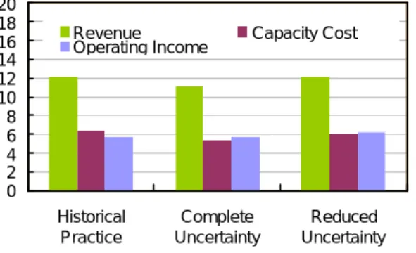
Figure 6. Trajectories of capacity increment The revenue, operating income and capacity cost of the two trajectories are compared with those of the historical trajectory in Figure 7. Following the option-based approach, the capacity cost will be lower but the operational income will be higher by a ratio between 0.1% and 7.6%. 0 2 4 6 8 10 12 14 16 18 20 Historical Practice Complete Uncertainty Reduced Uncertainty Revenue Capacity Cost Operating Income
Figure 7. Income of capacity trajectories
四、結論與成果
In this project, the rationality of capacity trajectory of a major semiconductor manufacturing company is analyzed at the aggregate level of capacity. Our analysis has shown that the option-based approach could generate a capacity plan that requires less investment, but generates higher operating income in the long term.
REFERENCES
[1] Shabbir Ahmed, “Semiconductor Tool Planning via Multi-stage Stochastic
Programming,” Proc. of 2002 Int. Conference on Modeling and Analysis of Semiconductor Manufacturing, Tempe, Arizona, U.S.A., 153-157, Apr. 2002.
[2] Francisco Barahona, Stuart Bermon, Oktay Gunluk, and Sarah Hood, "Robust Capacity
Planning in Semiconductor Manufacturing," Research Report RC22196, IBM, 2001.
[3] Dario L. Benavides, et al, “As Good as It Gets: Optimal Fab Design and Deployment,” IEEE Transactions on Semiconductor Manufacturing, Vol. 12, No. 3, 281-287, 1999.
[4] Avanish K. Dixit and Robert S. Pindyck,
Investment under Uncertainty , Princeton
University Press, 1994.
[5] D. Gary Eppen, R. Kipp Martin, and Linus Schrage, “A Scenario Approach to Capacity Planning,” Operations Research, Vol.37, No. 4, 517-527, 1989.
[6] A. Robert Jarrow and Andrew Rudd, Option
Pricing, Irwin, USA, 1983. [7] Suleyman Karabuk; S. David Wu,
“Coordinating Strategic Capacity Planning in the Semiconductor Industry” Technical Report 99T-11, Dept of IMSE, Lehigh University, 2001.
[8] J. M. Swaminathan, "Tool Capacity Planning for Semiconductor Fabrication Facilities under Demand Uncertainty," European Journal of Operations Research, Vol. 120, 545-558, 2000.
[9] Ruey S. Tsay, Analysis of Financial Time
Series, New York, United States of America,
![Figure 2: Sample paths of the demand process To facilitate numerical computation, the binominal model of Jarrow and Rudd [6] is then used to approximate the continuous demand process (Figure 3)](https://thumb-ap.123doks.com/thumbv2/9libinfo/8852614.242860/4.894.105.413.534.683/figure-facilitate-numerical-computation-binominal-approximate-continuous-figure.webp)