應用在文件分類的領域空間權重機制

全文

(1)國立交通大學資訊科學系碩士論文. 應用在文件分類的領域空間權重機制 Domain-space Weighting Scheme for Document Classification. 研究生：鄭佩琪指導教授：曾憲雄. 博士. 中華民國九十三年六月.

(2) 應用在文件分類的領域空間權重機制 Domain-space Weighting Scheme for Document Classification. 研究生：鄭佩琪. Student：Pei-Chi Cheng. 指導教授：曾憲雄. Advisor：Shian-Shyong Tseng. 國立交通大學資訊科學研究所碩士論文 A Thesis Submitted to Institute of Computer and Information Science College of Electrical Engineering and Computer Science National Chiao Tung University in partial Fulfillment of the Requirements for the Degree of Master in Computer and Information Science June 2004 Hsinchu, Taiwan, Republic of China. 中華民國九十三年六月.

(3) 應用在文件分類的領域空間權重機制. 研究生：鄭佩琪國. 立. 指導教授：曾憲雄博士交. 通大學電機資資訊科學系. 訊. 學. 院. 摘要隨著電子式文件的發展與增多，自動化文件分類(automatic document classification)在為使用者發掘和管理資訊上越來越重要。許多典型的分類方法，例如：C4.5，SVM，naïve Bayesian 等，已被應用於發展文件分類器(classifier)。然而，這些方法大部份是批次處理(batch-based)的探勘技術，無法處理分類器在類別隨時間變化而增加的適應問題(category adaptation problem)。另外，關於文件表示的問題(document representation problem)，大部份的表示法是以詞語空間(term-space)表示文件，可能產生許多沒有代表性的維度，使得分類器的效率和有效性因而降低。. 本論文提出一個領域空間權重機制 (domain-space weighting scheme)，將文件以領域空間(domain-space)的表示法表示，並以漸進式 (incremental)的方法建立文件分類器，解決上述的類別適應問題和文件表示問題。此機制包含三個階段：訓練階段(Training Phase)、鑑別階段 (Discrimination Phase)和微調階段(Tuning Phase)。在訓練階段，此機制針對各個類別萃取出足以代表該類別的特徵，並依其對該類別的重要性給. I.

(4) 予權重值，再將結果儲存於特徵領域關聯權重表 (feature-domain association weighting table)中，該表是用於記錄特徵與所有相關領域的關聯程度的表格。接著進入鑑別階段，此機制調降在分類時鑑別力小的特徵的權重值，以減低其對分類的影響力。至此，根據特徵領域關聯權重表，分類器已建置完成。而微調階段是選擇性的，利用微調文件的資訊加強分類器的分類能力。在實驗時，我們使用標準的測試文件集 Reuters-21578 based on the “ModApte” split version 評估所建置的分類器。實驗結果顯示，在有足夠的訓練文件下，分類器更加有效；而藉由微調階段，分類器更為強化。. II.

(5) Domain-space Weighting Scheme for Document Classification. Student : Pei-Chi Cheng. Advisor : Dr. Shian-Shyong Tseng. Institute of Computer and Information Science National Chiao Tung University. Abstract As evolving and available of digital documents, automatic document classification (a.k.a. document categorization) has become more and more important for managing and discovering useful information for users. Many typical classification approaches, such as C4.5, SVM, Naïve Bayesian and so on, have been applied to develop a classifier. However, most of them are batch-based mining approaches, which cannot resolve the category adaptation problem; and referring to the document representation problem, the representations are usually in term-space, which may result in lots of less representative dimensions such that the efficiency and effectiveness are decreased.. In this thesis, we propose a domain-space weighting scheme to represent documents in domain-space and incrementally construct a classifier to resolve both document representation and category adaptation problems. The proposed scheme consists of three major phases: Training Phase, Discrimination Phase and Tuning Phase. In the Training Phase, the scheme first incrementally extracts and weights features from each individual category, and then integrates the results into the feature-domain association. III.

(6) weighting table which is used to maintain the association weight between each feature and all involved categories. Then in the Discrimination Phase, it diminishes feature weights with lower discriminating powers. A classifier can be therefore constructed according to the feature-domain association weighting table. Finally, the Tuning Phase is optional to strengthen the classifier by the feedback information of tuning documents. Experiments over the standard Reuters-21578 benchmark based on the “ModApte” split version are carried out and the experimental results show that with enough training documents the classifier constructed by our proposed scheme is rather effective and it is getting stronger by the Tuning Phase.. Keywords: text classification, document representation, dimension reduction, term weighting.. IV.

(7) 誌謝. 這篇論文的完成，最感謝的是指導教授曾憲雄博士耐心的指導和勉勵，以及在待人處世方面的啟發，在此致上最誠摯的敬意和感謝。. 感謝口試委員何正信教授、李允中教授和洪宗貝教授，在百忙之中審閱論文，並提供許多寶貴的意見，讓此篇論文更有價值和意義。. 感謝實驗室學長、同學及學弟妹的幫助與鼓勵。特別謝謝慶堯學長，在論文的研究過程中不斷提出多層面的思考及討論，使論文更加完整。感謝家瑜、于彰、建豪、培綺、王威、力豪、哲青及斯聰對我的協助、支持與鼓勵。. 感謝文服的好友們，依潔、孟君、博聲、逸璿、家銘、偉志、東樺、淯正、瀅弘、禕翔、智凱、明瑋、羅傑、俐瑀、柏成、致青，豐富我的生活。感謝我的室友，筱筠、嘉玲和桂如，傾聽我的的憂愁、分享我的快樂，讓忙碌的碩士生涯更有趣、更有回憶。. 感謝所有曾經關心我、照顧我的人。最後要感謝家人對我的栽培和鼓勵，家人的支持是我最大的動力。. V.

(8) Table of Content 摘要............................................................................................................................................. I Abstract .....................................................................................................................................III 誌謝............................................................................................................................................V Table of Content....................................................................................................................... VI List of Figures ......................................................................................................................... VII List of Tables..........................................................................................................................VIII List of Algorithms .................................................................................................................... IX Chapter 1: Introduction ...............................................................................................................1 Chapter 2: Related Work.............................................................................................................4 2.1 Document Representation.............................................................................................4 2.2 Classifier Construction..................................................................................................5 2.3 Classifier Evaluation.....................................................................................................8 Chapter 3: Domain-space Weighting Scheme for Document Classification ............................11 Chapter 4: Classifier Construction Based on Domain-space Document Representation .........14 4.1 Training Phase.............................................................................................................17 4.2 Discrimination Phase ..................................................................................................19 4.3 Tuning Phase...............................................................................................................21 Chapter 5: Document Labeling by the Constructed Classifier .................................................25 Chapter 6: Experiments.............................................................................................................27 6.1 Experimental Setting...................................................................................................27 6.2 Experimental Results Analysis ...................................................................................27 Chapter 7: Conclusions and Future Work .................................................................................36 Bibliography: ............................................................................................................................38. VI.

(9) List of Figures Figure 1: An Example of the Support Vector Machine Approach ....................................6 Figure 2: The Classifier Construction Algorithm ...........................................................15 Figure 3: The Processing Procedure of the Classifier Construction Algorithm..............16 Figure 4: The Training Algorithm...................................................................................18 Figure 5: The Discrimination Algorithm ........................................................................20 Figure 6: The Tuning Algorithm .....................................................................................23 Figure 7: The Document Labeling Algorithm ................................................................25 Figure 8: The Curve of Micro-averaging F1 Values along with Different Tuning Documents for Reuters-21578(10) .................................................................................32 Figure 9: The Curve of Micro-averaging F1 Values along with Different Tuning Documents and at φ =1, φ =15 and φ =25 for Reuters-21578(90) .................................33 Figure 10: The Curve of Micro-averaging F1 Results along with Different Tuning Documents at φ =1, φ =15 and φ =25 for Reuters-21578(115) ......................................33 Figure. 11: The Computation Time Spent by the Batch-based Classifier and the Incremental-based Classifier for Reuters-21578(10)......................................................35. VII.

(10) List of Tables Table 1: The Micro- and Macro-averaging Performance Scores of the Precision and Recall ................................................................................................................................9 Table 2: An Example of the Feature-domain Association Weighting Table ...................13 Table 3: The Statistic Information of Features in“DM”Category ...................................19 Table 4: The Feature Weights in “DM” Category ...........................................................19 Table 5: An Example of the Tuning Algorithm on the Constructed Classifier. ..............24 Table 6: Micro- and Macro-averaging F1 Shown in [7] .................................................29 Table 7: Micro- and Macro-averaging F1 Values Respectively at φ =1, φ =15 and φ =25 for Reuters-21578(10), Reuters-21578(90) and Reuters-21578(115).............................29 Table 8: Micro-and Macro-averaging F1 Values at Different δ for Reuters-21578(10)..30 Table 9: Micro-averaging F1 Values at Different δ and φ for Reuters-21578(90) ..........30 Table 10: Macro-averaging F1 Values at Different δ and φ for Reuters-21578(90) .......31 Table 11: Micro-averaging F1 Values at Different δ and φ for Reuters-21578(115) ......31 Table 12: Macro-averaging F1 values at different δ and φ for Reuters-21578(115).......31 Table 13: Numbers of the Remaining Categories at Different φ ....................................31 Table 14: Micro-averaging F1 Results with Different Tuning Documents on Reuters-21578(90) with Different φ ...............................................................................34 Table 15: Micro-averaging F1 Results with Different Tuning Documents on Reuters-21578(115) with Different φ..............................................................................34. VIII.

(11) List of Algorithms Classifier Construction Algorithm: .................................................................................15 Training Algorithm: ........................................................................................................18 Discrimination Algorithm: ..............................................................................................20 Tuning Algorithm:...........................................................................................................23 Document Labeling Algorithm: ......................................................................................25. IX.

(12) Chapter 1: Introduction As evolving and available of digital documents, automatic document classification (a.k.a. document categorization) has become more and more important for managing and discovering useful information for users. Automatic document classification is the activity of automatically constructing classifiers to assign the category label for an undefined document according to the suggestion of pre-defined training documents. In general, automatic document classification involves three major tasks [27]: document representation, classifier construction, and classifier evaluation. Document representation is to represent a document a machine-readable structure, classifier construction is to construct a classifier for the pre-defined training documents, and classifier evaluation is to evaluate the classification accuracy of a classifier in terms of different evaluation functions.. In document representation, most of previous studies often represent a document by a finite set of terms such as keywords and phrases. For example, a document can be represented as <w1, w2, w3, …, wt> where t is the number of keywords and wi represents an association weight between i-th keyword and the document. It is called term-space document representation in this thesis. Although this representation is simple, it may result in large size of a document vector such that high computation time is required. On the other hand, it may result in lots of less representative dimensions because of highly correlated and redundant keywords. Both the efficiency and effectiveness of a classifier are decreased [12][13].. As for classifier construction, most of previously proposed approaches such as C4.5 [25], SVM [9][15][16] and Naïve Bayesian [23] are batch-based mining 1.

(13) approaches which have to reconstruct the classifier when new documents or new categories are added [24]. Since they cannot utilize previously discovered information for later maintenance, considerable computation time to get the updated classifier is required. In real world, the content of datasets may evolve along with time, and a batch-based classifier construction approach is obviously impractical.. In this thesis, we propose a domain-space weighting scheme to represent documents in domain-space and construct a classifier incrementally to resolve the above-mentioned document representation and category adaptation problems. The proposed domain-space document representation is a novel dimension reduction approach to represent each document by a finite set of domains. For example, a document can be represented as <w1, w2, w3, …, wc>, where c is the number of involved domains and wi represents the association weight between this document and the i-th domain. Comparing to term-space document representation, the domain-space document representation is more compact and meaningful.. The proposed scheme utilizes three phases, namely Training Phase, Discrimination Phase and Tuning Phase, to construct a classifier and adapt it along with evolving data. In the Training Phase, the scheme incrementally extracts and weights features from each individual category (in this thesis, a category is treated as a domain) in the training documents, and integrates the resulting association weights into the feature-domain association weighting table which is used to maintain the association weights between each feature and all involved categories. In the Discrimination Phase, it diminishes the association weights of the features having lower discriminating powers in the feature-domain association weighting table. The association weight between a document and each category can be easily calculated by 2.

(14) summarizing related feature weights in the feature-domain association weighting table, and the classifier is thus constructed according to this table. Finally, in the Tuning Phase, the scheme utilizes the feedback information from the tuning documents (the other pre-defined documents) to reduce the number of false positives for the constructed classifier.. We experiment the constructed classifier over the standard benchmark Reuters-21578 text collection [21] based on the “ModApte” split version in terms of micro- and macro-averaging F1 evaluation functions. The experiments consist of four aspects: (1) the classification accuracy of our classifier comparing to the algorithms shown in [7]; (2) the influence of the training document threshold φ and the discrimination threshold δ on the classification accuracy; (3) the influence of the number of tuning documents on the classification accuracy; and (4) the time performance of our classifier comparing to a batch-based mining approach. The experiment results show that the classification accuracy of our classifier is getting better with enough training documents, and the classifier is getting stronger by the Tuning Phase.. The remainder of this thesis is organized as follows. The related work for the activity of automatic document classification is briefly reviewed in Chapter 2. The domain-space weighting scheme for document classification is introduced in Chapter 3. The classifier construction based on domain-space document representation is proposed in Chapter 4. The document labeling by the constructed classifier is described in Chapter 5. The experimental settings, results and analysis are illustrated in Chapter 6. Finally, conclusions and future work are summarized in Chapter 7.. 3.

(15) Chapter 2: Related Work In the following, the previously related studies of three major tasks: document representation, classifier construction and classifier evaluation in automatic document classification will be briefly described.. 2.1 Document Representation Document representation is to represent a document in a machine-readable structure such that the classifier can be constructed efficiently and effectively by classifier construction. The most common approach is the vector space model (VSM), which represents a document by a set of features. The VSM usually considers two factors: (1) how to extract representative features from a document, and (2) how to decide the weight of a feature for a document. The term-space document representation which utilizes a finite set of keywords or phrases occurred in the document as representative features and decide the weight of a feature by the standard tfidf weighting function is the most popular form of vector space model. However, the term-space document representation may result in large size of a document vector such that high storage space and computation time is required. It may also result in lots of less representative features because of highly correlated and redundant keywords. Both the efficiency and effectiveness of a classifier are decreased [12][13].. Recently, the technique of dimension reduction attempts to resolve this problem. Among them, the approaches by term evaluation functions such as chi-square [10][30][32],. information. gain. [10][15][30][32]. and. mutual. information. [9][10][30][32], select the terms, which contribute the classification most, from the 4.

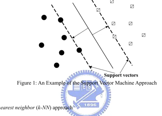
(16) original term set. Dimension reduction by term extraction functions, like term clustering technique [2][5][11][17][18], latent semantic indexing (LSI) [3][8], and ontology guided approaches [29], obtains new representative features by combinations or transformations of the old terms.. 2.2 Classifier Construction Rocchio approach Given a set of training documents, the Rocchio approach [22][26] attempts to learn a set of features used to represent each individual category from both positive training documents (if the training document is a member of this category) and negative training documents (if the training document is not a member of this category). Each category vector is calculated according to the formula: w j = αw1, j + β. ∑. i∈C. nC. d i, j. −γ. ∑. i∉C. d i, j. n − nC. ,. where wj denotes the j-th entry in the category vector, n denotes the number of training documents, C denotes the set of positive training documents, nC denotes the number of positive training documents, and the parameters α, β and γ denote the relative importance of the original entry of this category vector, the positive documents and the negative documents, respectively. Then an undefined document x is assigned to the category w when the inner product result of w and x is more than a user-specified threshold.. Support Vector Machine (SVM) approach Given a set of training documents, the support vector machine approach (SVM) [9][15][16] finds the best decision hyper-plane that separates two categories with the 5.

(17) maximum margin of each category. Take 2-dimensional case as an example, in Figure 1, the decision hyper-plane is determined by only a few training documents, called the support vectors, to find the maximum distance between different categories. Then an undefined document is assigned to the category which it is most close to.. Support vectors. Figure 1: An Example of the Support Vector Machine Approach. K-nearest neighbor (k-NN) approach The K-nearest neighbor (k-NN) [14][35] is the simplest approach and easy to be implemented, since it just treats each training document as a case and stores it in the case base. This is rather different from most of classifier construction approaches which need to construct a model in advance. When classifying an undefined document d, the k-NN first finds k nearest neighbors of d from the retained cases in the case base and calculates the similarity scores between this document and categories of the k neighbors by the following formula:. score ( d , Ci ) =. ∑ sim(d , d. d j ∈kNN ( d ), d j ∈C i. j. ),. where sim(d, dj) is a similarity function which can be measured by the inner product of their corresponding document vectors. Then an undefined document is assigned to the most similar category according to the summarized similarity score. 6.

(18) Naïve Bayesian approach Given a set of training documents, the naïve Bayesian approach [20][23] attempts to compute the probability which an undefined document belongs to each individual category, and assigns it to the category with the highest probability. The probability P(ck|di) between an undefined document di and category ck is computed by the Bayes rule as follows: P (c k | d i ) =. P (c k ) P ( d i | c k ) . P(d i ). Then di is assigned to the category with the highest probability.. In above formula, P(di|ck) is hard to compute in reality. By the assumption that when conditioned on a particular category ck, a particular feature of di is conditionally independent of any other feature, P(di|ck) can be estimated as m. P (d i | c k ) = ∏ P(d ij | c k ), j =1. where dij is the j-th feature of di. Unfortunately the conditional independent assumption is seldom true in real world; otherwise the naïve Bayes approach is amazingly effective.. Decision tree approach The decision tree approach [4][25] constructs a decision tree by recursively splitting the training documents in terms of a user-specified criterion until all or most of the documents in the same leaf nodes belong to the same category labels. Then based on the constructed decision tree, an undefined document is assigned to the category label of the leaf node which the document is classified to.. 7.

(19) Neural network approach The neural network approach [6][19] constructs a network of units from a set of training documents, where the input units represent the features of the training documents and the output units represent the category labels. Then an undefined document is loaded into the input units according to its features and propagated forward through the constructed network of units until an output unit is reached. Therefore the undefined document is assigned to the category label of the reached output unit.. 2.3 Classifier Evaluation As a classifier is constructed, to evaluate its classification accuracy, the capability of making correct classification decisions, is an important subsequent task. Precision (π) and Recall (ρ) used in the field of information retrieval and adopted in document classification are the two well-known evaluation functions. However, calculating only the precision or the recall for a classifier sometimes may be misleading and insufficient. The evaluation function Fβ of considering them simultaneously is usually adopted recently. The Fβ is defined as follows:. Fβ =. ( β 2 + 1) * π * ρ , β 2π + ρ. where, the parameter β which ranging from 0 to ∞ denotes the importance of precision (π) and the importance of recall (ρ) for Fβ. As β = 0, Fβ is identical to π. By contrast, as β = ∞, Fβ is identical to ρ. Setting β = 1, which stands for equal importance of π and ρ for Fβ, is the most used. The formula of F1 is listed as below:. 8.

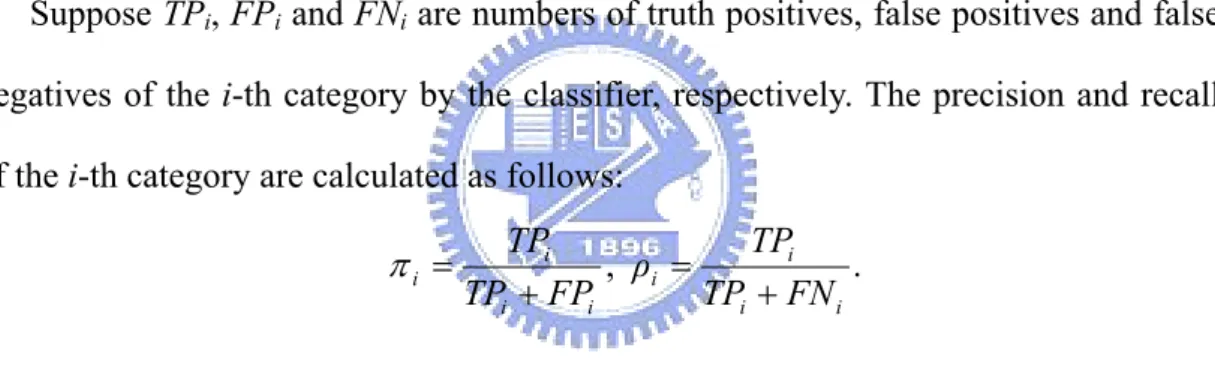
(20) F1 =. 2 *π * ρ . π +ρ. On the other hand, the evaluation functions are usually combined with micro-averaging or macro-averaging which evaluate the classification accuracy average across multiple categories. Micro-averaging performance score gives equal weight to each document classification decision and is therefore considered a per-document average, while macro-averaging performance score gives equal weight to each category without considering its frequency, i.e. a per-category average [33][34].. Suppose TPi, FPi and FNi are numbers of truth positives, false positives and false negatives of the i-th category by the classifier, respectively. The precision and recall of the i-th category are calculated as follows:. πi =. TPi TPi , ρi = . TPi + FPi TPi + FN i. Such that the micro- and macro-averaging performance scores of the precision and recall across c categories are calculated as Table 1:. Table 1: The Micro- and Macro-averaging Performance Scores of the Precision and Recall Precision Micro-averaging. ∑. µ. π =. ∑. i =1. c. i =1. Macro-averaging. πM =. c. ∑. TPi. (TPi + FPi ). c i =1. TPi TPi + FPi |c|. 9. Recall. ∑. µ. ρ =. ∑. c. i =1. ρM =. ∑. c i =1. TPi. (TPi + FN i ). c i =1. TPi TPi + FN i |c|.

(21) And the micro- and macro-averaging performance scores of F1 evaluation function are calculated as follows:. 2 *π µ * ρ µ , π µ + ρµ. Micro-averaging F1: F1µ =. Micro-averaging F1: F1M =. 10. ∑. c. i =1. (. 2 *π i * ρi ) π i + ρi . |c|.

(22) Chapter 3: Domain-space Weighting Scheme for Document Classification In term-space document representation, each document is represented by a finite set of terms, and each entry of a document vector represents the association weight between the term and this document. It may cause lots of less representative and redundant dimensions. As mentioned above, the technique of dimension reduction can be applied to resolving the problem. For example, dimension reduction by term selection approaches, such as [10][30][32] utilize complicated functions to select the best terms, which contributes the classification most, from the original term set, may be high computational requirement. And dimension reduction by term extraction approaches, such as [17] utilizes term clustering technique to group highly correlative terms together and replace them by the group center to reduce the redundant dimensions, and [29] utilizes a given concept ontology to map extracted terms into more meaningful concepts, may be problematic since they involve in uncertain determinant parameters when utilizing the clustering technique, or they need prior knowledge of concept ontology which is rare and seldom.. In this thesis, we propose a novel dimension reduction approach, called domain-space document representation, to represent each document by a finite set of domains. In the domain-space document representation, each category involved in the training documents is treated as a meaningful domain. A document can be represented as <w1, w2, w3, …, wc>, where c is the number of involved categories and wi represents the association weight between this document and the i-th category. Since the number of dimensions in domain-space is much less than that in term-space and irrelevant and redundant dimensions can be effectively reduced, the domain-space 11.

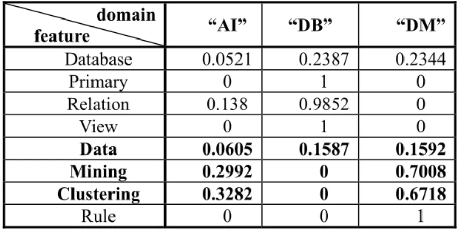
(23) document representation is more compact and representative than the term-space document representation. For each entry of the document vector, the larger association weight is, the more relative will be. Thus, according to the document vector, the entry with the maximum association weight is chosen to assign a category label for an undefined document.. In order to determine the association weight for each entry in the domain-space document representation, a feature-domain association weighting table is proposed to maintain the association weights between each feature and all involved categories. Since a document is made up of a set of keywords and a keyword can be treated as a representative feature, a document vector can be calculated by summarizing all its feature vectors in the feature-domain association weighting table. A document classifier can be thus constructed according to this table.. Example 1: Assume Table 2 is a feature-domain association weighting table in which there are three categories and eight keywords involved. For an undefined document d with three keywords, ‘Data’, ‘Mining’, and ‘Clustering’, its document vector can be calculated as < (0.0605+0.2992+0.3282)/3, (0.1587+0+0)/3 , (0.1592+0.7008+ 0.6718)/3 ) = < 0.2293, 0.0529, 0.5106 >. The d is thus assigned to the “DM” Category.. 12.

(24) Table 2: An Example of the Feature-domain Association Weighting Table domain feature Database Primary Relation View Data Mining Clustering Rule. “AI” 0.0521 0 0.138 0 0.0605 0.2992 0.3282 0. “DB” 0.2387 1 0.9852 1 0.1587 0 0 0. “DM” 0.2344 0 0 0 0.1592 0.7008 0.6718 1 ▀. The detail of constructing a feature-domain association weighting table will be described in the classifier construction algorithm in the next chapter.. 13.

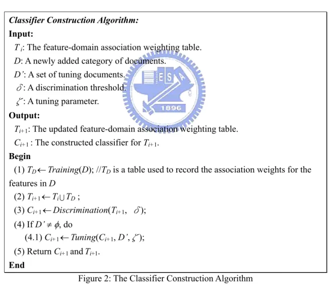
(25) Chapter 4: Classifier Construction Based on Domain-space Document Representation The proposed domain-space weighting scheme utilizes three phases, namely Training Phase, Discrimination Phase and Tuning Phase, to construct a classifier. In the Training Phase, the scheme incrementally extracts and weights features from each individual category in the training documents, and then integrates the results into the feature-domain association weighting table which is used to maintain the association weights between each feature and all involved categories. After that, in the Discrimination Phase, it diminishes the association weights for the features in the feature-domain association weighting table which have lower discriminating powers. The association weight between a document and each category can be easily calculated by summarizing related feature weights in the feature-domain association weighting table, and the classifier is thus constructed. Finally, in the Tuning Phase, the scheme utilizes the feedback information from the tuning documents (the other pre-defined documents) to reduce the number of false positives for the constructed classifier.. The proposed classifier construction algorithm is shown in Figure 2. It therefore contains three subroutines corresponding to the Training Phase, Discrimination Phase and Tuning Phase, respectively. Assume Ti is denoted as the feature-domain association weighting table in the i-th run. For a newly added category of documents D, the classifier construction algorithm first applies the training algorithm to extract and weight the features from this category D (Step 1) and then integrate the results into Ti (Step 2). Assume Ti+1 is denoted as the updated feature-domain association weighting table. Next it applies the discrimination algorithm to diminish the 14.

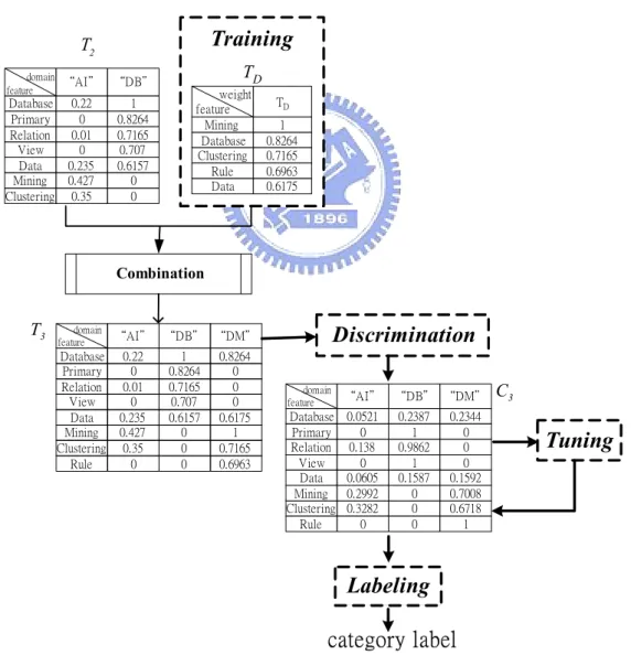
(26) association weights in Ti+1 for the features whose discriminating powers are less than the user-specified discrimination threshold δ. A classifier Ci+1 can be therefore constructed according to Ti+1 (Step 3). The tuning algorithm is optional, which depends on whether there exist tuning documents (Step 4). It can be used to strengthen the constructed classifier Ci+1 by a set of tuning documents D’ (Step 4.1), where the user-specified tuning parameter ζ is the tuning adjustment to increase or decrease the association weight in Ci+1 with ζ percent of feature weights in a tuning document.. Classifier Construction Algorithm: Input: T i: The feature-domain association weighting table. D: A newly added category of documents. D’: A set of tuning documents. δ: A discrimination threshold. ζ: A tuning parameter. Output: Ti+1: The updated feature-domain association weighting table. Ci+1 : The constructed classifier for Ti+1. Begin (1) TD ← Training(D); //TD is a table used to record the association weights for the features in D (2) Ti+1 ← Ti U TD ; (3) Ci+1 ← Discrimination(Ti+1, δ); (4) If D’ ≠ φ, do (4.1) Ci+1 ← Tuning(Ci+1, D’,ζ); (5) Return Ci+1 and Ti+1. End Figure 2: The Classifier Construction Algorithm. Example 2: Figure 3 illustrates the processing procedure of the classifier construction algorithm when a new category called “DM” is added. Assume T2 is the. 15.

(27) feature-domain association weighting table which has been constructed with the “OS” Category and the “DB” Category. When the “DM” Category is added, the training algorithm extracts and weights features from the “DM” Category. The results are stored in a table TD. After combining T2 and TD, the feature-domain association weighting table is updated as T3. The discrimination algorithm then diminishes the association weights in T3 for the features which have lower discriminating powers. The classifier C3 is thus constructed. The tuning algorithm can utilize the other given tuning documents to strengthen the classifier. The obtained classifier C3 can be used to classify an undefined document.. Training. T2 domain feature. Database Primary Relation View Data Mining Clustering. TD. “AI＂ “DB＂ 0.22 0 0.01 0 0.235 0.427 0.35. 1 0.8264 0.7165 0.707 0.6157 0 0. weight feature Mining Database Clustering Rule Data. TD 1 0.8264 0.7165 0.6963 0.6175. Combination. T3. domain feature. Database Primary Relation View Data Mining Clustering Rule. Discrimination. “AI＂ “DB＂ “DM＂ 0.22 0 0.01 0 0.235 0.427 0.35 0. 1 0.8264 0.7165 0.707 0.6157 0 0 0. 0.8264 0 0 0 0.6175 1 0.7165 0.6963. domain feature. Database Primary Relation View Data Mining Clustering Rule. “AI＂ “DB＂ “DM＂ 0.0521 0 0.138 0 0.0605 0.2992 0.3282 0. 0.2387 1 0.9862 1 0.1587 0 0 0. 0.2344 0 0 0 0.1592 0.7008 0.6718 1. C3. Tuning. Labeling category label Figure 3: The Processing Procedure of the Classifier Construction Algorithm ▀ 16.

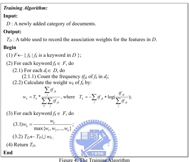
(28) 4.1 Training Phase. The purpose of the Training Phase in the domain-space weighting scheme is to extract representative features from a given category. In this thesis, the features are the keywords whose frequencies are more than one in at least one document in the given category, and they are extracted by a pre-processing procedure. The pre-processing procedure includes removing stop words [31], punctuation and digits, converting all letters into lowercase, and stemming by Porter’s stemmer. Since the training documents are belonging to the same category, a feature is more representative for a category if it appears in more documents and has higher frequencies in each document. The following formula is therefore designed to calculate the association weight wk of the feature fk for a given category, where tfjk denotes the frequency of feature fk in the document dj.. wk = Tk *. ∑ tf j. jk. ∑∑ tf jk k. , where Tk = −∑ tf jk ∗ log( j. j. tf jk. ∑ tf jk. ). (1). j. The proposed training algorithm is shown in Figure 4. When a newly category D is added, the training algorithm extracts all features from D (Step 1), and then calculates the association weight between each feature and D by considering the frequency and coverage of each feature against the documents in D by Formula 1 (Step 2.2). After all association weights of features have been obtained and calculated, the training algorithm normalizes them in range [0, 1] (Step 3.1), and adds them into the table TD which is used to record the association weights for the features in D (Step 3.2). Consequently, the training algorithm returns the association weighting table TD and terminates this algorithm (Step 4). 17.

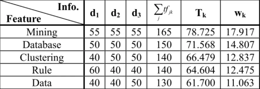
(29) Training Algorithm: Input: D : A newly added category of documents. Output: TD : A table used to record the association weights for the features in D. Begin (1) F ← { fk | fk is a keyword in D }; (2) For each keyword fk ∈ F, do (2.1) For each dj ∈ D, do (2.1.1) Count the frequency tfjk of fk in dj; (2.2) Calculate the weight wk of fk by: w k = Tk *. ∑ tf. jk. j. ∑ ∑ tf k. jk. , where Tk = −∑ tf jk ∗ log( j. tf jk. ∑ tf. ); jk. j. j. (3) For each keyword fk ∈ F, do wk (3.1) wk = ; max{w1 , w2 ,..., wk } (3.2) TD ← TD U wk ; (4) Return TD. End Figure 4: The Training Algorithm. Example 3: Assume there are five features, ‘Mining’, ‘Database’, ‘Clustering’, ‘Rule’ and ‘Data’, are extracted from the three documents d1, d2, d3 of the given “DM” Category. Table 3 shows the statistic information for these five features in the “DM” Category. According to Formula 1, the association weights between these five features and the “DM” Category are shown in Table 4. Among them, the feature weight of ‘Mining’ is calculated as follows:. w k = Tk *. ∑ tf. jk. j. ∑∑ tf k. = 78.725 * jk. 165 = 17.917, where ∑ tf jk = 165, ∑∑ tf jk = 725 and 725 j k j. j. 18.

(30) Tk = −∑ tf jk ∗ log( j. tf jk. ∑ tf. ) = (−55 log jk. 55 55 55 ) = 78.725 ) + (−55 log ) + (−55 log 165 165 165. j. After being normalized, the feature weight of ‘Mining’ is set at 1 as shown in Table 4.. Table 3: The Statistic Information of Features in“DM＂Category Info. Feature Mining Database Clustering Rule Data. d1. d2. d3. ∑tf. 55 50 40 60 40. 55 50 50 40 40. 55 50 50 40 50. 165 150 140 140 130. jk. j. Tk. wk. 78.725 71.568 66.479 64.604 61.700. 17.917 14.807 12.837 12.475 11.063. Table 4: The Feature Weights in “DM” Category TD. Feature Mining Database Clustering Rule Data. TD 1 0.8264 0.7165 0.6963 0.6175 ▀. 4.2 Discrimination Phase. The purpose of the Discrimination Phase in the domain-space weighting scheme is to diminish the association weights for the features in the feature-domain association weighting table which have lower discriminating powers. Specifically speaking, if a feature is not helpful for a classifier to decide the category label of a document, the classifier should diminish its importance for categories. The discriminating power of a feature can be evaluated by calculating the gini index value of its feature vector in the feature-domain association weighting table. Assume a feature vector fvk of a feature fk in the feature-domain association weighting table is. 19.

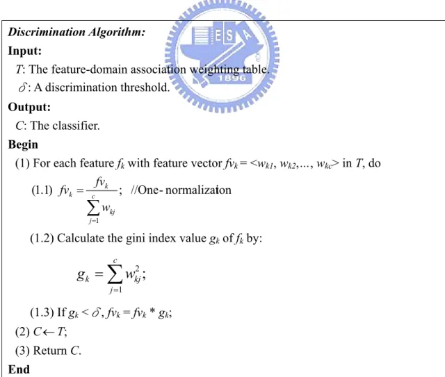
(31) represented as <wk1, wk2,…, wkc>, where wkj denotes the association weight between the feature fk and the j-th category. The gini index value gk of the feature fk can be calculated by the following formula:. gk =. c. ∑. j =1. w kj2 , where w kj =. w kj c. ∑. j =1. (2). w kj. The lowest gini index value appears when wk1 = wk2 = … = wkc = 1/c, whereas the highest gini index value appears when only one wkj = 1 and the rest ones are 0. This idea is conceptually similar to the idf term of the tfidf function. A feature has higher discriminating power if it is contained in fewer categories.. Discrimination Algorithm: Input: T: The feature-domain association weighting table. δ: A discrimination threshold. Output: C: The classifier. Begin (1) For each feature fk with feature vector fvk = <wk1, wk2,…, wkc> in T, do fv (1.1) fvk = c k ; //One - normalization ∑ wkj j =1. (1.2) Calculate the gini index value gk of fk by: c. g k = ∑ wkj2 ; j =1. (1.3) If gk <δ, fvk = fvk * gk; (2) C ← T; (3) Return C. End Figure 5: The Discrimination Algorithm. 20.

(32) The proposed discrimination algorithm is shown in Figure 5. According to Formula 2, the discrimination algorithm first normalizes each feature vector in the feature-domain association weighting table T such that ||fvk||1 = 1 (Step 1.1), and then calculates its corresponding gini index value (Step 1.2). After that, if the gini index value of a feature is less than the user-specified discrimination threshold δ, i.e. the discriminating power of this feature does not satisfy the minimum requirement, the discrimination algorithm diminishes the feature weights in T by multiplying the feature vector with its gini index value (Step 1.3). A classifier C can be therefore constructed (Step 2), since the association weight between a document and each category can be easily calculated by summarizing its related feature vectors in T. Consequently, the training algorithm returns the classifier C and terminates this algorithm (Step 3).. Example 4: Assume the discrimination threshold δ is set at 0.5. As in Figure 3, the discrimination algorithm will adjust the feature-domain association weighting table T3 to produce the classifier C3. For example, the feature vector of ‘Data’, <0.235, 0.6157, 0.6175>, in T3 is adjusted to <0.0605, 0.1587, 0.1592> in C3 as follows. First, one-normalization of ‘Data’ is <0.235/1.4682, 0.6157/1.4682, 0.6175/1.4682 > = <0.16, 0.4194, 0.4206>, and the gini index value of ‘Data’ is 0.162+0.41942+0.42062 = 0.3784. Since 0.3784 < 0.5, the original feature vector is diminished as <0.16, 0.4194, 0.4206> * 0.3784 = <0.0605, 0.1587, 0.1592>. ▀. 4.3 Tuning Phase. The purpose of the Tuning Phase in the domain-space weighting scheme is to 21.

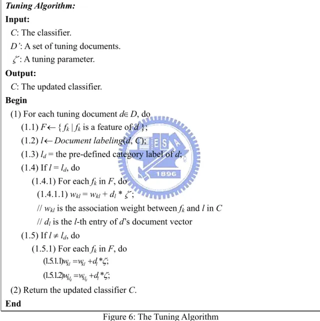
(33) utilize the feedback information from the tuning documents (the other pre-defined documents) to reduce the number of false positives for the constructed classifier. Specifically speaking, given a tuning document, the Tuning Phase first compares its pre-defined category label and the category label suggested by the constructed classifier. If consistent, it means that the classifier can correctly decide this tuning document by the corresponding feature vectors in the feature-domain association weighting table. Then the association weight between each corresponding feature and the category suggested by the classifier can be further emphasized, such that the classifier has strong association weights. Otherwise, it means that the classifier make incorrect decision by the feature-domain association weighting table. Then the association weight between each corresponding feature and the category suggested by the classifier should be diminished and the association weight between each corresponding feature and the pre-defined category of the tuning document should be emphasized, such that the classifier has appropriate association weights.. The proposed tuning algorithm is shown in Figure 6. For each given tuning document, the tuning algorithm first extracts its features (Step 1.1), and then obtains the category label suggested by the constructed classifier C (Step 1.2). The document labeling algorithm described in next subsection is used to carry out the suggestion procedure. If the category label suggested by C is consistent with the pre-defined category label of a tuning document, the tuning algorithm emphasizes the association weight between each corresponding feature and the suggested category with ζ percent of feature weight in the tuning document (Step 1.4.1.1), where ζ is the user-specified tuning parameter. Otherwise, the tuning algorithm diminishes the association weight between each corresponding feature and the suggested category with ζ percent of feature weight in the tuning document and emphasizes the association weight between 22.

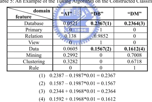
(34) each corresponding feature and the pre-defined category of a tuning document with ζ percent of feature weight in the tuning document (Step 1.5.1.1 and Step 1.5.1.2). Consequently, the tuning algorithm returns the updated classifier C and terminates this algorithm (Step 2).. Tuning Algorithm: Input: C: The classifier. D’: A set of tuning documents. ζ: A tuning parameter. Output: C: The updated classifier. Begin (1) For each tuning document d∈D, do (1.1) F ← { fk | fk is a feature of d }; (1.2) l ← Document labeling(d, C); (1.3) ld = the pre-defined category label of d; (1.4) If l = ld, do (1.4.1) For each fk in F, do (1.4.1.1) wkl = wkl + dl *ζ; // wkl is the association weight between fk and l in C // dl is the l-th entry of d’s document vector (1.5) If l ≠ ld, do (1.5.1) For each fk in F, do (1.5.1.1)wkl =wkl +dl *ζ; (1.5.1.2)wkld =wkld +dl *ζ;. (2) Return the updated classifier C. End Figure 6: The Tuning Algorithm. Example 5: Assume the tuning parameter ζ is set at 0.01 and a given tuning document d with two keywords, ‘Data’ and ‘Database’, is belonging to “DM” Category. According to the constructed classifier C3 in Figure 3, the document vector. 23.

(35) of d is thus <(0.0605+0.0521)/2, (0.1587+0.2387)/2, (0.1592+0.2344)/2> = <0.0563,0.1987,0.1968>, and then the classifier will assign the category label “DB” to d. Obviously, the constructed classifier C3 make incorrect decision by the obtained feature-domain association weighting table. Thus, the tuning algorithm will diminish the. association. weight. between. feature. ‘Data’ and. “DB”. Category. by. 0.1587-0.1987*0.01=0.1567 and emphasize the association weight between feature ‘Data’ and “DM” Category by 0.1592+0.1968*0.01=0.1612. On the other hand, the association weight between feature ‘Database’ and “DB” Category will be diminished by 0.2387-0.1987*0.01=0.2367 and the association weight between feature ‘Database’ and “DM” Category will be emphasized by 0.2344+0.1968*0.01=0.2364.. Table 5: An Example of the Tuning Algorithm on the Constructed Classifier. domain feature Database Primary Relation View Data Mining Clustering Rule (1) (2) (3) (4). “AI”. “DB”. 0.0521 0.2367(1) 0 1 0.138 0.9852 0 1 0.0605 0.1567(2) 0.2992 0 0.3282 0 0 0 0.2387 – 0.1987*0.01 = 0.2367 0.1587 – 0.1987*0.01 = 0.1567 0.2344 + 0.1968*0.01 = 0.2364 0.1592 + 0.1968*0.01 = 0.1612. “DM” 0.2364(3) 0 0 0 0.1612(4) 0.7008 0.6718 1. ▀. 24.

(36) Chapter 5: Document Labeling by the Constructed Classifier According to the classifier constructed by the domain-space weighting scheme, the association weight between a document and each category can be easily calculated by summarizing its feature vectors in the feature-domain association weighting table. For each entry of the document vector, the larger association weight is, the more relative will be. Thus, the classifier can choose the entry with the maximum association weight to assign a category label for an undefined document.. Document Labeling Algorithm: Input: d: An un-defined document. C: The classifier constructed by the classifier construction algorithm. Output: l: The category label for d. Begin (1) Vd ← 0; //Vd is the document vector of d and |Vd| equals the number of categories (2) For each features fk occurred in d, do (2.1) Extract the same feature vectors fvk with fk from C; (2.2) Vd = Vd + fvk; (3) Vd =. Vd ; // count(fk ) is the number of features in d count( f k ). (4) Return the category label l of the maximum association weight in Vd. End Figure 7: The Document Labeling Algorithm. The proposed document labeling algorithm is shown in Figure 7. Given an un-defined document d, the document labeling algorithm first uses the constructed classifier C to obtain the document vector Vd. This can be easily carried out by summarizing the feature vectors of features occurred in the document from 25.

(37) feature-domain association weighting table (Step 2 and Step 3). Then the document labeling algorithm can assign a category label for d according to the entry with the maximum association weight in Vd (Step 4).. Example 5: The same as Example 1, for a document d with three features ‘Clustering’, ‘Data’ and ‘Mining’, after looking up the feature-domain association weight table Table 2, d’s document vector is: <. 0.0605 + 0.2992 + 0.3282 0.1587 + 0 + 0 0.1592 + 0.7008 + 0.6718 > , , 3 3 3. = < 0.2293, 0.0529, 0.5106 >. So that the classifier will label d to the “DM” Category since the association weight between d and the “DM” Category is the largest. ▀. 26.

(38) Chapter 6: Experiments 6.1 Experimental Setting The experiments are implemented in Java on a personal computer with Pentium 1.7GHz processors and 512MB main memory, running Windows 2000 operation system. The experimental dataset is the standard benchmark Reuters-21578 text collection (“REUTERS-21578, Distribution 1.0”) [21] based on the “ModApte” split version. This dataset contains 118 categories of 12,902 documents, in which 9,603 documents are for training and 3,299 documents are for testing. According to the number of training and testing documents in a category, the following three selected groups of categories are used to evaluate the classification accuracy:. (I) The. 10. categories. with. the. largest. number. of. training. documents. (Reuters-21578(10)); (II) The 90 categories in which each contains at least one training document and one testing document (Reuters-21578(90)); (III) The 115 categories in which each contains at least one training document (Reuters-21578(115)).. 6.2 Experimental Results Analysis We experiment our classifier in terms of micro- and macro-averaging F1 evaluation functions with four aspects:. 27.

(39) (1) the classification accuracy of our classifier construction algorithm comparing to the algorithms shown in [7]; (2) the influence of the training document threshold φ and the discrimination threshold δ on the classification accuracy; (3) the influence of the number of tuning documents on the classification accuracy; (4) the time performance of our classifier construction algorithm comparing to a batch-based mining approach.. In [7], Debole and Sebastiani utilized six supervised term weighting functions, chi-square, information gain and gain ratio respectively globally or locally (i.e. χ2(g), IG(g), GR(g), χ2(l), IG(l), GR(l)), across three classifier construction algorithms, Rocchio, k-NN, and SVM, to compare the average classification accuracy respectively for Reuters-21578(10), Reuters-21578(90) and Reuters-21578(115). As shown in Table 6, we can find a classifier with GR(g) has the best classification accuracy. As for our classifier construction algorithm, if the discrimination threshold δ is set at 0.5 for Reuters-21578(10) and 0.04 for Reuters-21578(90) and Reuters-21578(115), and if the number of tuning documents is set at 0, Table 7 shows the classification accuracy of our classifier along with different training document threshold φ. The training document threshold φ is to determine whether a category in the training document is available. If the number of training documents in a category is less than the specified φ, the category is omitted in the training algorithm. For example, only 39 categories of Reuters-21578(90) satisfying φ = 25 are used in the training algorithm. From Tables 6 and 7, the classification accuracy of our classifier construction algorithm for Reuters-21578(10) is always better than that in [7], whereas the results of Reuters-21578(90) and Reuters-21578(115) are worse if φ is less than 15. We may conclude the classification accuracy of the classifier constructed by the domain-space 28.

(40) weighting scheme rather depends on the number of training documents and it will be getting better with enough training documents.. Table 6: Micro- and Macro-averaging F1 Shown in [7] Micro F1 Macro F1. Reuters-21578(10) Reuters-21578(90) Reuters-21578(115) Reuters-21578(10) Reuters-21578(90) Reuters-21578(115). χ2 (g) 0.852 0.795 0.793 0.725 0.542 0.596. IG(g) 0.843 0.750 0.747 0.707 0.377 0.458. GR(g) 0.857 0.803 0.800 0.739 0.589 0.629. χ2 (l) 0.810 0.758 0.756 0.674 0.527 0.581. IG(l) 0.816 0.767 0.765 0.684 0.559 0.608. GR(l) 0.816 0.767 0.765 0.684 0.559 0.608. Table 7: Micro- and Macro-averaging F1 Values Respectively at φ =1, φ =15 and φ =25 for Reuters-21578(10), Reuters-21578(90) and Reuters-21578(115) Micro F1 Macro F1. Reuters-21578(10) Reuters-21578(90) Reuters-21578(115) Reuters-21578(10) Reuters-21578(90) Reuters-21578(115). φ=1 0.903 0.751 0.737 0.824 0.490 0.616. φ =15 0.903 0.784 0.784 0.824 0.569 0.569. φ=25 0.903 0.815 0.815 0.824 0.660 0.660. The detail of the influence of the training document threshold φ and the discrimination threshold δ on the classification accuracy for Reuters-21578(10), Reuters-21578(90) and Reuters-21578(115) are respectively shown in Tables 8 to 12. As mentioned in the discrimination algorithm, the scale of δ is decided according to the number of categories. Thus, the scale range of δ in Table 8 is [1/10, 1], and the scale ranges of δ in Tables 9, 10 and in Tables 11, 12 are [1/90, 1] and [1/115, 1], respectively. Since each category in Reuters-21578(10) contains more than 50 training documents, the influence of the training document threshold is ignored in Table 8. From Tables 9 to 12, we can find the influence of δ is not obvious even for Reuters-21578(10) of categories with the largest number of training documents. The. 29.

(41) possible reason may be that the one-normalization of the discrimination algorithm has achieved the purpose of discrimination such that setting δ has less influence on the classification accuracy. Comparatively, setting φ has decisive influence on the classification accuracy. The larger number of training document is, the better classification accuracy will be.. Table 13 shows numbers of the remaining categories at different φ for Reuters-21578(10), Reuters-21578(90) and Reuters-21578(115). As φ is more than 15, Reuters-21578(90) and Reuters-21578(115) consider the same categories in the training algorithm.. Table 8: Micro-and Macro-averaging F1 Values at Different δ for Reuters-21578(10) δ 0.9 0.8 0.7 0.6 0.5 0.4 0.3 0.2 0.1. Micro-averaging F1 0.902511370 0.901324896 0.903302353 0.903302353 0.902906862 0.898951948 0.901324896 0.895788017 0.898160965. Macro-averaging F1 0.814721475 0.813716994 0.820149529 0.819969831 0.823657403 0.815825122 0.817534791 0.804622957 0.806951786. Table 9: Micro-averaging F1 Values at Different δ and φ for Reuters-21578(90) φ. δ 0.1 0.08 0.06 0.04 0.02 0.01. 1. 5. 15. 25. 35. 45. 0.74739 0.74827 0.75033 0.75063 0.74974 0.74974. 0.75360 0.75389 0.75478 0.75300 0.75271 0.75330. 0.78372 0.78403 0.78464 0.78433 0.78555 0.78555. 0.81300 0.81269 0.81458 0.81521 0.81553 0.81584. 0.82566 0.82631 0.82695 0.82824 0.8289 0.8289. 0.84547 0.84447 0.84681 0.84681 0.84681 0.84681. 30.

(42) Table 10: Macro-averaging F1 Values at Different δ and φ for Reuters-21578(90) φ. δ 0.1 0.08 0.06 0.04 0.02 0.01. 1. 5. 15. 25. 35. 45. 0.46830 0.48881 0.48748 0.48997 0.48467 0.48922. 0.52281 0.54619 0.53001 0.52214 0.51960 0.52176. 0.56963 0.57344 0.57152 0.56868 0.57205 0.57205. 0.66335 0.65812 0.66360 0.65998 0.66281 0.66312. 0.67258 0.67529 0.67395 0.67747 0.67783 0.67783. 0.71811 0.71390 0.71542 0.71738 0.71738 0.71738. Table 11: Micro-averaging F1 Values at Different δ and φ for Reuters-21578(115) φ. δ 0.1 0.08 0.06 0.04 0.02 0.01. 1. 5. 15. 25. 35. 45. 0.73593 0.73505 0.73711 0.73681 0.73652 0.73711. 0.74885 0.74915 0.7506 0.74944 0.74855 0.74915. 0.78372 0.78403 0.78464 0.78433 0.78555 0.78555. 0.81300 0.81269 0.81458 0.81521 0.81553 0.81553. 0.82566 0.82631 0.82695 0.82824 0.8289 0.8289. 0.71811 0.71390 0.71542 0.71738 0.71738 0.71738. Table 12: Macro-averaging F1 values at different δ and φ for Reuters-21578(115) φ. δ 0.1 0.08 0.06 0.04 0.02 0.01. 1. 5. 15. 25. 35. 45. 0.62378 0.60384 0.60474 0.61597 0.61526 0.61526. 0.53231 0.55127 0.53598 0.53130 0.53057 0.52903. 0.56963 0.57344 0.57152 0.56868 0.55990 0.57205. 0.66335 0.65812 0.66360 0.65998 0.66312 0.66281. 0.67258 0.67529 0.67395 0.67747 0.67783 0.67783. 0.71811 0.71390 0.71542 0.71738 0.71738 0.71738. Table 13: Numbers of the Remaining Categories at Different φ Reuters-21578(10) Reuters-21578(90) Reuters-21578(115). φ =1 10 90 115. φ =5 10 69 70. φ =15 10 51 51. 31. φ =25 10 39 39. φ =35 10 34 34. φ =45 10 27 27.

(43) After that, the influence of the number of tuning documents on the classification accuracy for Reuters-21578(10), Reuters-21578(90) and Reuters-21578(115) are respectively shown in Figures 8 to 10, where the tuning documents in our experiments are selected from the testing documents. The original testing documents are therefore divided into two parts for tuning and testing the constructed classifier, respectively. The tuning parameter ζ observed from the experimental results is set at 0.000005 to have a stably increasing trend. A too small ζ may cause that the tuning adjustment is so tiny that the tuning effects is insignificant, whereas a too large ζ may cause that the tuning adjustment is unstable and oscillatory such that the tuning effects become unpredictable. From Figures 8 to 10, it is easily seen that the classification accuracy of the constructed classifier is getting better along with increasing numbers of tuning documents and will be convergent as the tuning documents are more than 700.. Tuning on Reuters-21578(10). 0.95. F1 0.9. 0.85 0. 100. 200. 300. 400 500 600 700 Tuning documents. 800. 900 1000. Figure 8: The Curve of Micro-averaging F1 Values along with Different Tuning Documents for Reuters-21578(10). 32.

(44) Reuters-21578(90). micro F1. 0.85. 0.8 φ=1 φ=15. 0.75. φ=25. 0.7 0. 100. 200. 300. 400. 500. 600. 700. 800. 900. 1000. Tuning docs. Figure 9: The Curve of Micro-averaging F1 Values along with Different Tuning Documents and at φ =1, φ =15 and φ =25 for Reuters-21578(90). Reuters-21578(115). micro F1. 0.85. 0.8. φ=1 φ=15 φ=25. 0.75. 0.7 0. 100. 200. 300. 400. 500. 600. Tuning docs. 700. 800. 900. 1000. Figure 10: The Curve of Micro-averaging F1 Values along with Different Tuning Documents at φ =1, φ =15 and φ =25 for Reuters-21578(115). Tables 14 and 15 list the classification accuracy with different training document threshold on Reuters-21578(90) and Reuters-21578(115), respectively. We can further discover that by the tuning algorithm, the classifier with φ=15 have achieved the similar effect to the result of the classifier which is constructed with φ=25 but without the tuning algorithm.. 33.

(45) Table 14: Micro-averaging F1 Results with Different Tuning Documents on Reuters-21578(90) with Different φ Reuters-21578 (90) 0 φ=0 0.749449 φ=15 0.784027 φ=25 0.816159. Number of Tuning Documents 200 400 600 800 0.753614 0.757308 0.773390 0.788915 0.789430 0.793457 0.805179 0.818692 0.820750 0.826453 0.836256 0.845883. 1000 0.781840 0.815258 0.843235. Table 15: Micro-averaging F1 Results with Different Tuning Documents on Reuters-21578(115) with Different φ Reuters-21578 (90) 0 φ=0 0.736517 φ=15 0.784027 φ=25 0.816159. Number of Tuning Documents 200 400 600 800 0.740588 0.747276 0.765221 0.781122 0.789430 0.793457 0.805179 0.818692 0.820750 0.826453 0.836256 0.845883. 1000 0.773716 0.815258 0.843235. Finally, we want to evaluate the efficiency of our classifier construction algorithm compared with a batch-based classifier construction approach. Regardless of the tuning algorithm, the computation time of our classifier construction algorithm includes three major portions in the i-th run: (1) the time of extracting and weighting features from a given category, denoted as ti1; (2) the time of integrating the training results into the feature-domain association weighting table, denoted as ti2; and (3) the time of diminishing the association weights for the features in the feature-domain association weighting table which have lower discriminating powers, denoted as ti3. Since ti1 > ti2 >> ti3, the total computation time can be simplified as O(ti1+ti2) in i-th run. However, if our classifier construction algorithm mimics a batch-based approach which needs to re-process all previous categories so far to reconstruct the classifier in each run, the total computation time will be O( ∑ j =1 (t j1 + t j 2 ) ) in the i-th run. Figure i. 34.

(46) 11 shows the computation times spent by our classifier construction algorithm respectively in batch and in incremental for Reuters-21578(10) along with increasing number of involved categories. It is easily seen that, the computation time of the batch-based classifier is increasing along with the increasing number of involved categories whereas the computation time of the incremental-based classifier is almost the same along with increasing number of involved categories. Since the previous discovering information is all retained in the feature-domain association weighting table, the classification accuracy of the incremental-based classifier is the same as the batch-based classifier.. batch-based incremental-based. Efficiency on Reuters-21578(10). milliseconds. 800000 600000 400000 200000 0 T1. T2. T3. T4. T5 T6 category. T7. T8. T9. T10. Figure. 11: The Computation Time Spent by the Batch-based Classifier and the Incremental-based Classifier for Reuters-21578(10). 35.

(47) Chapter 7: Conclusions and Future Work This thesis proposes a domain-space weighting scheme to represent documents in domain-space and incrementally construct a classifier to resolve the document representation and categories adaptation problems. The scheme consists of three major phases: Training Phase, Discrimination Phase and Tuning Phase, and each of them has been successfully implemented according to corresponding algorithms. The training algorithm incrementally extracts and weights features from each individual category, and then integrates the results in a feature-domain association weighting table. The discrimination algorithm diminishes feature weights with lower discriminating powers. Consequently, the classifier is constructed according to the above two algorithms. Finally, the tuning algorithm strengthens the classifier by the feedback information of tuning documents to reduce the number of false positives for the constructed classifier. If the constructed classifier confronts with a set of newly inserting documents in which some belong to newly categories and the others belong to trained categories in the feature-domain association weighting table, the scheme will separate them first, and then apply the training algorithm in Section 4.1 to extract and weight features from documents of newly categories; as for the others of trained categories, the scheme will apply the tuning algorithm in Section 4.3 to extract newly information from them and integrate the result into the feature-domain association weighting table. Therefore, the scheme can deal with all newly inserting documents no matter what they belong to.. Experiments over the standard Reuters-21578 benchmark are carried out and the results show that the classifier with enough training documents is rather effective.. 36.

(48) And with the tuning algorithm, the classifier is getter stronger. In the future, we attempt to experiment over other document collections to validate our classifier construction algorithm. We will also try to employ other refined functions for the discrimination algorithm to enhance the performance. As for the tuning parameter in the tuning algorithm, we hope to construct a scheme to automatically learn an appropriate numeral for the tuning algorithm. We attempt to adapt our classifier construction algorithm on multi-label document classification in the future.. 37.

(49) Bibliography: [1] Antonie, M.L. and Zaiane, O.R. Text document categorization by term association. International conference on data mining, IEEE. 2002. [2] Baker, L. and McCallum, A. Distributional clustering of words for text classification. In SIGIR-98, 1998. [3] Berry, M.W., Dumais, S.T. and O’Brien, G.W. Using linear algebra for intelligent information retrieval. SIAM Review, 37:573-595, 1995. [4] Chickering D., Heckerman D., and Meek, C. A Bayesian approach for learning Bayesian networks with local structure. Proc. of 13th Conf. on Uncertainty in Artifical Intelligence, 1997. [5] Chu, W.W., Liu, Z. and Mao, Z. Textual document indexing and retrieval via knowledge sources and data mining. Communication of the institute of information and computing machinery, 2002. [6] Dagan, I., Karov, Y., and Roth, D. Mistake-driven learning in text categorization. Proc. of EMNLP-97, 2nd Conf. on Empirical Methods in Neural Language Processing, 1997. [7] Debole, F. and Sebastiani, F. Supervised term weighting for automated text categorization. ACM SAC, 2003. [8] Deerwester, S., Dumais, S.T., Furnas, G.W., Landauer, T.K., and Hashman, R. Indexing by latent semantic indexing. Journal of the American Society for Information Science, 41(6), 1990. [9] Dumais, S.T. and Chen, H. Hierarchical classification of web content. Proc. ACM-SIGIR Interformational Conference on Research and Development in Information Retrieval, pp. 256-263, Athens, 2000.. 38.

(50) [10] Dumais, S., Platt, J., Heckerman, D. and Sahami, M. Inductive learning algorithms and representations for text categorization. ACM CIKM, 1998. [11] Fuketa, M., Lee, S., Tsuji, T., Okada, M. and Aoe, J. A document classification method by using field association words. Jour. of information sciences, Elsevier Science. 2002. [12] Galavotti, L., Sebastiani, F. and Simi, M. Experiments on the use of feature selection and negative evidence in automated text categorization. Proc. of ECDL-00, 4th European Conf. on Research and Advanced Technology for Digital Libraries, 2000. [13] George H, J., Ron K. and Karl, P. Irrelevant features and the subset selection problem. In Proceedings of the 11 Machine Learning (1994) pp. 121-129. [14] Han, E.H. Text categorization using weight adjusted k-Nearest Neighbor classification. PhD thesis, University of Minnesota, October 1999. [15] Joachims, T. Text categorization with support vector machines: Linearing with many relevant features. Proc. of the 10th European Conference on Machine Learning, vol. 1938, pp. 137-142, Berlin, 1998, Springer. [16] Joachims, T. Making large-scale SVM learning practical. Advances in Kernel Methods-Support Vector Learning, Chapter 11, pp. 169-184. The MIT Press, 1999. [17] Karypic, G. and Han, E.H. Concept indexing: a fast dimensionality reduction algorithm with applications to document retrieval & categorization. CIKM, 2000. [18] Kim, Y.H. and Zhang, B.T. Document indexing using independent topic extraction. Proc. of the International Conference on Independent Component Analysis and Signal Separation (ICA). 2001.. 39.

(51) [19] Lam, S.L. and Lee, D.L. Feature reduction for neural network based text categorization. Proc. of DASAA-99, 6th IEEE International Conf. on Database Advanced Systems for Advanced Application, 1999. [20] Lweis, D.D. Representation and learning in information retrieval. PhD thesis, Department of Computer Science, University of Massachusetts, Amherst, US, 1992. [21] Lewis, D.D. Reuters-21578 text categorization test collection distribution 1.0. http://www.research.att.com/~lewis/reuters21578.html, 1999. [22] Lewis, D.D., Schapire, R.E., Callan, J.P. and Papka, R. Training algorithms for linear text classifiers. Proc. of ACM-SIGIR. 1996. [23] Lewis, D. Naïve (bayes) at forty: The independence assumption in information retrieval. In Tenth European Conference on Machine Learning. 1998. [24] Liu, R.L. and Lu, Y.L. Incremental context mining for adaptive document classification. ACM SIGKDD, 2002. [25] Quinlan, J.R. C4.5: Programs for machine learning. Moran Kaufmann, San Mateo, CA, 1993. [26] Rocchio, J.J. Relevance feedback in information retrieval. In The Smart Retrieval System-Experiments in Automatic Document Processing. P.313-323. Prentice-Hall, Englewood, Cliffs, New Jersey, 1971. [27] Sebastiani, F. Machine learning in automated text categorization. ACM Computing Surveys, 34(1): 1-47, 2002. [28] Shankar, S. and Karypis, G. Weight adjustment schemes for a centroid based classifier. TextMining Workshop, KDD, 2000. [29] Wang, B.B., McKay R.I., Abbass H.A., and Barlow M. A comparative study for domain ontology guided feature extraction. ACSC 2003.. 40.

(52) [30] Wibowo, W. and Williams, H.E. Simple and accurate feature selection for hierarchical categorization. Proc. of the symposium on document engineering, ACM. 2002. [31] Yang, Y. and Liu, X. A re-examination of text categorization. In Proc. of the 22nd Annual Int’l ACM SIGIR Conf. on Research and Development in Information Retrieval. Morgan Kaufmann, 1999. [32] Yang, Y. and Pedersen, J.O. A comparative study on feature selection in text categorization. Proc. of ICML-97, 14th International Conference on Machine Learning, pp. 412-420, 1997. [33] Yang Y. An evaluation of statistical approaches to MEDLINE indexing. In Proceedings of the American Medical Informatic Association (AMIA), pp. 358362, 1996. [34] Yang Y. An evaluation of statistical approaches to Text Categorization. Technical Report, CMU-CS-97-127, Computer Science Department, Carnegie Mellon University, 1997. [35] Zhou, S., Ling, T.W., Guan, J., Hu, J. and Zhou, A. Fast text classification: a training corpus pruning based approach. Proc. of the Eighth International Conf. on Database System for Advanced Applications, IEEE, 2003.. 41.

(53)