國立交通大學
應用化學系碩士班
碩士論文
利用電場調變紅外線吸收光譜研究溶劑效應對 1,2-二氯
乙烷構型平衡的影響
Infrared Electroabsorption Spectroscopic Study of the
Solvent Effect on the Conformational Equilibrium of
1,2-Dichloroethane
研究生:黃鎮遠
利用電場調變紅外線吸收光譜研究溶劑效應對
1,2-二氯乙烷構型平衡的影響
Infrared Electroabsorption Spectroscopic Study of the Solvent Effect on
the Conformational Equilibrium of 1,2-Dichloroethane
研究生:黃鎮遠 Student: Chen-Yuan Huang 指導教授:重藤真介 博士 Advisor: Dr. Shinsuke Shigeto
國 立 交 通 大 學 應用化學系碩士班
碩 士 論 文
A Thesis
Submitted to M. S. Program Department of Applied Chemistry
College of Science National Chiao Tung University in Partial Fulfillment of the Requirements
for the Degree of Master of Science in
Applied Chemistry
July 2012
Hsinchu, Taiwan, Republic of China
利用電場調變紅外線吸收光譜研究溶劑效應對
1,2-二氯乙烷構型平衡的影響
學生: 黃鎮遠 指導教授:重藤真介 博士
國立交通大學應用化學系碩士班
摘要
1,2-二氯乙烷是一個 C-C 單鍵內旋轉的簡單樣本模型。1,2-二氯乙烷存 在著兩種穩定的構型:間扭異構物以及對扭異構物。間扭異構物是具有極性 的,而對扭異構物是沒有極性的。因為這點不同,當 1,2-二氯乙烷與溶劑混 合的時候,溶劑的極性明顯地影響了兩個異構物之前的平衡關係。換句話說, 主導構型平衡的熱力參數,像是自由能變化(G)以及熵變化(S),會隨著 1,2-二氯乙烷在溶劑中的微觀環境發生明顯地反應這件事是被期待的。 在本研究中,我們利用電場調變紅外線吸收光譜研究 1,2-二氯乙烷以及 1,2-二氯乙烷與不同極性的有機溶劑混合(環己烷、四氯化碳、甲苯和氘代氯 仿等)對間扭異構物以及對扭異構物的構型平衡的影響。電場調變紅外線吸收 光譜是唯一可以實驗測定與構型平衡相關的自由能變化(G)的方法。自由能 變化(G)的數值由在環己烷中的3.12 (±0.11) kJ mol−1到純 1,2-二氯乙烷的1.34 (±0.09) kJ mol−1;此數據與一些極性表示刻度呈現負相關,像是介電常數、偶 極矩 ET(30) 等。利用已報告的焓變化的數值,我們可以估算熵變化(S)和兩 個異構物的自由體積的比例(Vg/Vt ),提供了其他方法難以取得的 1,2-二氯乙 烷對溶劑分子之間的分子間作用力的資訊。Infrared Electroabsorption Spectroscopic Study of the
Solvent Effect on the Conformational Equilibrium of
1,2-Dichloroethane
Student: Chen-Yuan Huang Advisor: Dr. Shinsuke Shigeto
M. S. Program, Department of Applied Chemistry
National Chiao Tung University
Abstract (in English)
1,2-Dichloroethane (DCE) is a simple model system for internal rotation around a C–C single bond. DCE occurs as two stable conformers: gauche and trans conformers. The gauche conformer is polar, whereas the trans conformer is nonpolar. Because of this difference, the equilibrium between the two conformers is profoundly affected by solvent polarity when DCE is mixed with solvent. In other words, the thermodynamic parameters dictating the conformational equilibrium, such as the free energy difference G and entropy difference S, are anticipated to sharply reflect microscopic environments around DCE in solvent.
In the present study, we use infrared (IR) electroabsorption spectroscopy to study the trans/gauche conformational equilibrium of pure DCE and DCE mixed with organic solvents having different polarity (cyclohexane, CCl4, toluene, and d-chloroform). IR
electroabsorption spectroscopy is the only method that can experimentally determine G associated with the conformational equilibrium. The G value changes from 3.12 (±0.11) kJ mol−1 in cyclohexane to 1.34 (±0.09) kJ mol−1 in pure DCE; it negatively correlates with polarity scales such as dielectric constant, dipole moment, and ET(30) value. Using
the reported values of the enthalpy difference H, we estimated the entropy difference S and free-volume ratio Vg/Vt between the two conformers, which provide otherwise
unobtainable information on intermolecular interactions between DCE and solvent molecules.
Acknowledgment
碩班的兩年研究學業生活順利的結束了,這段期間受到了很多
人在各方面的照顧與支持;首先,要感謝指導教授重藤真介老師,提供
一個良好的實驗環境及儀器,也教導我正確的研究技巧和態度;再來,
要感謝濱口宏夫老師提供參與研討會的學習機會;感謝傳耿學長在實驗
及生活上給予我很多幫助,並且一同為了論文奮鬥;感謝 Sudhakar Narra
學長常幫助我解決實驗上的困惑;感謝史習岡學長教會我我實驗操作及
分析;感謝偲偲學長、小阿芳學姊和辰文學長的照顧,讓剛加入這團隊
的我很快速的熟悉這間實驗室;感謝同屆的同學 apple 互相在實驗上的
勉勵完成研究;感謝學弟書瑋、君輔和恭慧幫忙處理實驗室裡的大小雜
事;感謝新進來的學弟妹帶給我許多的歡笑。
感謝許千樹教授實驗室的小毛學長在各方面給我很大的幫助,
讓我能夠完成我的碩士學位;感謝碩班的同學小偉、阿春、肉包、文哥
和丸子的陪伴讓我在碩班生活不會感到無聊;感謝我的好球咖勇龍、秋
祥、岱彥、辰恩以及學長學弟每周都陪我打球;感謝朋友給予我的鼓勵;
感謝于瑤總在我焦頭爛額的時候給我最大的支持與打氣;最後感謝我的
父母及家人給予我經濟上的支援,並且總是給予我支持與肯定,謝謝你
們每一位。
Tables of Contents
Page
Abstract (in Chinese) ... i
Abstract (in English) ... ii
Acknowledgment ... iii
Tables of Contents ... iv
List of Figures and Tables ... vi
Chapter I Introduction ... 1
Chapter II Theoretical background ... 6
II-1. Introduction ... 7
II-2. Absorbance change (A) spectra ... 7
II-3. Three distinct types of molecular response ... 7
II-3-1. Orientational polarization ... 8
II-3-2. Electronic polarization ... 13
II-3-3. Equilibrium shift ... 14
Chapter III Experimental ... 21
III-1. Introduction ... 22
III-2. Experimental setup ... 22
III-2-1. IR electroabsorption spectrometer ... 22
III-2-2. Sample cell ... 24
III-3. Sample preparation ... 27
III-4. Electroabsorption (A) and intensity difference (I) spectra ... 27
Chapter IV Infrared Electroabsorption Spectroscopic Study of the Solvent Effect on the Conformational Equilibrium of Liquid 1,2-Dichloroethane ... 34
IV-1. Introduction ... 35
IV-3. Methods and materials ... 40
IV-4. Results and discussion ... 41
IV-4-1. FT-IR spectra of pure DCE and binary mixtures of DCE ... 41
IV-4-2. IR electroabsorption spectra and band decomposition ... 42
IV-4-3. Solvent dependence of the thermodynamic parameters associated with the conformational equilibrium ... 44
IV-4-4. Electrostatic interaction parameter ... 46
Chapter V Conclusion ... 62
List of Figures and Tables
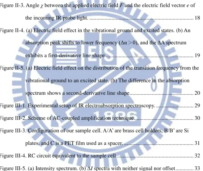
Page Figure ΙΙ-1. Coordinate system used in derivation of the orientational polarization signal.
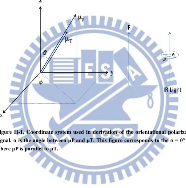
... 16 Figure II-2. Coordinate system used in derivation of the orientational polarization signal.
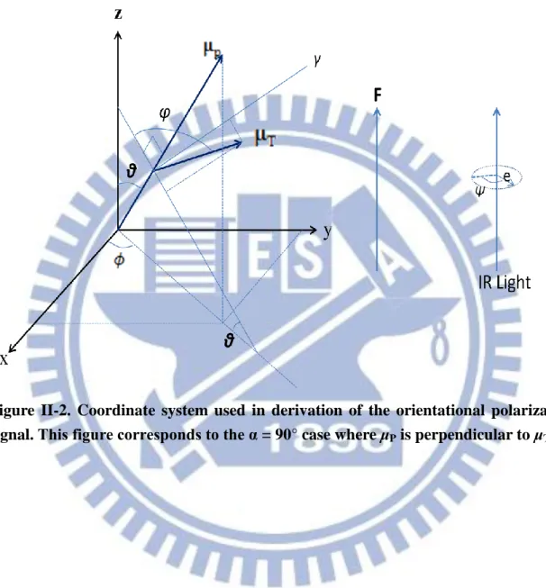
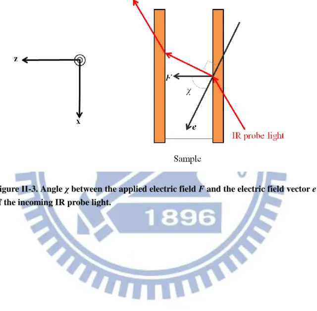
... 17 Figure ΙΙ-3. Angle χ between the applied electric field F and the electric field vector e of
the incoming IR probe light. ... 18 Figure ΙΙ-4. (a) Electric field effect in the vibrational ground and excited states. (b) An
absorption peak shifts to lower frequency (Δα>0), and the ΔA spectrum exhibits a first-derivative line shape ... 19 Figure ΙΙ-5. (a) Electric field effect on the distribution of the transition frequency from the
vibrational ground to an excited state. (b) The difference in the absorption spectrum shows a second-derivative line shape ... 20 Figure ΙIΙ-1. Experimental setup of IR electroabsorption spectroscopy. ... 29 Figure ΙIΙ-2. Scheme of AC-coupled amplification technique... 30 Figure ΙIΙ-3. Configuration of our sample cell. A/A’ are brass cell holders, B/B’ are Si
plates, and C is a PET film used as a spacer. ... 31 Figure ΙIΙ-4. RC circuit equivalent to the sample cell ... 32 Figure ΙIΙ-5. (a) Intensity spectrum. (b) I spectra with neither signal nor offset ... 33 Figure IV-1. (a) The trans/gauche conformational equilibrium of liquids
1,2-dichloroethane (DCE) and (b) Schematic diagram of the potential energy
of 1,2- ... 51
Figure IV-2. (a) FT-IR spectra of the pure DCE and the binary mixture of DCE in solvents (cyclohexane, CCl4, toluene, and chloroform) at mole fraction x=0.2.(b) The spectra normalized to the intensity of trans bands. ... 52
Figure IV-3. The spectra of pure DCE. ... 53
Figure IV-4. The spectra of DCE in d-chloroform at mole fraction x=0.2. ... 54
Figure IV-5. The spectra of DCE in toluene at mole fraction x=0.2. ... 55
Figure IV-6. The spectra of DCE in CCl4 at mole fraction x=0.2. ... 56
Figure IV-7. The spectra of DCE in cyclohexane at mole fraction x=0.2. ... 57
Figure IV-8. (a) Plot of K0 vs. dielectric constant (b) Plot of K0 vs. dipole moment (c) Plot of K0 vs. ET(30) ... 58
Figure IV-9. (a) Plot of G vs. dielectric constant (b) Plot ofG vs. dipole moment (c) Plot of G vs. ET(30) ... 59
Figure IV-10. (a) Plot of S vs. dielectric constant (b) Plot of S vs. dipole moment (c) Plot of S vs. ET(30). ... 60
Figure IV-11. (a) Plot of Vg/Vt vs. dielectric constant (b) Plot of Vg/Vt vs. dipole moment (c) Plot of Vg/Vt vs. ET(30). Free rotation limit ... 61
Table IV-1. Properties of solvents used in this study ... 48
Table IV-2: Assignments, conformations, symmetry species, peak positions, band widths of the three IR absorption bands observed for liquid 1,2-dichloroethane ... 48
Table IV-3: Fitting parameters used to reproduce theA spectra ... 49
Table IV-4: Solvent dependence of the experimental Gibbs free energy difference G, enthalpy difference H reported in the literature, and calculated entropy difference S between the gauche and trans conformers (gauche − trans) of 1,2-dichloroethane (DCE) in various solvents ... 49
Table IV-5: Solvent dependence of the translational entropy difference Strans in the free and frozen rotation limits and the free volumes, Vg and Vt, of the gauche and trans conformers. ... 50
Chapter I
Introduction
Chemistry relies largely on the interactions between charged particles. Because the electrostatic interactions between molecules and their surrounding occur invariably, they substantially influence the direction and rate of chemical reactions and hence play a central role in many branches of chemistry. Furthermore, the electrostatic interactions also profoundly affect fundamental molecular properties such as the permanent dipole moment, polarizability, and chemical bonding. It is therefore of great importance to elucidate these interactions via observing molecular responses to an externally applied electric field. Electroabsoption spectroscopy (also known as Stark spectroscopy), which directly probes the electrostatic interactions of molecules as responses to an external electric field, is a powerful technique for obtaining quantitative information on the electrostatic interactions in the condensed phase.
Stark spectroscopy provides unique information on molecular properties in diverse systems ranging from isolated gas-phase molecules to complex biological systems. The Stark effect [1, 2] has been extensively studied in the visible region [3-5]. A series of pioneering work was done by Liptay and co-workers [6]. They demonstrated experimental determination of electric properties of various aromatic molecules in solution [6]. In addition, they developed a theoretical basis of Stark spectroscopy [7], which is now widely used in this field. By working with frozen glasses at liquid N2 temperature, Boxer
and co-workers applied Stark spectroscopy to molecular systems such as donor-acceptor polyenes, transition metal complexes (metal-to-ligand and metal-to-metal mixed valence transitions), and nonphotosynthetic biological systems [4, 8]. They quantitatively discussed the amount of charge transfer based on two characteristic parameters obtained directly from experiment: the change in dipole moment, , and the change in polarizability, , between the ground and excited electronic states. Experimental values of and determined by Stark spectroscopy can also serve as a test for quantum
chemical calculations [9]. Ohta and co-workers [3, 10-12] examined the electric-field effects on absorption and fluorescence spectra of polymer films with specific dopant molecules. For instance, they obtained and of two different dopants (2-hydroxyquinoline or 6-hydroxyquinoline) embedded in a polymer film through temperature dependence experiments [12]. In another Stark study [11], they found that the photoirradiation of S3-PPV (sulfide-substituted PPV) in ambient air results in rapid degradation of the polymer film. These parameters and properties would be useful for developing and designing novel optical devices.
Because vibrational spectra are sensitive to molecular structures, one can expect that electroabsorption in the mid-infrared (mid-IR) region is an excellent tool for studying the Stark effect in relation to structural properties of molecules. To our knowledge, the first vibrational Stark measurement was carried out by Handler and Aspnes [13]. As early as in 1967, they applied IR electroabsoption spectroscopy to study the Stark effect on the O-H stretch mode of 2,6-diisopropyl phenol in CCl4 and obtained the parameters
associated with the dipole moment and the polarizability of the phenol derivative.
Close to 30 years later, in 1995 [14], Chattopadhyay and Boxer reported the use of vibrational Stark spectroscopy to study the electric-field effect on the C≡N stretch mode of anisonitrile in toluene at 77 K. They evaluated Δ and between the vibrational states involved. The Boxer group extended their vibrational Stark work to a series of compounds containing the CN group [15]. In 2002 [16], they applied the technique to free CO and CO bound to myoglobin (Mb). It is shown that the change in dipole moment for the CO bound to Mb is larger than that for the free CO because of d back-bonding. Extensive studies from the Boxer group have recently been reviewed [5].
These studies have all been performed in frozen glass at 77 K, where orientational motion of molecules is literally frozen or suppressed to a great extent. This experimental
condition enables one to interpret Stark spectra easily because the electronic response via
and are the only dominant contributions. However, those spectra lack in the information on the orientational response to an applied electric field, which is very useful for understanding molecular structures and association in liquid/solution.
Hiramatsu and Hamaguchi developed an electroabsorption spectrometer that is best suited for the IR region and room-temperature samples [17]. Using a dispersive IR spectrometer equipped with an alternating current (AC)-coupled amplifier, instead of using the FT-IR method, they were able to detect IR absorbance changes as small as 10−7. Hamaguchi and co-workers used their unique technique to investigate the trans/gauche conformational equilibrium of liquid 1,2-dichloroethane (DCE) [18], followed by the studies of self-association of N-methylacetamide in 1,4-dioxane [19], association forms of a liquid crystal (5CB) at different temperatures [20], and solvated forms of p-nitroaniline (PNA) in mixed solvents of acetonitrile and CCl4 [21]. In 2007, the whole system of the
IR electroabsorption spectrometer was transferred to NCTU and was reconstructed by our laboratory. Using the reconstructed setup, we studied the trans/gauche conformational equilibrium and associated thermodynamic parameters of liquid 1,2-dibromoethane [22] and solvated structures of N,N-dimethyl-p-nitroaniline in mixed solvents of acetonitrile and tetrachloroethylene [23]. We also attempted to observe the electric-field effects on the O–H stretch vibration of water dissolved in 1,4-dioxane[24].
In the present work, the author extends the previous study of the trans/gauche conformational equilibrium of pure liquid DCE to binary mixtures of DCE and organic solvents with various polarity. We observe IR electroabsorption spectra of DCE mixed with solvent and examine the solvent effect on the thermodynamic parameters associated with the conformational equilibrium, such as the equilibrium constant K0, Gibbs free
The rest of this thesis is organized as follows. In Chapter II, the theoretical background of IR electroabsorption spectroscopy is outlined. Major molecular responses to an externally applied electric field that contribute to IR absorbance changes are considered, and their mathematical expressions are derived. Chapter III provides a detailed description of our IR electroabsorption spectrometer and a home-made sample cell. Furthermore, we illustrate that an offset in the I spectrum possibly results in artifacts in the A spectrum, raising caution when analyzing the A spectrum. In Chapter IV, the author presents the results of his IR electroabsorption study of the solvent effect on the trans/gauche conformational equilibrium of DCE. Both FT-IR and IR electroabsorption spectra manifest the effect of solvent mixed with DCE as varying ratios of the CH2 wagging band of the trans form to that of the gauche form. We fit the observed
IR electroabsorption spectra to model functions and obtain the equilibrium constant K0 and associated thermodynamic parameters of DCE in the binary mixtures. Last, we discuss the physical meaning of the thermodynamic parameters so obtained and the correlation between the parameters and several polarity indices of solvents.
Chapter II
II-1. Introduction
In this chapter the theoretical background of IR electroabsorption spectroscopy is depicted in detail. To analyze an infrared electroabsorption (A) spectrum, three mechanisms of molecular responses to an externally applied electric field are to be considered: orientational polarization, electronic polarization, and equilibrium shift. Formulae are derived for absorbance changes arising from these responses. The equations derived here will be used in Chapter IV to analyze experimental data.
II-2. Absorbance change (A) spectra
When an electric field is externally applied to the sample, changes in absorption intensity are induced. The absorbance change (A) is calculated from the intensity change as on off on off 0 0 log log log 1 A A A I I I I I I (II -1)
Here is the intensity spectrum of the IR probe light. and I ( ) represent the
intensity spectra of the transmitted IR light through the sample with and without the applied electric field, respectively. I is the intensity difference spectrum, I = Ion –
Ioff.
II-3. Three distinct types of molecular response
In general, the absorbance change (A) can be attributed to three distinct types of molecular responses to an externally applied electric field: orientational polarization, electronic polarization, equilibrium shift [17, 18]. In what follows, we derive expressions for the A spectrum arising from each molecular response and see how those molecular
responses contribute to the overall A spectrum.
II-3-1. Orientational polarization
Consider a polar molecule that has a permanent dipole moment p. When we apply an external electric field to the sample, reorientation of the molecule takes place such that the dipole moment of the molecule aligns along the direction of the electric field. This response gives rise to orientational anisotropy. The induced polarization then contributes to changes in absorption spectrum.
(1) Normally incident nonpolarized light
To derive the expression for the orientational polarization signal, let us begin with the Beer–Lambert law:
2 2 2 T 0 0 0 1 1 sin d ( ) d d ( ) 2 2 A c c K f
e μ (II-2)where is the molar extinction coefficient, c the concentration of the sample (mol L−1), the path length (cm) of the sample, K a proportionality constant, the wavenumber (cm−1), and e a unit vector designating the direction of the electric field of the incident light. As shown in Figs. II-1 and II-2, we set molecule-fixed coordinates system such that the z-axis coincides with the direction of the applied electric field and the propagation direction of the IR light. The orientations of the permanent dipole moment μP and the
transition moment μT are specified by a set of angles ( , , ). In Eq. II-2, there are two
integrands to be evaluated explicitly; one is the spatial distribution function f , and the other is the square of the inner product of the transition moment and the unit vector,
2 T
(e μ ) .
the coordinate system shown in Figs. II-1 and II-2, we have p p sin cos sin sin , cos θ μ θ θ μ , 1 0 0 F F cos sin 0 e (II-3)
The probability is proportional to
T k E B
exp , with E being the dipolar interaction energy
T
P P P
sin cos 0
sin sin 0 cos cos 1 θ E μ θ F μ F θ μ F (II-4)
Thus the distribution function f becomes
p B cos
( ) C exp μ F C exp( cos )
f k T (II-5) with p B μ F k T . (II-6)
Here C is a normalization factor, T is the temperature, and is the Boltzmann constant, and F is the electric field strength. Note that the electric field F in Eq. II-6 is not the external field but local field which is exerted on individual molecules. The parameter reflects the magnitude of the electrostatic interaction and is a key quantity in evaluating μP.
The factor C is determined by the normalization condition
2 ( )s i n 1
0 0
f dd (II-7) In the presence of the electric field (F0), f()becomes from Eqs. II-5 and II-7on( ) 1 exp( cos ) 2 exp( ) exp( ) f (II-8)
Eq. II-8:
4 1 o f f f (II-9)The scalar product of and e can be calculated as follows. The electric field vector e, of the incident light lies in the xy-plane, and a projection of onto the xy-plane is related to (μ e . T )2 is expressed as
T T
cos cos cos sin sin sin sin cos sin cos sin cos cos sin cos sin sin sin sin cos sin cos sin cos cos
μ μ (II-10)
If is parallel to , i.e., α 0º as shown in Fig. II-1, Eq. II-10 reduces to
T T sin cos sin sin cos θ φ μ θ φ θ μ (II-11)
Using Eqs. II-3 and II-11, (e μ T)2 is obtained as
2 2 2 T T 1 ( ) sin 2μ θ e μ (II-12)
Here we have replaced , , and by their mean values in the range 0 2 (1/2, 1/2, and 1, respectively). In the absence of the external electric field, the absorbance for an α ° vibrational mode is calculated from Eqs. II-2, II-9, and II-12 as
2 2 off off T 0 0 2 2 3 T 0 0 2 T ( ) sin 1 1 sin d 4 2 1 3 A f d d d
e μ (II-13)Similarly, substitution of Eqs II-8 and II-12 into Eq. II-2 results in the absorbance for the α º mode when the electric field is turned on
2 2 on on T 0 0 2 T 2 3 ( ) sin 1 2 2 (e e ) (e e ) 2 (e e ) A f d d
e μ (II-14)By expanding the exponential functions and retaining terms up to second-order in , we have on 2 T2 6 2 A (II-15)
To confirm the validity of this approximation, suppose that 50 V is applied across liquid acetone 5 μm thick. The electric field strength is . For simplicity, we do not consider the local field correction. Using the dipole moment of acetone, μP = 2.8
D[17] (1 D = 3.33564 × 10⁻³⁰ C m), we obtain = 0.02, for which << 1 holds.
The absorbance change caused by the applied electric field is the difference between
(Eq. II-15) and (Eq. II-13). The absorbance change ratio is thus
6 2 2 o f f o f f on off A A A A A (II-16) Next we consider the α º case where is perpendicular to (Fig. II-2). Equation II-10 reduces to
T T
cos cos cos sin sin sin cos cos sin cos cos sin μ μ (II-17) 2 2 2 T T 1 ( ) (cos 1) 4μ θ μ e (II-18) Making use of Eqs. II-2, II-8, II-9, and II-18, we end up with the absorbance change ratio of the form 6) 2( 2 2 off A A (II-19)
Generalization of Eqs. II-16 and II-19 to an arbitrary angle is straightforward. The absorbance change for angle can be decomposed into its parallel ( ) and
perpendicular (α °) components as follows: 2 2 T T 0 90 cos sin A A A μ μ A A (II-20)
Substitution of Eqs. II-16 and II-19 into Eq. II-20 yields the following expression for the orientational polarization signal probed with the normal incidence
A A 1 3cos 6) 2( 2 2 2 (II-21)Again in the present study, so the first term in the denominator of the right-hand side of Eq. II-21 is safely neglected. Therefore we are left with
2 2 1 3 cos 12 A A (II-22)(2) p-Polarized light with tilted incidence
So far, we have considered the case where the electric field vector of the incident, nonpolarized light on the xy-plane is parallel to the sample cell. In other words, is equal to 90°, where is the angle between the applied electric field F and the electric field vector e of the incoming IR light (see Fig. II-3). When p-polarized light whose electric field vector e has only x-component is incident upon the sample with angle , the absorbance change ratio is shown to be given by [13]
2 p , 2 2 B 1 1 3 cos 1 3 cos 12 F A A k T , (II-23)It follows from Eq. II-23 that the orientational polarization signal disappears at
1 o
cos 1/ 3 54.7
. Furthermore, the orientational polarization A spectrum is
proportional to the absorption spectrum A, so that it appears as its zeroth derivative. An important application of Eq. II-23 is that the dipole moment μP can be experimentally
II-3-2. Electronic polarization
An absorbance change also arises from electronic polarization, which is associated with the change in electronic properties of molecule such as the dipole moment and the polarizability caused by an external electric field. This is well known as the Stark Effect. A general theory of the electronic polarization signal was established by Liptay and co-workers [6, 7]. In general, the electronic polarization spectrum is modeled by the following formula [25, 26]:
2
2
2 2 2 d d 15 d 30 d B A C A A F A A hc h c (II-24)where h is Planck’s constant and c is the speed of light. Although this equation may also include third and higher order derivatives, their contributions are expected to be negligible. Therefore, we consider here the derivatives up to second-order. For a randomly oriented, mobile molecule, the coefficients Aχ, Bχ, and Cχ are given by [25-27]
2 2 2 2 2 g g g g 2 B 2 g 2 2 2 gm g 2 2 B B 1 10 3 3 2 3cos 1 30 1 10 3 3 2 3cos 1 15 13cos 1 3cos 1 3cos 1
10 30 ij ii jj ij ji ij ij i ij j i ji j i jj i i ij j ij A A A A A A A m A m A m A m A k T k T k T
m m (II-25)
2 2 2 m g B 2 g g B 1 3 3 2 3cos 1 15 3 5 3cos 1 2 2 1 ˆ ˆ 3 3cos 1 i ij j i ji j i jj i i ij j ij B m A m A m A m A k T k T
m μ μ m μ m μ μ μ (II-26)
2 2 2 ˆ 5 3 3cos 1 C μ m μ μ (II-27)field dependence of the transition moment, m(F) = m + A • F. and denote the changes in dipole moment and polarizability tensor between the vibrational ground state (g) and an excited state (e), respectively, i.e., μ μeμg and α αe αg. mˆ is a unit vector in the direction of the transition dipole moment m (for consistency with the literature, we prefer to use m here for the transition moment instead of T). gm and m
are the components of the ground-state polarizability and the polarizability change along the direction of the transition moment, i.e., αgm m α mˆ g ˆ and m mˆ α mˆ . A bar
indicates the average value of the polarizability ( 1 1
g 3Tr g, 3Tr
).
The zeroth-derivative component represents the intensity change of the absorption spectrum. Note that the fourth term in Eq. II-25 is essentially identical to the orientational polarization contribution, which we already derived above. The first-derivative component depends on both and , and is responsible for the peak shift, as illustrated in Fig. II-4. The second-derivative component, which is characterized solely by , shows the band broadening of the absorption spectrum (see Fig. II-5)
II-3-3. Equilibrium shift
The shift of a chemical equilibrium caused by an external electric field can also contribute to the A signal. If the electrostatic interaction differs among molecular species coexisting in the equilibrium, the equilibrium would shift towards more stable species [18, 22]. To understand how absorbance changes result from the equilibrium shift, let us assume that two molecular species, C and D, coexist in equilibrium in the sample. Species C is nonpolar, whereas D is polar and interacts with an external electric field to a greater extent than species C does. When an electric field is applied to the sample, species D is stabilized via the electrostatic (dipolar) interaction. On the other hand, species C is little
increase and concomitantly that of species C decrease, so that the equilibrium between these two species shifts towards D. Thus, IR absorption of species D is expected to increase, whereas that of species C should decrease.
Since this equilibrium shift A signal is a change in absorption intensity, it has the same shape as the absorption spectrum and hence contributes to the zeroth derivative component as is the orientational polarization signal. The equilibrium shift signal does not depend on angle , so it is possible to differentiate between the orientational polarization and equilibrium shift contributions to the A spectrum by examining angle dependence of the A spectrum. More details of the equilibrium change signal will be given in Chapter IV, where we study the solvent effect on the trans/gauche conformational equilibrium of liquid 1,2-dichloroethane with IR electroabsorption spectroscopy.
Figure ΙΙ-1. Coordinate system used in derivation of the orientational polarization signal. α is the angle between μP and μT. This figure corresponds to the α = 0° case where μP is parallel to μT.
Figure II-2. Coordinate system used in derivation of the orientational polarization signal. This figure corresponds to the α = 90° case where μP is perpendicular to μT.
Figure ΙΙ-3. Angle χ between the applied electric field F and the electric field vector e of the incoming IR probe light.
(a)
(b)
Figure ΙΙ-4. (a) Electric field effect in the vibrational ground and excited states. (b) An absorption peak shifts to lower frequency (Δα>0), and the ΔA spectrum exhibits a first-derivative line shape (not to scale).
(a)
(b)
Figure ΙΙ-5. (a) Electric field effect on the distribution of the transition frequency from the vibrational ground to an excited state. (b) The difference in the absorption spectrum shows a second-derivative line shape (not to scale).
Chapter III
Experimental
III-1. Introduction
The IR electroabsoption spectroscopic system used in the present study was originally developed by Hiramatsu and Hamaguchi [17] and subsequently reconstructed at NCTU by our group[22, 23]. First, our experimental setup is described, followed by the details of our home-built sample cell. In order to develop a highly sensitive infrared electroabsorption system, we employ the alternating current (AC) coupled dispersive method. Owing to the combination of a dispersive spectrometer and an AC-coupled amplification technique, the detection limit of absorbance change is as low as A~10−7. Second, sample preparation for IR electroabsorption and FT-IR measurements are described. Last, possible effects of an offset in the I spectrum on the A spectrum are discussed. We show that the presence of an offset in the I spectrum most likely caused by the electronics may result in artifacts in the A spectrum.
III-2. Experimental setup
III-2-1. IR electroabsorption spectrometer
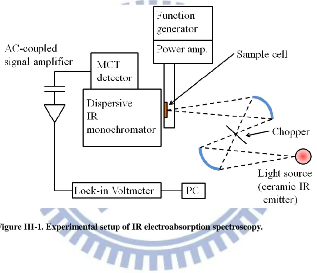
The experimental setup for IR electroabsorption spectroscopy is described in this section. A schematic of the experimental setup is shown in Fig. III-1. The system consists of a light source, a home-made sample cell, an optical chopper (Stanford Research System Inc. SR540), a dispersive IR monochromator, a photoconductive HgCdTe (MCT) detector (New England Research Center, MPP12-2-J3), an AC-coupled amplifier, and a lock-in amplifier (Stanford Research System Inc. SR844). The probe light source which we used to illuminate the sample was a ceramic mid-IR emitter (JASCO). As shown in Fig. III-1, the optical chopper and the sample cell were set at the co-focus of two ellipsoidal mirrors and at the other focus of the second ellipsoidal mirror, respectively. A chopper blade with 6 windows generated a modulation of 240 Hz to the probe light source. A function
generator (IWATSU, FG-330) produced an AC voltage (25 kHz sinusoidal wave) and after amplified by a power amplifier, the AC voltage was applied across the sample about 6 m thick. By combining the dispersive IR monochromator and the AC-coupled technique, the sensitivity to absorbance changes induced by electric field modulation reaches as high as , which is better than or at least comparable to that achieved by the latest FT-IR method.
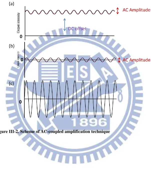
In this paragraph, the AC-coupled technique is briefly outlined. It is a powerful technique to detect a small AC component lying on top of a large DC offset. In the present case, the intensity of the transmitted IR probe light corresponds to the DC offset and an intensity change due to an external electric field corresponds to the AC component [Fig. III-2(a)]. The amplitude of the AC component is typically three or even higher orders of magnitude smaller than that of the DC offset. In order to detect such small AC amplitude, we used a low-noise preamplifier to remove the DC offset [Fig. III-2(b)] and amplified only the AC component. Then the output of the preamplifier was amplified once again [Fig. III-2(c)] by the main amplifier (Stanford Research System Inc. SR560, gain; ) and fed by the lock-in amplifier. In this way, only the intensity change due to the applied electric field can be detected with a wide dynamic range.
In IR electroabsorption measurements, three spectra are measured. (i) The intensity spectrum, I0, of the IR probe light without the sample. (ii) The intensity spectrum, I, of the
IR probe light with the sample. I0 and I are obtained using a digital sampling oscilloscope
(LeCroy, LC334-DSO) and the mechanical chopper operating at about 240 Hz. Here, we do not apply an electric field across the sample. (iii) The intensity difference spectrum, I, is recorded with an electric field turned on by the AC-coupled detection technique combined with a lock-in amplifier. The A spectrum is computed using Eq. II-1. In the following chapters, we will present our data in the form of A spectra.
IR absorption spectra were also recorded on a JASCO FT/IR-6100 spectrometer using a sample cell composed of two CaF2 windows and a lead spacer (thickness = 25
μm). 32 scans were averaged for each IR absorption spectrum, and a wavenumber resolution of 8 cm−1 was used.
III-2-2. Sample cell
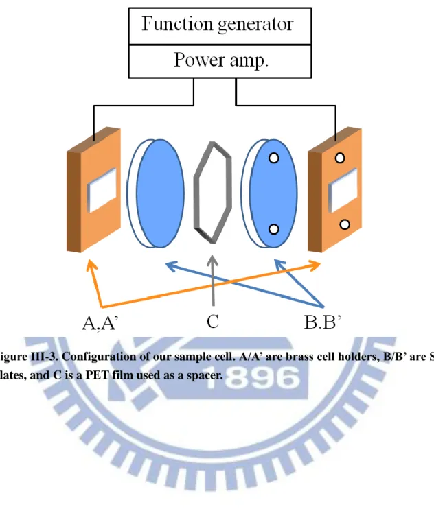
The configuration of our sample cell is schematically shown in Fig. III-3. The sample cell consists of a brass cell holder (A/A’), two Si windows (B/B’) and a polyethylene telephthalate (PET) thin film (C) as a spacer. The PET film (Diafoil®) was a gift from Mitsubishi Plastics. The Si windows (Pier Optics) used were p-type boron doped Si plates (resistivity = 0.8–2 Ω cm), so they also serve as electrodes. Because one side of the Si window was coated by a SiO2 layer (thickness = 0.3 μm, resistivity >1010 Ω cm),
the electrodes were electrically insulated from the sample. The resulting transmission of the Si plates is about 60% in the mid-IR region. The thickness of the PET film must be thin enough to avoid using high voltages, and a 6 μm film was our choice of the spacer. Between A’ and B’, we put chemically durable perfluoroelastmer O-rings (As568A-008) to prevent a liquid sample from leaking out of the flow system during measurement. Flowing the sample was required in order to avoid sample evaporation.
Accurate estimation of the cell gap and the applied voltage is essential for calculating the external electric-field strength. We can estimate an actual cell gap from an interference fringe pattern that appears in the absorption spectrum of the vacant cell. The peak positions of two adjacent peaks of an interference fringe pattern, ω1 and ω2 (cm−1),
are related to the cell gap a (μm) as
2 1 2 10 2 1 4 1 m a n (III-1)
2 1 2 10 2 2 4 2 m a n (III-2)
Where are refractive indices at ω1 and ω2, respectively, and m is an integer.
Assuming that
1 2
ω ω
n n , the cell gap a is obtained as
1 2 4 10 2 1 ω ω a (III-3)
In order to suppress unwanted work at the cell caused by non-zero resistance between A-A’ (VAA’) and B-B’ (VBB’), we need to make the contact resistance between
them as small as possible. To that end, we scratched the SiO2 uncoated surface of the Si
plate at two points with a distance of ~2 cm to physically remove the naturally coated SiO2 layer. On those points was pasted indium gallium alloy (Ga 40%), making electric
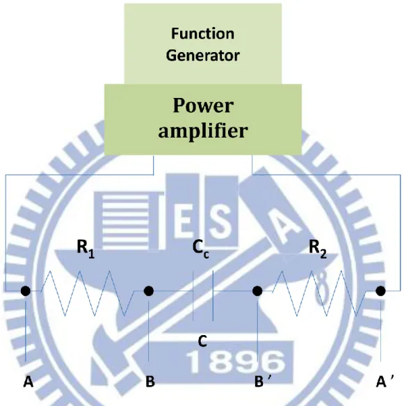
contacts with the brass cell holder. The resistance between the two points was nominally smaller than ~20 Ω. It depends upon doping properties of the Si plates. A large resistance may give rise to a decrease in amplitude of the applied voltage and phase retardation with respect to the applied sinusoidal wave. The latter may result in nonzero out-of-phase ΔA signals. This phenomenon has been explained by regarding the sample cell as forming an RC circuit. Fig. III-4 shows an RC circuit equivalent to the sample cell. R1 and R2 are the resistances between A and B and between A’ and B’, respectively. Cc is the capacitance between the electrodes. The exact voltage across the sample (VBB’) is related to the
applied voltage (VAA’) as [12]
2 2 2 1 i 1 1 1 1 c c c c A A B B RC RC RC RC V V (III-4)where RR1R2, і is the imaginary unit, ω is the angular frequency of the electric field
AA' 2 C Amplitude , 1 ( ) V RC (III-5)
Retardationarctan
RCc
(III-6) respectively. The capacitance CC changes depending on the dielectric constant of the sample. In the previously studies[17], the capacitance Cc rather than the resistance R is considered to be the main cause of the above problem.The magnitude of an externally applied electric field, Fext, can be calculated from
the applied voltage and the cell gap. However Fext is not the exact strength of the electric
field that is acting on molecules in the sample. It is the local field Flocal that is actually
exerted on the molecules [17]. Therefore, we need to consider the relation between local and external electric fields. The local electric field Flocal is related to the external field as
Flocal f f Fext (III-7) Here the factor given by
2 2 2 1 i 1 1 1 1 c c c c RC RC RC RC f (III-8)which accounts for the effect of the RC circuit that the sample cell may form, and f ’’ is the local-field correction. It is often very difficult to evaluate the factors f’ and f ’’ accurately, though they are of great importance in obtaining molecular properties, such as the dipole moment and polarizability, from ΔA signals. According to the Onsager theory, for instance, the local field correction is given by
r r 3 2 1 f (III-9)
unity to infinity, resulting in the value of f″ between 1.0 and 1.5. However, this theory is based on a simple model of intermolecular interactions and liquid structures, and there are many limitations to broad applications. Thus values of molecular properties are often quoted in units of f″ in previous studies [28, 29].
III-3. Sample preparation
To study the solvent effects on the trans–gauche conformational equilibrium, 1,2-dichloroethane (DCE) was mixed with four solvents with different polarity (cyclohexane, toluene, d-chloroform, and tetrachloromethane). Molecular sieves were added to DCE and solvents, followed by filtration (pore size = 0.2 μm), in order to remove residual water and dusts. Binary liquid mixtures of DCE and the four solvents at DCE mole fractions of 0.1, 0.2, and 0.4 were sonicated for 10 min by an ultrasonicator to confirm that the two liquids were mixed well.
III-4. Electroabsorption (A) and intensity difference (I) spectra
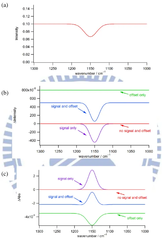
In this section, we would like to demonstrate how the presence of an offset in the I spectrum that is possibly caused by the electronics results in artifacts in the A spectrum. This effect raises a caution when the A spectrum is analyzed quantitatively. In Chapter II, we showed that the A spectrum is calculated from the I and I spectra according to Eq. II-1. Equation II-1 shows that the A signal depends not only on I but also on I. This fact may give rise to artificial peaks in the A spectrum even when there is no intensity change of an IR transition of the molecule induced by an electric field. Suppose that there is an absorption band at 1150 cm−1. It appears as a negative signal in the intensity (I) spectrum [Fig. III-5(a)]. Here, we consider four kinds of conditions [Fig. III-5(b)]: (i) Neither signal nor offset is observed, that is, I = 0 for all the wavenumbers (red spectrum). (ii) There is an absorption intensity change of −4.4 × 10⁻⁷ at 1150 cm−1
without any offset (purple spectrum). This is the ideal case. (iii) The I spectrum contains both constant offset of 5 × 10⁻⁷ and absorption intensity change of −4.4 × 10⁻⁷ at 1150 cm−1 (blue spectrum). (iv) The I spectrum contains a constant offset of 8 × 10⁻⁷ only (green spectrum). Unfortunately, we sometimes encounter cases (iii) and (iv), producing an unwanted distortion of the spectrum or emergence of an artifact.
For each of the four cases, we simulated the A spectrum using Eq. II-1. The resulting A spectra are shown in Fig. III-5(c). In case (i), there is no feature at all in the
A spectrum. In case (ii), a positive peak is observed at 1150 cm−1, which is the true signal we want to obtain. In case (iii), a positive peak is still seen on top of an offset of ~2 × 10⁻⁶. It should be noticed, however, that the peak height at 1150 cm−1 is somewhat diminished compared to that in case (ii). Furthermore, the peak at 1150 cm−1 accompanies tiny dips at both edges. These features seen in the A spectrum have nothing to do with molecular responses because the corresponding I spectrum shows no such features. What is worse, the A spectrum in case (iv) exhibits a negative peak of similar amplitude at 1150 cm−1. Obviously, this negative peak is a false signal; there is no absorption intensity change in the I spectrum [see Fig. III-5(b), green line].
The simple simulation demonstrated above gives an important caution: if one does not monitor the I spectrum and focus exclusively on the A spectrum, one may misinterpret the A signal containing an artifact that originates from an offset in the I spectrum and hence reach an erroneous conclusion regarding the electric-field effects on the molecule. Therefore, it is crucial to confirm that the I spectrum shows intensity changes at vibrational transition frequencies before interpreting the A spectrum.
Figure ΙIΙ-3. Configuration of our sample cell. A/A’ are brass cell holders, B/B’ are Si plates, and C is a PET film used as a spacer.
Figure ΙIΙ-4. RC circuit equivalent to the sample cell (Fig. ΙΙΙ-3.). R1 is the resistance
between A and B, R2 is that between A’ and B’, and Cc is the capacitance of the
Figure ΙIΙ-5. (a) Intensity spectrum. (b) I spectra with neither signal nor offset (red line); with signal only (purple line); with both signal and offset (blue line); and with offset only (green line). (c) Corresponding A spectra simulated using Eq. II-1.
(b)
(a)
Chapter IV
Infrared Electroabsorption Spectroscopic Study
of the Solvent Effect on the Conformational
Equilibrium of Liquid 1,2-Dichloroethane
IV-1. Introduction
Solvent effects are a collective term describing the phenomena that chemical processes are influenced by the properties of solvents including the dipole moment, dielectric constant, and refractive index. Solvent effects show up in many ways: different solvents yield distinct solubility of a solute, distinct degree of solute stabilization, and distinct rates for chemical reactions. Shifts in chemical equilibria are one of such effects caused by the ability of a solvent to alter the stability of a solute dissolved in it. In other words, the equilibrium constant of an equilibrium can be altered by changing solvents. The equilibrium shifts toward the direction of the substance involved in the equilibrium which is more stable than the others. The stabilization of the reactant or product can occur through any kinds of non-covalent interactions with the solvent, such as hydrogen bonding, dipole–dipole interactions, van der Waals interactions, etc. The influence of solvents on the position of chemical equilibria was found in 1896 independently by Claisen, Knorr, Wislicenus, and Hantzsch [30-33].
Changing solvents can potentially cause substantial effects on a specific type of chemical equilibrium, that is, conformational equilibrium. Although the enthalpy differences between conformational isomers are usually small, a conformational equilibrium often shows large solvent effects due to considerable solvation enthalpies of dipolar solutes.
Internal rotation of a C–C single bond plays an important role in conformational equilibria. Ethane is a prototype for understanding internal rotation around a C–C single bond. The function V V0
13cos
well describes the potential energy of the internal rotation in ethane, where is the H–C–C–H dihedral angle. The structure of ethane changes between an eclipsed conformation ( = 0°, 120°, or 240°) and the more stable staggered conformation ( = 60°, 180°, or 300°). In ethane, the three staggeredconformers are isoenergetic. However, when C–H bond(s) is substituted, they are not equivalent any more. This situation is realized in 1,2-dihaloethanes CH2X–CH2X, where
X represents a halogen atom. 1,2-Dihaloethanes possess three stable conformers, viz., two gauche and one trans conformers (see Figure IV-1a). The rotational isomerism was first discovered in DCE (X = Cl) by Mizushima and co-workers in 1936 [34]. The trans conformer is of C2h symmetry without having a permanent dipole moment ( = 0 D),
whereas the gauche conformer is of C2 symmetry having a non-zero permanent dipole
moment ( = 2.55 D [35]). Because the two chlorine atoms are most distant from each other in the trans conformer, the minimum repulsion force makes the trans conformer most stable (see Figure IV-1(b)).
The trans/gauche equilibrium is characterized by the free energy difference ΔG between the two conformers. The enthalpy difference, H, of DCE has been experimentally determined to be 0.0 kJ mol−1[36]. The small enthalpy difference indicates that it is difficult to determine G through the temperature dependence of IR or Raman spectra. IR electroabsorption spectroscopy has proven itself a powerful alternative for experimental determination of ΔG. Hiramatsu and Hamaguchi [17, 19] used IR electroabsorption spectroscopy to determine the equilibrium constant K0 and the Gibbs free energy and entropy differences of pure DCE.
Because the trans conformer is nonpolar and the gauche conformer is polar, the two conformers of DCE would experience a different degree of stabilization when mixed with a solvent. More specifically, it is expected that in a polar solvent, the population of the trans conformer decreases, whereas that of the gauche conformer increases. This change in population ratio gives rise to the change in the G and S values. In other words, the values of G and S for DCE in different solvents sharply reflect the microscopic
IR electroabsorption spectroscopy to determine K0, G, and S of DCE mixed with various solvents possessing different polarity (d-chloroform, toluene, CCl4, and
cyclohexane). Through a thorough comparison of the thermodynamic parameters so determined, we discuss the intermolecular interactions between DCE molecules and solvent molecules as well as the correlation between the thermodynamic parameters and commonly used indices for solvent polarity including dipole moment, dielectric constant, and the ET(30) value[37].
IV-2. Analysis
Since an applied electric field interacts in a distinct manner with the non-polar trans conformer and the polar gauche conformers of DCE, it shifts the equilibrium between the two conformers. The equilibrium constant K0is related to the Gibbs free energy difference (ΔG) between the two conformers (i.e., ΔG = Gg − Gt) as
RT G N N K 0 2exp t 0 g 0 (IV-1)
where Ng0 and Nt0 denote the numbers (populations) of the gauche and trans conformers,
respectively, R is the gas constant, and T is the temperature. Note that the superscript 0 always represents a physical quantity in the absence of the electric field.
When the external electric field is applied, an additional energy G is introduced to G via the dipolar interaction between the local electric field F and the permanent dipole moment g, of an isolated gauche conformer. G is given by NAgFcos,
where NA is Avogadro’s constant and is the angle between g and F. The equilibrium
F g F F t A g 0 equ Δ δΔ 2 exp cos 2 exp exp cos N θ G G K θ N θ RT ΔG N F RT K (IV-2)where NgFt
θ denotes the number of the gauche or trans molecules that are oriented along the direction , and NAkB = R is used (kB is the Boltzmann constant). Here,equ gF k TB
is a parameter representing the electrostatic interaction for an isolated
gauche molecule, which is responsible for the gauche/trans equilibrium change.
The total number of the gauche conformers, N , in the presence of the electric gF field is calculated by
d sin 0 F g F t F g F g F t F g
N N N N N N (IV-3)
F gN is independent of and is equal to F t 2 1
N . Taking this into account, Eq. IV-3 yields
d sin 1 , 2 1 0 F F F g ori F t F g
K K N f N N (IV-4)with f
,
ori
being an anisotropy function of the form
exp cos exp exp , ori ori ori ori ori f (IV-5)Here ori is another electrostatic interaction parameter that causes rotational orientation.
F F 0
0 t 0
g N
N and NgF NtF . The absorbance change ratios for the gauche and trans conformers are then computed by
Δ
g tF g t0
g t0 g tF g t0 1g t
A A N N N N N . They
have the forms [17, 19]
1
6 1
6
1 equ ori 2 0 0 2 equ 2 0 g K K K A A (IV-6) and
6 1 6 1 1 equ ori 2 0 0 2 equ 2 0 0 t K K K K A A (IV-7)respectively. Here A is the absorbance of the band of interest.
It should be noted that the equilibrium constant K0 is directly obtained by taking the ratio of (A/A)t to (A/A)g. To put it in another way, it is the ratio of A/A between the
gauche and trans conformers that counts for determination of the thermodynamic parameters. They can be determined independently from the electrostatic parameters equ
and ori, which may often contain uncertainties due to the local field correction and the
dielectric constant in the liquid phase. We also note that, according to Eqs. IV-6 and IV-7, the equilibrium change signal appears as the zeroth-derivative component of the absorption band shape.
For the polar gauche conformer of DCE, the electric-field-induced orientational polarization contributes to the A signal. As derived in Chapter II, the A signal originating from orientational polarization is described by Eq. II-22. In addition, the electronic polarization also gives rise to the A signal, which is given by Eq. II-24. Consequently, the model functions with which to analyze the observed A spectra are
2 2 0 equ or equ 2 0 0 g population change 2 2 2 2 ori 2 2 2 orientional polarization electronic polarizati 1 6 1 6 1 1 3cos 12 15 30 i A K A K K B d A C d A F hc d h c d on (IV-8)for IR bands of the gauche conformer and
2 2 0 equ or equ 0 2 0 0 t population change 2 2 2 2 2 electronic polarization 1 6 1 6 1 15 30 i A K K A K K B d A C d A F hc d h c d (IV-9)for those of the trans conformer. Here we neglect the zeroth-derivative component of the electronic polarization because the equilibrium shift and orientational polarization are major contributions to the A spectra.
IV-3. Methods and materials
The experimental apparatus and the sample cell for IR electroabsorption spectroscopy used in this study have already been described in Chapter III.In measuring the A spectra, we used a photoconductive MCT detector. Eight runs were averaged to obtain each A spectrum, which took about 40 min to scan. We paid special attention to the sample flow through the cell unceasingly in order to prevent heat accumulation and solvent evaporation during measurements carrying out at room temperature. The mole fraction of DCE in binary mixtures, xDCE, was set to xDCE = 0.2 in binary mixtures. FT-IR spectra
were recorded on with a JASCO FT/IR-6100 spectrometer using a sample cell composed of two CaF2 windows and a lead spacer (50 μm thick). Resolution of 8 cm−1 was used.
1,2-Dichloroethane (DCE) (>99.9%) was commercially obtained from J.T Baker; cyclohexane (>99.5%) from ACROS; toluene (>99.7%) from Sigma-Aldrich; d-chloroform (>99.8 atom % D) from Sigma-Aldrich; tetrachloromethane (>99%) from ACROS. Those chemicals were used as received. The dipole moment, dielectric constant, and the ET(30) value of each solvent are summarized in Table IV-1. Here, we used
d-chloroform instead of normal chloroform because several absorption bands of normal chloroform overlap with those of DCE. Deuterated and normal chloroforms are similar in terms of polarity: for example, both have the same dielectric constants of 4.8[38] and similar dipole moment (1.01D[39] for d-chloroform vs. 1.02D[40] for normal chloroform). All the experiments were done at room temperature (298 K).
IV-4. Results and discussion
IV-4-1. FT-IR spectra of pure DCE and binary mixtures of DCE
Figure IV-2 shows the FT-IR spectra of pure DCE and four binary mixtures of DCE and cyclohexane, CCl4, toluene, and chloroform at mole fraction xDCE = 0.2 in the
1360–1150 cm−1 region. Three IR absorption bands are observed in Fig. IV-2(a). The two bands at higher wavenumbers are assigned to the CH2 wagging mode of the gauche
conformer with different symmetry species a and b, and the lowest-wavenumber band is assigned to that of the trans conformer (see Table IV-2) [18]. From Figure IV-2(a), we can see that the trans band shows similar absorbance, whereas the gauche a and b bands show absorbance decreasing on going from polar to nonpolar solvent. In order to facilitate comparison, the spectra are normalized to the peak height of the trans band. The normalized spectra (Figure IV-2(b)) shows that the intensity ratio of the gauche bands to the trans band decreases as the solvent changes from polar to nonpolar. This change is a clear manifestation of the solvent effect on the conformational equilibrium of DCE. It is important to note, however, that the normalized FT-IR spectra of DCE mixed with toluene