以狀態轉換之Copula模型做動態資產配置 - 政大學術集成

全文

(1) 國立政治大學風險管理與保險研究所碩士學位論文 . 政治大指導教授：黃泓智博士立. ‧ 國. 學. 王昭文博士 . ‧ er. io. sit. y. . Nat. . . n. a. v. l CCopula 模型做動態資產配置以狀態轉換之 ni. hengchi U. Dynamic Asset Allocation with Regime-switching Copula . 研究生孫博辰中華民國一百零一年七月 .

(2) 謝辭時光飛逝，研究所生涯瞬間便到了尾聲，對於跨領域就讀的我來說，這兩年獲得的成長實在是相當充實。首先，要感謝的就是我的指導教授黃泓智老師，與王昭文老師。黃泓智老師在這一年中給了我許多關於學術與實務的教導，跟著老師做研究案也讓我從中汲取許多經驗，著實令我獲益良多；昭文老師對於我論文模型的建立、方向均細心給予指導，學到了相當多不同的研究領域知識。雖然在口試之前論文仍未臻完善，但還是在老師們的幫忙下完成了初稿，最後也感謝楊. 政治大. 曉文老師、楊尚穎老師於口試時提出的建議和意見，使我的論文成果更加完整。. 立. 研究所這兩年時間，認識了許多好同學們，無論是為了報告交互討論、或是. ‧ 國. 學. 共同出遊玩樂，都必是我最珍惜的回憶。尤其是精算組的同學們，分享對於未來. ‧. 的憧憬、一起為了考試而奮鬥努力，彼此間的信賴總能令有時苦悶的生活更添樂. y. sit. io. er. 標而努力。. Nat. 趣，也希望在未來的職涯中，大家都能維持感情、互道近況，各自追尋自己的目. al. n. v i n Ch 最後，衷心感謝家人與朋友們的支持與陪伴，對於我的選擇與決定總是予以 engchi U. 完全的支持與肯定，才讓我可以一路完成了碩士學業，是我在求學過程中永遠的動力，感謝你們的包容與鼓勵。謹將此文獻給最摯愛的你們。. 孫博辰. 謹誌於. 國立政治大學風險管理與保險學研究所中華民國一百零一年七月 . .

(3) 摘要. 在國際間的股票市場中，股票報酬常存在有不對稱的相關結構，而其會造成許多極度地尾端風險。Copula 函數常被用來描述多變數之間的聯合相關程度。多數的文獻均以二元 copula 函數為架構，去描述多種不同資產，像是股票、債券、匯率等之間的關係。我們討論多元 copula 的應用，本文以四元 copula 為主軸，並輔以狀態轉換 (regime-switching) 之機率過程，建構出四資產的投資組合之相關結構模型。. 政治大在模擬過程中，我們嘗試根據不同的未來目標做出最佳的投資組合權重，並採用立考慮了狀態轉換之 copula 的配適性後，我們以此模型來做資產投資策略。. ‧ 國. 學. 動態預期模型 (dynamic anticipative model) 來藉由資訊的不斷更新，重新估計模型的參數來做資產評估。實證結果上，我們發現考慮狀態轉換之 copula 模型可. ‧. 以捕捉到更多股票報酬波動的情形，因此能減少在股市共跌時造成的重大損失。. sit. y. Nat. n. al. er. io. 關鍵字：資產配置，多元 copula，狀態轉換. Ch. engchi. . i n U. v.

(4) Abstract The correlation of returns in international stock markets exist asymmetric structure, which cause extremely tail dependence. The copula functions are commonly used to describe the dependence between random variables. Most literatures use basic pair-copulas to model the dependence of two variables, like stocks, bonds and exchange rates. This article try to use multivariate copulas, mainly 4-copula, and. 政治大. regime-switching method to construct a portfolio dependence, and extend to asset. 立. allocation.. ‧ 國. 學. Given the fitting regime-switching copula, we use the model to decide investment strategy. We try to select the optimal weights of portfolio by different. ‧. objective function, and we adapt a dynamic anticipative model, which can take all. y. Nat. io. sit. new information for parameters estimation. Empirically, we find that the copula-based. n. al. er. model with regime-switching can capture more variation, and decrease the return loss from downside co-movement.. Ch. engchi. i n U. v. Key word: asset allocation, multivariate copula, regime-switching. . .

(5) Catalog Catalog……………………………………………………………….……….…..……I List of Table…………………………………………………………………..…..…...II List of Figure………………………………………………………………..…..……III 1. Introduction…………………………………………………………………………1 2. Copulas: basic definition and concepts……………………………………………..3 2.1. Pair copula.......................................................................................................3. 治政 2.2. Multivariate copulas…………………………………………………………3 大立 2.3. Parametric families of n-dimentional copulas……………………………….4 ‧ 國. 學. 2.3.1 Symmetry copulas………………………………………………….…4 2.3.2 Asymmetry copulas…………………………………………………...5. ‧. 3. Copula model selection..............................................................................................7. y. Nat. 3.1 Marginal distribution………………………………………………………..7. io. sit. 3.2 Dependence structure.....................................................................................8. n. al. er. 3.3 Estimation…………………………………………………………………...9. i n U. v. 3.4 Portfolio selection…………………………………………….....................11. Ch. engchi. 4. Empirical analysis…………………………………………………………………14 4.1 The Data…………………………………………..………………………...14 4.2 Estimation of the marginal models………………………………………….15 4.3 Estimation of the copula models……………………………………………17 4.4 Simulation procedure for optimal portfolio asset allocation…......................24 5. Conclusion…………………………………………………………………………27 Reference………………………………………………………………......................28. I .

(6) List of Table. Table 1. Descriptive statistics of daily returns of stock indices………………………………………...15 Table 2. Parameter estimates of the ARMA(1,1)-GARCH(1,1) model with skewed-t distribution……16 Table 3. The parameter estimates of the one-state copula……………………………………………...18 Table 4. Parameter estimates of regime-switching copulas-based on Gaussian copula………………..19 Table 5. Parameter estimates of regime-switching copulas-based on Student-t copula………………..20. 政治大. Table 6. Commonly used one-parameter Archimedean generators…………………………………….25. 立. Table 7. The Fund values of the out-of-sample performance for the two objective. ‧ 國. 學. functions and three different models…………………………….…………………………26. ‧. n. er. io. sit. y. Nat. al. Ch. engchi. II . i n U. v.

(7) List of Figure Figure 1(a). Gaussian-Gaussian copula…………………………………………………………..…….21 Figure 1(b). Gaussian-Student-t copula…………………………………………………………..…….21 Figure 1(c). Gaussian-Gumbel survival copula……………………………………………………...…21 Figure 1(d). Gaussian-Clayton copula………………………………………………………………….22 Figure 2(a). Student-t - Student-t copula……………………………………………………………….22. 政治大 Figure 2(c). Student-t - Clayton立 copula………………………………………………………………...23. Figure 2(b). Student-t - Gumbel survival copula……………………………………………………….22. ‧. ‧ 國. 學. Figure 2. The simulation results of asset allocation……………………………………………………26. n. er. io. sit. y. Nat. al. Ch. engchi. III . i n U. v.

(8) 1. Introduction The correlation structure across financial markets has faced a lot of tremendous fluctuation. During the last few years, mainly from 2007 to 2010, several financial crisis induced lots of huge losses for many funds and investors. There is sufficient evidence that negative returns are more dependent than positive returns in international equity markets. Maximizing the returns is no longer the only target for investment. Because the probability of loss increases sharply, people start to pay more attention to risk management. In financial and economics, the asymmetry phenomenon in stock markets has. 政治大. been researched in various aspects. Ang & Chen (2002) give a test for asymmetric. 立. correlation based on conditional correlations. Ribeiro and Veronesi (2002) present that. ‧ 國. 學. there is a higher correlations between international stock markets during market downturns. Ang & Bekaert (2002a, 2002b) set a Markov switching model for. ‧. international returns and international asset allocation with two regimes respectively.. y. Nat. sit. Patton (2004) observes significant asymmetry evidence in the dependence of financial. n. al. er. io. returns both in the marginal distributions and in the dependence structure.. i n U. v. Aiming to obtain more efficiency for modeling lower returns correlation, lots of. Ch. engchi. papers use copulas to describe the integrated distribution between assets. In recent years, the most popular method for dynamic time-varying copula model is regime-switching copula. Patton (2006) tests a model for asymmetry exchange rate dependence between Deutsche mark and the yen with time-varying copulas. Pelletier (2006) decomposes the correlation matrix with Markov regime switching. Okimoto (2008) also use a Markov switching model to capture more asymmetry evidence. Chollete et al. (2009) model the international financial returns in G5 and Latin American with a multivariate regime switching. Garcia and Tsafack (2011) test the extreme comovement between equity and bond markets. Candido et al. (2012) use 1 .

(9) hidden Markov chain (MC) allowing the unobserved time-varying dependence parameter to vary according to both a restricted ARMA process and an unobserved two-state MC. Manner and Reznikova (2012) generally provide a survey on various time-varying copulas. Definitely, there are many methods for optimal asset allocation strategy. There are two main methods of asset allocation. The first one is anticipative model. The anticipative strategy does not take account of future observations, and decides the investment strategy at decision date, by Blake, Cairns and Dowd (2001, 2003), Huang (2010), Huang & Lee (2010). The second method is adaptive model, which can take. 政治大. all new information for future strategy, as dynamic control (e.g., Haberman & Vigna,. 立. 2002, Jangmin et al., 2006, Emms & Haberman, 2007). Due to the difficult to acquire. ‧ 國. 學. closed form solution, the application of dynamic control still exist some limitations. The first and also the most important is a suitable multivariate model. Most of these. ‧. models are based on Brownian motions, but that cannot capture stock market. y. Nat. sit. downturns. A powerful technique to solve the problems is stochastic time-changing.. n. al. er. io. No matter what categories the model belongs to, fitting and modeling with time is. i n U. v. absolutely essential. Luciano and Schoutens (2006) consider a common gamma. Ch. engchi. process with two independent Brownian motion, Cont and Tankov (2004) proposed a bivariate correlated Brownian motion. In our paper, we use the regime-switching copula set a multivariate dependent model , and capture time-changing information, especially the lower tail risk. Huang (2010) propose the model that use multi-period anticipative concept to enhance the dynamic effect. According to the empirical results, we find that our model can capture more possible risks, and select optimal weights of the portfolio to get better returns.. 2 .

(10) 2. Copulas: basic definition and concepts In this article, we focus on the dependence of 4 assets portfolio. Except Gaussian and t copula, other copula functions, mainly Archimedean copulas, do not have a general multivariate distribution function. Umberto et al. (2004, 2012) explain complete and explicit copula methods in finance and more application. For capturing the asymmetric risks, we induct the 4-copulas p.d.f. and c.d.f which can get tail dependence of the data, and we use copula sampling method to generate random variables for simulation.. 2.1. Pair copula. 政治大. 立. By Sklar(1959), a pair copula is a joint distribution functions of standard uniform. ‧ 國. 學. random variables:. ‧. (2.1). y. Nat. where v, z  [0,1].. C (v, z )  P (U1  v, U 2  z ). er. io. sit. So from probability theory, that the probability-integral transforms of the r.v.s X and Y, are distributed as uniform:. n. al. i UC F ( X ), U  F (Y ) n hengchi U 1. 1. 2. v. 2. And we can use copula to give a joint function at (x, y):. F ( x, y )  P( X  x, Y  y )  C ( F1 ( x), F2 ( y )). (2.2). 2.2. Multivariate copulas According to Schweizer and Sklar (1983), an n-dimentional copula n C (u1 , u2 ,..., un ) is a multivariate distribution function in [0,1] :. F ( x1 , x2 ,..., xn )  C (u1 , u2 ,..., un )  C ( F1 ( x1 ), F2 ( x2 ),..., Fn ( xn )). and we can write the joint density function of the n-dimentional variable X as. 3 . (2.3).

(11) n. f ( x1 , x2 ,..., xn )  c(u1 , u2 ,..., un )   f i ( xi ). (2.4). i 1. where f i denotes the density function of variable xi . By the concepts of n-dimentional copulas, we can use them to describe the correlation between the variables, some like assets. Obviously, the result of copula fitted is effected by which copula we choose. For different kind of assets, we can select appropriate copula expected to display the correct data information.. 2.3. Parametric families of n-dimentional copulas. 政治大 most we care about is the downside co-movement between assets. Regarding to above 立 In this article, we aim to get suitable weight of asset allocation by copulas. The. section, we are going to present several common families of copulas, which include. ‧ 國. 學. symmetry ones, and tail dependence ones. We introduce main copulas used below:. sit. io. al. n. 2.3.1 Symmetry copulas. . C (1   ,1   ,1   ,1   )  1 1 .  U  lim. er.  0. ,. a). Gaussian copula. y. C ( ,  ,  ,  ). Nat.  L  lim. ‧. P.S. Tail dependence:. Ch. engchi. i n U. v. The Gaussian copula is defined by the cdf CRGA (u1 , u2 , u3 , u4 )   R   1 (u1 ),  1 (u2 ),  1 (u3 ),  1 (u4 ) . and the pdf by cRGA (u1 , u2 , u3 , u4 ) . 1 R. 1/ 2.  1  exp    T ( R 1  I )    2. 1 1 1 1 where     (u1 ),  (u2 ),  (u3 ),  (u4 )  . T. Gaussian copula has no tail dependence and its dependence parameter R is the correlation matrix. 4 .

(12) b). Student-t copula The Student-t copula is defined by the cdf CRt , (u1 , u2 , u3 , u4 )  tR ,  tR1 (u1 ), t R1 (u2 ), tR1 (u3 ), t R1 (u4 ) . and the pdf by  n. n. .   n       1  2      1   T R 1    1/2  2  2     cRt , (u1 , u2 , u3 , u4 )  R  1  1        2 4 2           i  2    2    1     i 1 . 政治大. 1 1 1 1 where    t (u1 ), t (u2 ), t (u3 ), t (u4 )  . T. 立. Student-t copula, some like Gaussian copula, has a correlation matrix coefficient R,. ‧ 國. 學. and a degree of freedomν. Specially different from the Gaussian copula, it shows some symmetry tail dependence.. ‧ y. Nat. n. al. er. Gumbel Copula. io. a). sit. 2.3.2 Asymmetry copulas. The Gumbel copula is defined by the cdf. Ch. engchi. i n U. v. 1/   4   C G (u1 , u2 , u3 , u4 )  exp     (  ln ui )       i 1. and the pdf by 4. cG (u1 , u2 , u3 , u4 )   i 1. ( ln ui ) 1 G  C (u1 , u2 , u3 , u4 )  ui. 4/  4 3/  4  4   4    6(  1)   ( ln ui )     (  ln ui )    i 1    i 1.  4  (  1)(11  7)   ( ln ui )   i 1 . 2/  4. 1/  4.  4   (  1)(2  1)(3  1)   ( ln uu )   i 1 . 5 .   .

(13) The Gumbel copula has only upper tail dependence. So as we need, we use the Gumbel survival copula which is be rotated 180 degrees and have the same pdf as before: c G (u1 , u2 , u3 , u4 )  c G (1  u1 ,1  u2 ,1  u3 ,1  u4 ). and it has only the tail dependence.  U  0,. b). i 1/  n     1  i  4  6  21/  4  31/  41/  ni   L  n 1  n  1  i 1/ 3  3  21/  31/  i1  n  1  i   1  i . . Clayton copula. 立. n. i 1. 政治大. c (u1 , u2 , u3 , u4 )  (1   )(1  2 )(1  3 ) u C. Nat.  ( 1) i.  4    ui  3  i 1 . n. U. L. ,.  n     n 1 . 1/. 4   3. engchi. er. io. which has only upper tail dependence. a l  0,  Ch.  (1/  4). sit. i 1. ‧. 4. 1/. y.  4  C C (u1 , u2 , u3 , u4 )    ui  3  i 1 . 學. and the pdf by. ‧ 國. The Clayton copula is defined by the cdf. 1/. i n U. v. The copula distribution we refers above have different characters, and the tail dependence is helpful to describe the data correlation. Due to the various functions, we can select adequate copula to fit as the joint distribution function of financial data. In this paper, we focus on the risk control and want to avoid big loss for our fund value, so we expect to obtain higher value by copula models.. 6 .

(14) 3. Copula model selection Our model aims to capture the type of asymmetric dependence found in international equity and bond markets. For asset allocation, we need to reduce the fluctuations in invested assets, especially downside co-movement. By means of regime-switching copula, we want to distinct more fluctuations in indices to maximize the portfolio returns. Therefore, we need to allow for asymmetry in tail dependence, regardless of the possible marginal asymmetry or skewness. Copulas, also known as dependence functions, are an adequate tool to achieve this aim. And simultaneously, for marginal. 政治大. distribution of asset returns, we also try to obtain the evidence of asymmetry.. 立. ‧ 國. 學. 3.1 marginal distribution. It ‘s well known that the residuals obtained from a GARCH model are generally. ‧. non-normal. This observation has exposed possibility of fat-tailed distribution.. y. Nat. sit. Hansen(1994) proposed a new density to model the GARCH model residuals, which. n. al. er. io. is a extension of the Student-t distribution with skewed factors. The Hansen’s skewed Student-t distribution is defined by. Ch. engchi.  1  2  2   bz a 1     bc 1    2  1        d ( z; ,  )    1 2  2    bz a 1    bc 1       2  1     . i n U if. v. z  a / b. (3.1) if. z  a / b. where  1 a  4 c ,  1. b 2  1  3 2  a 2 ,.  1    2  c ,    (  2)   2. and  and λ denote the degree-of-freedom parameter and the asymmetry parameter respectively. We will write Z~ST(  , λ) which means the random variable Z has the 7 .

(15) density d ( z; ,  ) . After the introduction of the residuals distribution, we continue to finish our models. For marginal distributions for the returns of given assets, we use ARMA(1,1)-GARCH(1,1)-Skewed-t model to fit asset returns: ri ,t  i  ai ri ,t 1  bi i ,t 1   i ,t ,  i ,t   i ,t zi ,t , i  1,..., 4.  i2,t  ki  pi i2,t 1  qi i2,t 1 zi ,t ~ ST (i , i ). (3.2). 2 The variables ri ,t represents the log returns of equity i ,  i ,t denotes the conditional. variances of ri ,t . The parameters of the marginal distributions are grouped into one. 政治大. factor   (1 ,...,  4 ) with  i   i , ai , bi , ki , pi , qi ,i , i  .. 立. ‧ 國. 學. 3.2 Dependence structure. Our dependence model is characterized by tow regimes, one the normal regime. ‧. ( st  1 ) corresponds to a symmetric dependence where the conditional joint normality. sit. y. Nat. can be supported, and a second regime assumed as a worse state ( st  0 ), corresponds. al. er. io. to the asymmetric regime in which markets are strongly more dependent for negative. v. n. returns than for positive returns. The conditional copula is given by:. Ch. F ( x1 , x2 , x3 , x4 )  C  u1 , u2 , u3 , u4 ; N ,  A | st . engchi. i n U.  st  C N  u1 , u2 , u3 , u4 ; N   (1  st )  C W  u1 , u2 , u3 , u4 ; A . where ui  Fi ( xi ) , and st  0, 1 is a state variable that follows a Markov chain process with a constant transition probability matrix as below.  P 1 Q  M  ; Q  1  P P  P ( st  1| st 1  1). and Q  P ( st  0 | st 1  0).. . In the previous chapter, we talk about a lot of copula functions. According to the variety features of these functions, we have several choices to fit our model. 8 . (3.3).

(16) Additionally, we will compare the fitness with no regime-switching copula to observe the improvement.. 3.3 Estimation The maximum likelihood method (MLE) could be very computationally intensive, especially in the case of a high dimension, because it is necessary to estimate jointly the parameters of the marginal distributions and the parameters of the dependence structure represented by the copula. Let us denote the observed data by T  { X 1 ,..., X 4 } where X t  { x1,t ,..., x4,t }. The log likelihood function is given by:. 政治大 L( , ;  )   log f ( X ;  ,  |  立 T. T. t 1. t. t 1. ). (3.4). ‧ 國. 學. Where   (  N ,  A , P, Q ) is the parameters grouped of the copula and the transition matrix. For the time series model of changes in regime, Hamilton(1989, 1994,. ‧. Chapter 22) presents a filter procedure to perform this kind of evaluation. With. Nat. n. al. Ch. er. io.  f ( xt ;  , | t 1 , st  1)  t     f ( xt ;  , | t 1 , st  0) . sit. y.   ( st ,1  st ) ', we denote the density function conditionally to the state variable st :. i n U. v. 4     c u , u , u , u ; | s 1 fi ( xi ,t ;  i )      t 1 2 3 4  i 1   4   c  u1 , u2 , u3 , u4 ; | st  0    fi ( xi ,t ;  i )  i 1  . engchi. (3.5). By the density function t , we can write the past returns as f ( X t ;  , | t 1 , st )  t 't. (3.6). and it can be integrated to a unconditional density function: 1. f ( X t ;  , | t 1 )   P( st  s | t 1;  , )  f ( X t ;  , | t 1 , st  s ). s 0. (3.7). The conditional probability, denoted by ˆt|t 1  [ P ( st  1| t 1 ;  ,  ), P ( st  0 | t 1 ;  ,  )]', 9 . (3.8).

(17) in different regime state can be computed by Hamilton filter. Given a starting value ˆ1|0 , the optimal inference and forecast for each date t in the sample can be found by. the following iterating equations:. ˆt|t . (ˆt|t 1  t ) 1'(ˆ   ) t |t 1. (3.9). t. ˆt|t 1  M  ˆt|t. (3.10). where ⊙ denotes element-by-element multiplication. Finally, the log likelihood function can be calculated of this algorithm:. 政治大 T. L( ,  ; T )   log f ( X t ;  ,  | t 1 ). 立. t 1. . T.   log ˆt |t 1t. ‧ 國. . 學. t 1. (3.11). Furthermore, from chapter 2, we know that the joint distribution density can be. ‧. written as a copula density product the margin density. According to the formula, the. y. Nat. log likelihood function can be written as. sit. n. al. where. er. io. 4 T   L( ,  ; T )   log  c(u1t , ..., u4t )   fi ( xi )  t 1 i 1   4. v.   Li ( i ; t )  Lc ( ,  ; T ). Ch. i 1. engchi. i n U. (3.12). T. Li ( i ; t )   log f i ( xi ,t ;  i | t ) t 1. T. Lc ( ,  ; T )   log fi ( xi ,t ;  i | t ). t 1. We see that the log likelihood function can be decomposed into two positive terms: one term involving the copula density and its parameters, and one term involving the margins and all parameters of the copula density. Because of the numerous parameters needed to estimate from marginal distribution and copula function, it is difficult to estimate all parameters at one step. For that reason, our 10 .

(18) structure allows for a two-step estimation method, proposed by Joe and Xu(1996), called inference for the margins or IFM:. 1.. As a first step, we estimate the marginal distribution’s parameters:. ˆ  arg max. 4.  L ( ;  ).   (1 ,..., 4 ) i 1. 2.. i. i. t. As a second step, given  , we estimate the copula’s parameters:. ˆ  arg max Lc ( , ; t )  . where  ,  represent the sets of all possible values of  ,  respectively. For the second. 政治大. step, René and Georges(2011) give a proposition of the decomposition of the copula’s. 立. log likelihood function.. ‧ 國. 學. 3.4 Portfolio selection. ‧. After we have estimated all parameters by two steps, we continue to decide the. sit. y. Nat. method how to choose the best weights for our portfolio. The fund invested by the. er. io. weights and asset returns are denoted by. a l F (t  1)  F (t )   w (t ) 1  r (t )i v (3.13) n Ch U i r (t ) are the weights and daily e n gt, wc(th) and where F(t) means the fund we hole at time n. 4. i 1. i. i. i. i. returns of every asset. Here we try to use two objective functions:. 1). Quadratic cost function : By Wang and Huang (2010), we consider the periodical targets at each time t,. where t = 1,…,n, where n is the last date. The target value hold at time t is F *(t  1)  F *(t )(1  r *(t )),. (3.14). where r *(t )  Max(rG , rm (t )) , rG is the guarantee rate, and rm (t ) is the minimum return of the four assets at time t. The target fund represent we can invest no worse than the 11 .

(19) target rate, such as risk-free rate, to satisfy we will have a reasonable return. The cost function at time t is defined as C (t )    F *(t )  F (t )     F *(t )  F (t )  , for t  1,..., n. 2. (3.15). The former part of the cost function is to control the final fund value, to reduce the risk of asset matching. The second part of the cost function is to hold the downside risk. The higher θ means the achievement of the fund final target is more important. The higher κ means we take more attention to the downside risk than the asset matching.. 政治大 Consequently, we can write the value function as: 立. We want to minimize the future cost to determine our weights per period.. V ( F t )  min E (G (t ) | F t ). ‧ 國. (3.16). 學. t. where G (t )   un t v n u C (u ) denote the discounting future costs, F t denote the. ‧. information we obtain until time t, and  t  {w( s ), s  t , t  1,..., n  1} represents the. sit. y. Nat. investment strategy of the future. By the objective function to control the future cost,. n. al. er. io. we can obtain an optimal weights for every period.. 2). Target volatility. Ch. engchi. i n U. v. For risk-control target, target volatility is one of the most popular methods that we can control the volatility and make the fund value have smaller fluctuation. For the purpose, we can fix our investment not to be so risky, and have a conservative decision. We restrict the volatility of fund to keep as the historical data, for maintaining the return stability.. 12 .

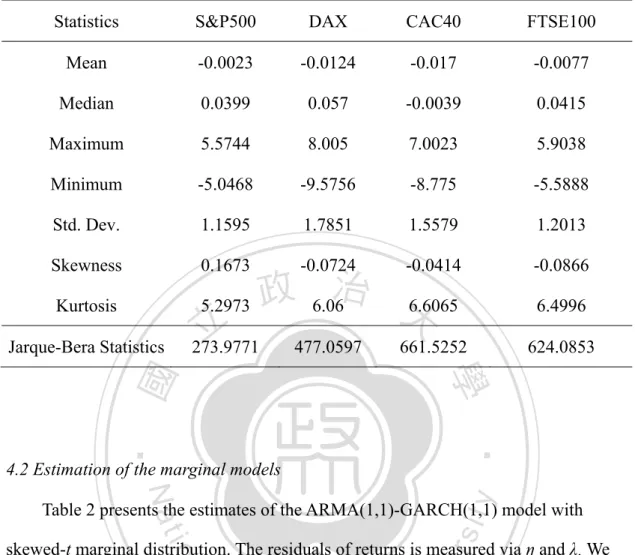
(20) 4. Empirical analysis. 4.1 The Data For general portfolio, we select four major stock indices as our assets. We employ the daily observations of S&P500, DAX, CAC40 and FTSE as proxy for target stock indices. The S&P500 index, which began from 1957, based on the common stock prices of 500 American companies. The DAX for the Deutsche Aktien Index, started from July 1, 1988, is a total return index of 30 selected German blue chip stocks traded on the Frankfurt Stock Exchange. The CAC40 for the French. 政治大. Cotation Automatique Continue Index, founded by December 31, 1987, represents a. 立. capitalization-weighted measure of the 40 most significant values among the 100. ‧ 國. 學. highest market caps on the Paris Bourse. FTSE100 for the Financial Times Stock Index, began on January 4, 1984, is a share index of the stocks of the 100 companies. ‧. listed on the London Stock Exchange with the highest market capitalisation. Our. y. Nat. sit. sample covers the period from January 1, 2001 to December 31, 2010.. n. al. er. io. Table 1 provides summary statistics on the selected stock market returns. The. i n U. v. period is from Jan 1, 2001 to Dec 31, 2005. We use the former five years to fit our. Ch. engchi. model to obtain initial parameters, and the latter five years to compare the returns that we simulated. From Table 1, we can see that S&P500 index has the lowest average daily returns and variance and DAX index has the highest daily returns and variance. In addition, all stock indices have significant non-zero skewness and positive excess kurtosis. The Jarque-Bera test is large and significant, that imply the assumption of normality is rejected.. 13 .

(21) Table 1. Descriptive statistics of daily returns of stock indices Statistics. S&P500. DAX. CAC40. FTSE100. Mean. -0.0023. -0.0124. -0.017. -0.0077. Median. 0.0399. 0.057. -0.0039. 0.0415. Maximum. 5.5744. 8.005. 7.0023. 5.9038. Minimum. -5.0468. -9.5756. -8.775. -5.5888. Std. Dev.. 1.1595. 1.7851. 1.5579. 1.2013. Skewness. 0.1673. -0.0724. -0.0414. -0.0866. Kurtosis. 5.2973. 立. Jarque-Bera Statistics. 政 6.06治大 6.6065. 273.9771. 477.0597. 6.4996. 661.5252. 624.0853. ‧. ‧ 國. 學. 4.2 Estimation of the marginal models. y. Nat. sit. Table 2 presents the estimates of the ARMA(1,1)-GARCH(1,1) model with. n. al. er. io. skewed-t marginal distribution. The residuals of returns is measured via η and λ. We. i n U. v. can observe that excluding FTSE100 index, the other three index have relative. Ch. engchi. significant degree-of-freedom η. For the asymmetry parameter λ, all stock returns have significant negative results. That means the skewed-t marginal distribution has preferable fitness.. 14 .

(22) Table 2. Parameter estimates of the ARMA(1,1)-GARCH(1,1) model with skewed-t distribution Parameters. S&P500. DAX. CAC40. FTSE100. C. 8.12E-05. 1.12E-03. 7.86E-04. 4.61E-05. (-0.8359). (1.8312). (1.4592). (1.6962). 0.6131. -0.9215. -0.8893. 0.8594. (2.3478). (-14.8262). (-11.4875). (14.0233). -0.6698. 0.8893. 0.8579. -0.9097. (-2.7257). (12.0435). (9.9349). (-18.6771). AR. MA. (1.4703). (1.5724). 0.0654. 0.0786. 0.0679. 0.0967. (4.1193). (5.4283). (5.0598). (5.7082). 0.9285. 0.9188. 0.9281. 0.8937. (54.5186). (64.5159). (69.5413). (51.2900). 19.4204. 16.7852. 13.2190. 45.7799. (2.3549). iv (3.2871) n U. (0.8590). -0.0644. -0.1718. n. λ. -0.0819. Ch. e n-0.1019 gchi. y. (2.2799). (-1.9855). (-2.5126). (-1.4754). (-3.9792). LLF. 3891.4768. 3471.5935. 3624.4153. 3974.4093. AIC. -3883.4768. -3463.5935. -3616.4153. -3966.4093. BIC. -3863.0504. -3443.1671. -3595.9889. -3945.9829. The value in the brackets is t-value of each variable.. 15 . sit. io. al. (2.1702). er. Nat ν. 9.36E-07. (1.4769). ‧. GARCH. 立. 治 8.07E-07 政9.26E-07 大學. ARCH. 6.63E-07. ‧ 國. K.

(23) 4.3 Estimation of the copula models For our copula models, we will compare the efficiency between single copula and regime-switching copula. Table 3 shows the estimates of the copula model which with no regime change. According to our assumption for four assets, the correlation matrix ρ has six parameters to be estimate. We can observe that Student-t copula has a larger LLF and the lower AIC/BIC, because of it can represent a little more tail dependence than Gaussian copula. The correlation matrix between the two copula model are nearly the same. All parameters are significant. Table 4 and Table 5 reports the parameter estimates of regime-switching copulas. 政治大. which based on Gaussian copula and Student-t copula respectively. We try seven. 立. different group, that the copula for state 1 is Gaussian or Student-t copula, the normal. ‧ 國. 學. state by our means, and the copula for state 2 have four copula as we introduce in chapter, which represent the worse state. Generally, all the regime-switching copulas. ‧. have much better fitness than one-state copula, because the higher LLF and lower. y. Nat. sit. AIC/BIC. Compared with Gaussian-based and Student-t-based copula, the latter. n. al. er. io. shows preferable results than the former. It’s because of that the Student-t copula can. i n U. v. capture a little more tail dependence. Especially, the best one of these groups are. Ch. engchi. Student-t to Student-t copula. We think it is due to the Gumbel survival copula and Clayton copula can only emphasize the lower tail dependence, almost all upper tail dependence cannot be categorized to them. So the effects of the lower tail dependent copulas are inferior to the t-t copula. Figure 1(a) to Figure 2(c) shows the copula correlation matrix by the estimated parameter.. 16 .

(24) Table 3. The parameter estimates of the one-state copula Gaussian ρ. Student's t. 0.5726. (31.0510). 0.5763. (31.4412). 0.4922. (12.3043). 0.5058. (20.2162). 0.4702. (10.9119). 0.4835. (18.9385). 0.8809. (27.8615). 0.8834. (59.8286). 0.7545. (19.3190). 0.7578. (34.1483). 0.8358. (63.3171). 0.8355. (66.4608). ν. 立. 政治 10.1663大. AIC. -1892.1342. -1935.5943. BIC. -1871.7081. -1915.1610. ‧ 國. 1943.5874. ‧. 1900.1345. 學. LLF. (3.8298). The value in the brackets is t-value of each variable.. n. er. io. sit. y. Nat. al. Ch. engchi. 17 . i n U. v.

(25) Table 4. Parameter estimates of regime-switching copulas-based on Gaussian copula State 1. Gaussian. State 2. Gaussian. P. 0.9621. (72.2967). 0.9286. (24.9906). 0.9311. (26.7870). 0.9851. (52.3512). Q. 0.9487. (44.2238). 0.9494. (32.3855). 0.4675. (1.9485). 0.6154. (3.6219). 0.6703. (4.1419). 0.7524. (4.2017). 0.5248. (20.9537). 0.5515. (23.8965). 0.5584. (4.1942). 0.6330. (4.8332). 0.4372. (14.2188). 0.4687. (12.2749). 0.5142. (4.4175). 0.5878. (11.6795). 0.4432. (9.8821). 0.8377. (31.4639). 0.8331. (10.8127). 0.8854. (50.8228). 0.8837. (39.0685). 0.6778. (14.6014). 0.7210. (12.1790). 0.7485. (27.6431). 0.7537. (20.8912). 0.8032. (14.9563). 0.8623. (6.4107). 0.8429. (56.8496). 0.8419. (64.2134). 2.7973. (3.0778). Student-t. Gumbel survival. Clayton. State 1. (8.4551). 0.4029. y. al. (9.6793). (9.4352). C h (9.1042) engchi 0.3939 (11.5986). 0.9400. (14.0210). 0.9187. (69.9711). 0.8621. (51.8244). 0.7884. (15.4843). 0.8807. (46.2354). 0.8191. (15.4039). 9.1851. (4.1144). ν. 0.4006. sit. (10.7613). er. 0.3932. 0.4384. n. (8.6002). 2.6114. io. 0.4281. ‧. Nat. alpha ρ. 治政 (6.8053) 0.4118 大. 學. State 2. 立. ‧ 國. ρ. i n U. v. LLF. 1959.4272. 1966.5813. 1922.4718. 1924.9460. AIC. -1945.4272. -1951.5813. -1913.4718. -1915.9460. BIC. -1909.6810. -1913.2818. -1890.4920. -1892.9662. The value in the brackets is t-value of each variable. 18 .

(26) Table 5. Parameter estimates of regime-switching copulas-based on Student-t copula State 1. Student-t. State 2. Student-t. P. 0.9832. (78.4811). 0.9846. (82.3797). 0.9941. (32.0426). Q. 0.9912. (178.8721). 0.6417. (2.8567). 0.7634. (1.9426). 0.3899. (8.5768). 0.5635. (29.3086. 0.5693. (23.7038). 0.3680. (8.7167). 0.4912. (19.5524). 0.4986. (10.0261). 0.3856. (10.3103). 0.4687. (18.2887). 0.4753. (9.0117). 0.8860. (35.8058). 0.7577. (21.0728). Gumbel survival. Clayton. State 1. 政 0.8861治 (63.1876) (117.7902) 大立 (22.1183) 0.7569 (35.4438). 0.9393. 0.8358. (66.2149). 0.8358. (66.1418). 31.4173. (3.5896). 10.3769. (4.6112). 10.3168. (2.8925). 2.4721. (15.1919). 0.6596. (4.1796). n. al. Ch. i n U. y. v. 0.5646. (4.3458). 0.5236. (4.9505). 0.8529. (24.3870). 0.7173. (4.0624). 0.8263. (5.5464). ν. 9.7811. (0.5830). LLF. 1990.4350. 1944.6560. 1946.5220. AIC. -1962.0340. -1934.6560. -1936.1580. BIC. -1928.7740. -1909.1230. -1911.3100. engchi. The value in the brackets is t-value of each variable. 19 . 2.5695. sit. io. ρ. (22.3328). Nat. alpha. 0.8596. ‧. State 2. 學. ν. ‧ 國. 0.8408. er. ρ. 0.9423.

(27) Figure 1(a). Gaussian-Gaussian copula. Figure 1(b). Gaussian-Student-t copula. 立. 政治大. ‧. ‧ 國. 學. n. er. io. sit. y. Nat. al. Figure 1(c). Gaussian-Gumbel survival copula. Ch. engchi. 20 . i n U. v.

(28) Figure 1(d). Gaussian-Clayton copula. Figure 2(a). Student-t - Student-t copula. 立. 政治大. ‧. ‧ 國. 學. n. er. io. sit. y. Nat. al. Figure 2(b). Student-t - Gumbel survival copula. Ch. engchi. 21 . i n U. v.

(29) Figure 2(c). Student-t - Clayton copula. 立. 政治大. ‧. ‧ 國. 學. n. er. io. sit. y. Nat. al. Ch. engchi. 22 . i n U. v.

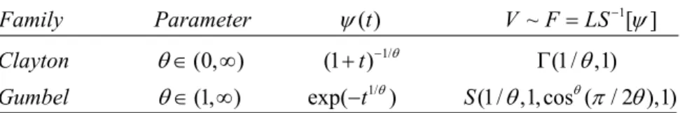
(30) 4.4 Simulation procedure for optimal portfolio asset allocation As we discuss in chapter 4.1, we take the estimated results as our simulation parameters, and contrast our results of investment strategy with historical data. According our model, we estimate the parameters of marginal distribution first, and continue to obtain the parameters of copula models. Considering that, we should start our simulation by copula sampling. By using the Matlab toolbox, we can easily sample multivariate Normal and Student-t copula, given the correlation matrix (and the degree of freedom for Student-t). For multivariate Archimedean copulas, we can use the following algorithm sampling Archimedean copulas, based on. 政治大. Laplace-Stieltjes transform, also known as the Laplace transform of the distribution,. 立. see Feller (1971, p. 439), Marshall and Olkin (1988), and Marius and Martin(2011). ‧ 國. 學. for advanced algorithms.. ‧. Algorithm of Sampling Archimedean copulas. y. Nat. V ~ F  LS 1[ ]. sit. (1) sample. n. al. er. io. (2) sample R j ~ Exp (1), j  {1,..., n} (3) set U j   ( R j / V ), j  {1,..., n} (4) return. U  (U1 ,..,U n ). T. Ch. engchi. i n U. v. By the algorithm, we can sample multivariate Archimedean copulas given the parameter α. Table 6 list the Laplace-Stieltjes transform of the Archimedean copulas used by our models. By sampling copula variables, we can get the marginal residuals to forecast future returns for every asset. To make our investment strategy more dynamic and efficient, we re-estimate all parameters of our model, select the best weights of portfolio, and re-assess the optimal investment at each decision date, assumed per four weeks here. 23 .

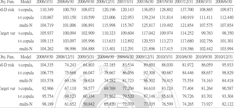
(31) Table 6. Commonly used one-parameter Archimedean generators Family. Parameter.  (t ). V ~ F  LS 1[ ]. Clayton.   (0, ). (1  t ) 1/. (1/  ,1). Gumbel. 1/.   (1, ). S (1/  ,1, cos ( / 2 ),1). exp(t ). Γ is the Gamma distribution, and S is the Stable distribution.. We first generate four weeks stock returns for each path by using the parameters of the model. In this paper, we simulate 10,000 stock return paths. Second, we choose the optimal weights for each asset given the predicted future returns for each path, and. 政治大. get the average weights of these 10,000 paths. Next, we take all new information for. 立. the historical data each decision date, to re-estimate the parameters for the new five. ‧ 國. 學. years data and repeat to acquire portfolio weight and fund values.. Figure 2 shows the results of asset allocation simulation from Jan 1, 2006 to. ‧. Dec13, 2010, and the empirical fund values are presented in Table 7. We assume the. Nat. sit. y. parameters   1,   1000 for quadratic cost function, and the other is target. n. al. er. io. volatility. We choose the Student-t copula and Student t-t regime-switching copula for. i n U. v. out-of-sample test, duo to they have larger log-likelihood value and lower BIC.. Ch. engchi. Simultaneously, we set a simple model that the four asset returns have a jointly multivariate Normal distribution. Obviously, the Student t-t copula has the outstanding result at all period. By given different state, regime-switching copula can avoid more financial loss than other models and obtain higher returns.. 24 .

(32) Table 7. The Fund values of the out-of-sample performance for the two objective functions and three different models Obj. Fun.. Model. 2006/3/31 2006/6/30 2006/9/30 2006/12/31 2007/3/31 2007/6/30 2007/9/30 2007/12/31 2008/3/31 2008/6/30. M-D risk t-copula,. 110.349. 100.793. 108.072. 120.196. 120.143. 136.053. 128.802. 137.700. 108.865. 109.871. t-t copula. 110.867. 103.150. 110.599. 123.006. 122.953. 139.234. 131.814. 140.919. 111.411. 112.440. multi-N. 104.719. 101.006. 106.891. 115.998. 115.767. 125.817. 119.492. 121.854. 107.575. 107.854. Target var t-copula,. 105.937. 100.094. 102.909. 110.323. 109.604. 117.042. 109.974. 114.252. 99.763. 98.350. t-t copula. 109.115. 103.097. 105.996. 113.633. 112.892. 120.553. 113.273. 117.680. 102.756. 101.301. multi-N. 104.262. 98.996. 104.888. 113.401. 112.291. 121.896. 117.415. 119.386. 102.442. 103.994. Obj. Fun.. Model. 2008/9/30 2008/12/31 2009/3/31 2009/6/30 2009/9/30 2009/12/31 2010/3/31 2010/6/30 2010/9/30 2010/12/31 104.335. 74.243. 64.803. t-t copula. 106.775. 75.668. 66.047. multi-N. 103.578. 69.156. Target var t-copula,. 92.966. 67.110. t-t copula. 95.754. multi-N. 98.189. ‧ 國. 58.624 立 58.577. 83.534 89.603 治政78.667 86.056 大92.308 74.282 81.723 86.302 77.185. 69.769. 77.204. 84.610. 88.030. 81.972. 86.059. 95.933. 90.687. 84.446. 88.657. 98.829. 79.415. 75.554. 74.163. 84.418. 83.124. 77.404. 81.264. 90.587. 學. M-D risk t-copula,. 69.123. 60.334. 71.862. 79.520. 87.148. 85.618. 79.726. 83.701. 93.304. 61.652. 50.842. 65.420. 72.079. 77.035. 76.599. 74.265. 73.927. 82.122. ‧. M-D risk is the cost function composed by matching risk and downside risk, and Target var is the target volatility. We choose the best performance copula model to simulate out-of-sample test. Excluding the. y. Nat. Student-t copula and t-t regime-switching copula, we also set a multivariate Normal distribution of. n. al. er. io. sit. assets to compare the results.. Ch. Figure 2. The simulation results of asset allocation. 150. engchi. i n U. v. t copula,M-D risk t-t copula,M-D risk Multivariate Normal,M-D risk t copula,Target var. t-t copula,Target var. Multivariate Normal,Target var.. 140 130 120 110 100 90 80 70 60 50 2005/12. 2006/06. 2006/12. 2007/06. 2007/12. 2008/06. 2008/12. 25 . 2009/06. 2009/12. 2010/06. 2010/12.

(33) 5. Conclusion In this paper, we propose a regime-switching copula-based model that can separate the equity returns to two regimes, a normal state that returns goes up and down by random, and a worse state that returns obviously have downside co-movement with large possibility. We capture the well-known phenomenon that there exists asymmetric behavior between international stock markets. By use of Hamilton filter, we can analyze the transition probability which provide sufficient about the current condition of markets. For asset allocation strategy, we use the model fitted by in-sample and simulate. 政治大. the future returns contrasted to out-of sample. We adapt “moving-window” method. 立. that makes our sample data can update per period, and re-estimate the parameters of. ‧ 國. 學. our model for fitting new information. The empirical results display that our model can decide optimal weights of portfolio, and we can avoid suffering huge loss in. ‧. financial crisis.. n. er. io. sit. y. Nat. al. Ch. engchi. 26 . i n U. v.

(34) Reference 1.. Ang, A. & Chen, J., 2002. Asymmetric correlations of equity portfolios, Journal. of Financial Economics 63(3), 443-94. 2.. Blake, D., Cairns, A. J. G., Dowd, K., 2001. Pensionmetrics: stochastic pension. plan design and value-at-risk during the accumulation phase. Insurance: Mathematics and Economics 29, 187-215. 3.. Blake, D., Cairns, A.J.G. & Dowd, K., 2003. Pensionmetrics II: Stochastic. pension plan design during the distribution phase, Insurance: Mathematics and Economics 33, 29-47. 4.. 政治大. O. Candido, F. A. Ziegelmann, J. Duekerc, 2012. Modelling the Dependence. 立. Dynamics through Copulas with Regime Switching, Insurance: Mathematics and. ‧ 國. 學. Economics 50, 346-356 5.. U. Cherubini, E. Luciano, W. Vecchiato, 2004. Copula Methods in Finence, The. ‧. Wiley Finance Series.. y. Nat. io. Methods in Finance, The Wiley Finance Series.. al. n. 7.. sit. U. Cherubini, S. Mulinacci, F. Gobbi, S Romagnoli, 2012. Dynamic Copula. er. 6.. i n U. v. L. Chollete, A. Heinen, and A. Valdesogo, 2009. Modeling international. Ch. engchi. financial returns with a multivariate regime switching copula, Journal of Financial Econometrics 7, 437-480. 8.. Garcia R. & Tsafack G., 2011. Dependence structure and extreme comovements. in international equity and bond markets, Journal of Banking & Finance Volume 35, 1954-1970. 9.. Haberman, S., Vigna, E., 2002. Optimal investment strategy and risk measures in. defined contribution pension schemes, Insurance: Mathematics and Economics 31, 35-69. 10. Emms P., Haberman, S., 2007. Asymptotic and numerical analysis of the optimal 27 .

(35) investment strategy for an insurermInsurance: Mathematics and Economics 40, 113–134. 11. Huang, H.C., 2010. Optimal Multi-Period Asset Allocation: Matching Assets to Liabilities in a Discrete Model, Journal of Risk and Insurance 77(2). 12. Huang, H.C. & Lee, Y.T., 2010. Optimal Asset Allocation for a General Portfolio of Life Insurance Policies, Insurance: Mathematics and Economics 46, 271-280. 13. Jangmin O., J. Lee, J. Lee, B. Zhang, 2006. Adaptive stock trading with dynamic asset allocation using reinforcement learning, Information Sciences 176, 2121–2147.. 政治大. 14. E. Jondeau and M. Rockinger, 2006. The copula-garch model of conditional. 立. dependencies: An international stock market application, Journal of International. ‧ 國. 學. Money and Finance 25, 827-853.. 15. E. Luciano & W. Schoutens, 2006. A multivariate jump-driven financial asset. ‧. model, Quantitative Finance 6(5), 385-402.. y. Nat. sit. 16. H. Manner & O. Reznikova, 2012. A Survey on Time-Varying Copulas:. n. al. er. io. Specification, Simulations, and Application, Econometric Reviews 31(6), 654-687. i n U. v. 17. A. Patton, 2004. On the out-of-sample importance of skewness and asymmetric. Ch. engchi. dependence for asset allocation, Journal of Financial Econometrics 2, 130-168. 18. A. Patton, 2006. Modelling Asymmetric Exchange Rate Dependence, International Economic Review 47, 527-556 19. A. Patton, 2009. Copula-based models for financial time series. In T. G. Andersen, R. A. Davis, J.P. Kreiss, and T. Mikosch, editors, Handbook of Financial Time Series. Springer Verlag, 2009. 20. D. Pelletier, 2006. Regime switching for dynamic correlations, Journal of Econometrics 131, 445-473. 21. Ribeiro, R. & P. VeronesiI, 2002. The Excess Comovement of International 28 .

(36) Stock Returns in Bad Times: A Rational Expectations Equilibrium Model, Working Paper. 22. T. Okimoto, 2008. New Evidence of Asymmetric Dependence Structures in International Equity Markets, Journal of Financial and Quantitative Analysis 43, 787–816 23. V. Zakamouline, S. Koekebakker, 2009. Portfolio performance evaluation with generalized Sharpe ratios: Beyond the mean and variance, Journal of Banking & Finance 33, 1242–1254.. 立. 政治大. ‧. ‧ 國. 學. n. er. io. sit. y. Nat. al. Ch. engchi. 29 . i n U. v.

(37)