A Tableless Approach for High-Level Power
Modeling Using Neural Networks
*CHIH-YANG HSU, WEN-TSAN HSIEH+, CHIEN-NAN JIMMY LIU+ AND JING-YANG JOU
Department of Electronics Engineering National Chiao Tung University
Hsinchu, 300 Taiwan
E-mail: {hsucy; jyjou}@eda.ee.nctu.edu.tw
+Department of Electrical Engineering
National Central University Taoyuan, 320 Taiwan E-mail: {wthsieh; jimmy}@ee.ncu.edu.tw
For complex digital circuits, building their power models is a popular approach to estimate their power consumption without detailed circuit information. In the literature, most of power models have to increase their complexity in order to meet the accuracy requirement. In this paper, we propose a tableless power model for complex circuits that uses neural networks to learn the relationship between power dissipation and input/ output signal statistics. The complexity of our neural power model has almost no rela-tionship with circuit size and number of inputs and outputs such that this power model can be kept very small even for complex circuits. Using such a simple structure, the neural power models can still have high accuracy because they can automatically con-sider the non-linear characteristic of power distributions and the effects of both state- dependent leakage power and transition-dependent switching power. The experimental results have shown the accuracy and efficiency of our approach on benchmark circuits and one practical design for different test sequences with wide range of input distribu-tions.
Keywords: power macromodel, power estimation, neural network, low power design,
RTL
1. INTRODUCTION
System-on-a-chip (SOC) is a trend of system integration in recent years. For SOC designs, most design teams will not design all circuit blocks in the system by themselves. Instead, they will integrate many well-designed circuit blocks called intellectual proper-ties (IPs) and some self-designed circuit blocks to build up the complex system in a short time. While designing such complex systems, power consumption is also a very impor-tant design issue because of the increasing requirement on operating time of portable devices. In order to avoid problems associated with excessive power consumption, there is a need for computer-aided design (CAD) tools to help in estimating the power con-sumption of very large scale integrated (VLSI) circuits, at various levels of abstraction. Received November 8, 2004; revised January 19, 2005; accepted March 23, 2005.
Communicated by Chung-Yu Wu.
A number of CAD techniques for power estimation at lower levels of abstraction, such as transistor-level [1-3] or gate-level [4], have been proposed. Generally speaking, they can provide more accurate estimation results. However, they may become unpracti-cal for complex designs because to simulate the whole design under such low levels re-quires too much computation resources. In addition, by the time the design has been specified down to gate level or lower, it may be too expensive to go back to fix high- power problems. Most importantly, IP vendors may not provide such low-level descrip-tion for an IP to protect their knowledge. Therefore, a number of high-level power esti-mation techniques [5-14] have been proposed to estimate the power consumption at a high level of abstraction, such as when the circuit is represented only by Boolean equa-tions. This will provide more flexibility to explore design tradeoffs early in the design process and reduce the redesign cost and time to fix power problems.
Those high-level techniques can be roughly divided into two categories: top-down and bottom-up. In the top-down techniques [6, 7], a combinational circuit was specified only as a Boolean function without information on the circuit implementation. Therefore, top-down techniques are useful when one is designing a logic block that was not previ-ously designed because they can provide a rough measurement about the trend of power consumption before implemented. However, they may not have very good accuracy due to lack of implementation details. For SOC designs, bottom-up approaches [8-14] are more useful when one is reusing previously designed circuit blocks such as IPs. Since all internal structural details of the circuit are known, they can build a power macromodel for this block to estimate its power consumption in the target system at function-level. Building those power macromodels often requires a power characterization process that uses low-level simulations of modules under their respective input sequences to record the relationship between high-level power characteristics and real power consumption. Because the power consumptions are measured in the low-level simulations with internal circuit information, the power macromodels can provide more accurate estimations than those in the top-down approaches. After the characterization step, no more low-level simulations are required in the estimation step. Users can obtain the power consumption of the circuits by only providing the high-level power characteristics obtained in func-tion-level simulations thus having a very fast estimation time.
Lookup table (LUT) is the most commonly used power macromodel. In order not to increase the table size too much, most of the LUT-based approaches [8-10] use the ag-gregate signal statistics (average input signal probability, average input signal transition density, average output signal transition density, input signal correlation coefficient, etc.) of the primary inputs and outputs of circuits to be the indexes of lookup tables. In [8], the lookup tables with 2 dimensions, 3 dimensions and 4 dimensions were compared. The results showed that the estimation errors are decreased when the dimensions of tables are increased, but the sizes of tables are also exponentially increased. For large circuits, the table size may increase very fast in order to meet the accuracy requirement.
The method in [11] built a one-dimension lookup table using the zero-delay charg-ing and dischargcharg-ing capacitance as table index. The authors proposed an efficient method to divide power characteristics of pattern pairs into several groups and fill the lookup table with the average power consumption of each group. Although this approach can build smaller lookup tables with reasonable accuracy, it still requires gate-level descrip-tions and node capacitance information to obtain the total charging and discharging
ca-pacitance in the circuits, which may not provided by IP vendors.
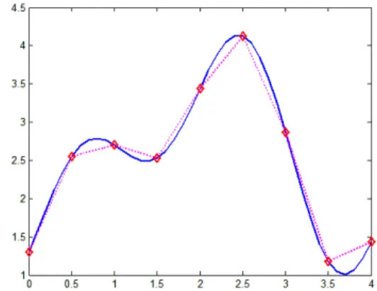
There are also some approaches [12-14] that use equations instead of lookup tables to be the power macromodels. After identifying suitable variables for the power equa-tions of a circuit, those equation-based approaches will use some numerical methods such as linear regression to find out the best parameter for each variable to form the equations. Compared to LUT-based approaches, equation-based approaches often have less data to be recorded for a power macromodel because the distribution of an equation often requires many points to describe. However, because the power distribution is often a very irregular curve as illustrated in Fig. 1, it is hard to use only a single equation to describe this curve. Therefore, in order to improve the accuracy of their power macro-models, those equation-based approaches may increase the order of the power equations (more variable) or use piece-wise power equations (more equations) to approximate the power distribution, which will significantly increase the complexity of the power mac-romodels.
Fig. 1. Irregular power distribution and piece-wise approximation.
Most of the above techniques focus on estimating the average power consumption over a long input sequence, which are referred to as cumulative power macromodels. However, in some applications, the average power is not sufficient. One of the other im-portant tasks is to understand the power consumption of a circuit due to a given pattern pair, which is often referred to as cycle-accurate power macromodels [13, 14]. This in-formation is crucial for circuit reliability analysis, dc/ac noise analysis, and design opti-mization. Of course, those cycle-accurate power macromodels can also provide the in-formation of average power consumption by just computing the average of the power consumed at each cycle in the given input sequence. Therefore, cycle-accurate power macromodels are considered to have more use than cumulative power macromodels. Be-cause it is not feasible to build a lookup table for every possible combinations at each cycle, most of those cycle-accurate power macromodels use equation-based approaches to record the power distributions.
In other research areas, neural networks play as a powerful tool in many applica-tions such as classification, clustering, pattern recognition, control application, etc. Be-cause of the self-learning capability of neural networks, they can recognize complex
characteristics by using several simple computation elements with proper training. For irregular distributions such as the power distribution shown in Fig. 1, neural networks can still have good efficiency because they use the combination of some non-linear curves to fit the multi-dimensional non-linear surface instead of increasing the recording points to reduce the errors as in the traditional power macromodels. Therefore, several researches [15, 18] tried to use neural networks to solve the power estimation problem. The authors in [15] proposed a symbolic neural network model to estimate the power consumption of circuits. Based on Hopfield neural network [16], they built another rep-resentation for the gate- level description of circuits and stored the structure information of the neural networks in algebraic decision diagrams [17] to reduce the memory usage. In that approach, neural networks were only used to replace the gate-level structures and to perform a gate-level simulation for estimating the power consumption of circuits with fewer resources. Therefore, the simulation time was only similar to the gate-level simula-tion, which will be very slow for large circuits.
The authors in [18] proposed a power modeling approach for library circuits using Bayesian inference and neural networks. They divided the leakage and switching power distributions of circuits into a limited number of classes and trained two neural networks to classify an input state or transition into the corresponding class. After classified, the leakage power of an input state and the switching power of an input transition can be estimated by the average power consumption of that class, which has been stored in a lookup-table as in the traditional table-based approaches. Although the classification of an input state or transition can be more accurate by using neural networks, the number of classes may limit the accuracy of this power modeling approach over the entire power spectrum. Therefore, they may also have to increase the number of table entries to reduce the estimation error, which is similar to the problem of traditional table-based approaches. In addition, if the table entries are increased, the number of outputs of the neural net-works is also increased. If there are too many outputs in a neural network, it will often become much harder to converge and sacrifice the classification accuracy. However, the authors did not show the experimental results for the cases with wide power distribution and large number of classes.
In this paper, we propose a quite different approach for high-level power modeling of complex digital circuits that uses a 3-layer fully connected feedforward neural net-work [19] to learn the power characteristics during simulation without any lookup tables. By considering all possible types of state transitions separately in the input data, both the state-dependent leakage power and transition-dependent switching power are still re-corded well in our power model. In addition, because the numbers of input and output neurons in our neural power model are fixed as 8 and 1 respectively, the complexity of our neural power model has almost no relationship with circuit size and the numbers of primary inputs and outputs such that this power model can be kept very small even for complex circuits. Unlike the piece-wise equations in the equation-based approaches, only one simple neural model is enough for those test circuits to provide similar accuracy thus reducing the modeling complexity.
The rest of this paper is organized as follows. The feedforward neural network and our neural power model will be described in section 2. In section 3, we will explain the details to build a neural power model. Finally, the experiment results will be demon-strated in section 4 and some conclusions will be given at the end.
2. BACKGROUND
2.1 Feedforward Neural Networks
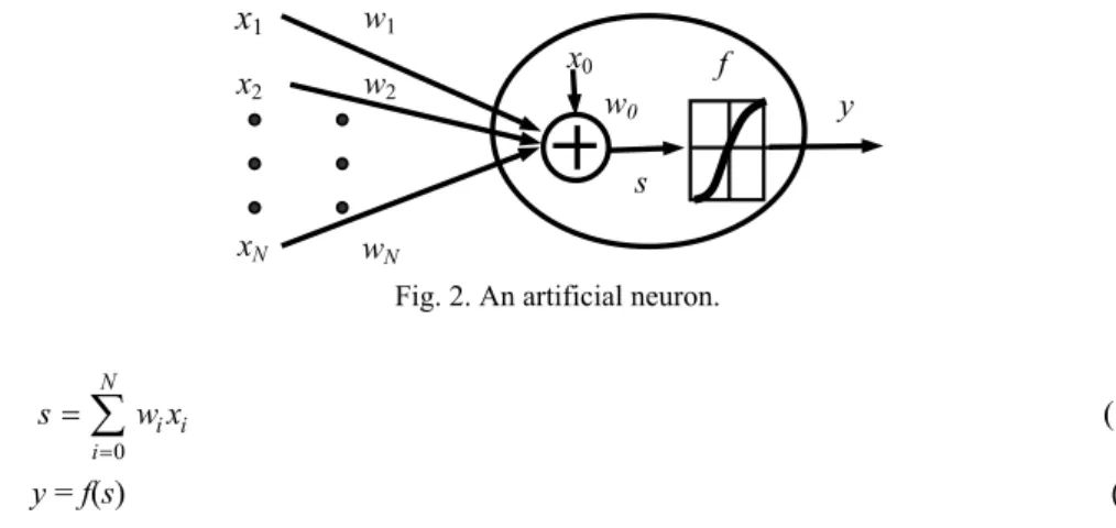
The basic unit in a neural network is an artificial neuron as shown in Fig. 2. In Fig. 2, x1 to xN are the input data for the neuron, w1 to wN are the weights of input x1 to xN
in-dividually that represent the contribution from each input, and s is the summation of x1w1 to xNwN and the bias factor x0w0 as represented in Eq. (1). In most cases, x0 is fixed as 1
such that the training algorithm only adjusts the weight w0 to wN. Function f is the
trans-fer function that converts s into output y as represented in Eq. (2). According to the rela-tionship between of input data and output data, users can choose different transfer func-tion f for each different case.
y
x
1 x2 xN w1 w2 wN f s w0 x0Fig. 2. An artificial neuron.
0 N i i i s w x = =
∑
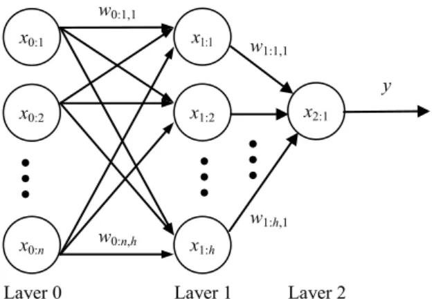
(1) y = f(s) (2)A neural network is a set of interconnected neurons, where the outputs of neurons act as the inputs of other neurons or the final outputs of the neural network. Feedforward neural network [19] is one of the most popular models of neural networks. Although any architecture of neural network with learning capabilities can be used in this work, we use the 3-layer fully connected feedforward neural network, as shown in Fig. 3, to learn the relationship between power consumption and statistic information of input patterns be-cause the 3-layer feedforward neural network has a quite simple structure with good per-formance in many applications. In addition, the fully connected configuration can auto-matically consider the correlation between all inputs by properly adjusting the weights for their interconnections. The accuracy of this power model can thus being improved because the correlation is also an important factor that affects power consumption.
In Fig. 3, xl:i represents the ith neuron in the lth layer, wl:i,j represents the weight of
the interconnection between neuron xl:i and xl+1:j, and y is the final output of this neural
network. The number of input neurons is n and the number of hidden neurons is h. In
order to simplify the graph, the biases, the summations, and the outputs of all neurons are
not labeled in Fig. 3. The weight of the bias in neuron xl+1:j is denoted as wl:0,j, the input
of the bias in neuron xl+1:j is denoted as al:0, the summation s in neuron xl:i is denoted as
sl:i, and the output of neuron xl:i is denoted as al:i. The output y in this neural network,
x0:1 x0:2 x1:1 x1:2 x1:h x2:1 x0:n y w0:1,1 w1:1,1
Layer 0 Layer 1 Layer 2
w0:n,h
w1:h,1
Fig. 3. A fully connected 3-layer feedforward neural network.
2:1 2:1 1: ,1 1: 0 ( ) h i i i y a f s f w a = ⎛ ⎞ = = = ⎜ ⎟ ⎝
∑
⎠ (3) If we are going to use neural networks for high-level power estimation, we have to decide the input data type, the number of hidden neurons and the transfer function of internal neurons to build up a suitable neural network structure for our application. We will discuss the details of our decision strategies for those parameters in section 3.2.2 Training Process
Before using a neural network, we have to train the neural network with proper strategies such that it can learn as many experiences as it needs. Given a 3-layer neural network η with N input neurons, H hidden neurons and 1 output neuron, we can denote the training set as T = {(xi, ti), i = 1:P}, where xi is a column vector of the ith input vector,
ti is the expected output for the ith input vector, and P is the size of training set. The
tar-get of this training process is going to minimize an error function or metric using this training set and the corresponding weight matrix in the neural network. In this work, the error function is chosen as the mean square error defined in Eq. (4) because it is widely used in many applications and there are many existing training algorithms for minimiz-ing this error function. In Eq. (4), W = [w1 w2 … wQ]T consists of all weights including
biases of the network, yi is the output value of the ith input vector and Q is the number of
weights. 2 1 ( ) p ( i i) i F y t = =
∑
− W (4) There are many training algorithms for feedforward neural networks that can select suitable weights to minimize the error function in Eq. (4). Some methods such as steepest descent algorithms, conjugate gradients algorithms and quasi-Newton algorithms [19] are general optimization methods. In this work, we choose Levenberg-Marquardt algorithm[19-21] to train our neural power models because it is very suitable to minimize the error functions that arise from a squared error criterion.
Typically, the training process will minimize the user-specified error function itera-tively until the neural network can satisfy user-specified error criterion. When this crite-rion is satisfied, the neural network is considered as having learned the behavior between the input data and the expected output values. In some cases, it is very possible that the learning capability of this neural network is not enough to learn the required behavior such that the training process cannot satisfy the stop criterion even the network has been trained for many iterations. In such cases, we have to stop the training process and en-hance the learning capability of the neural network such as increasing its hidden neurons. In some cases, the neural network is probably over fitting the training set thus pro-ducing a neural network that has poor generalization performance. Typically, an extra validation set V = {(xi, ti), i = 1:M} will be used to prevent this situation. A validation set
is similar to a training set, but its size M is larger than the size of training set P. In gen-eral, it is stochastically independent of the training set but has the same distribution. This set is used to determine when to stop the training process according to the value of a user-defined validation error function Fv(V, W). In each training iteration, say the rth
iteration, we will hold the weight matrix Wr and calculate the value of Fv(V, Wr), which
is also called the validation error. When the validation error starts to gradually increase but the value of error function is still decreasing, it is considered as over fitting. At that moment, the training process should be stopped and the complexity of this neural net-work may have to be reduced. In this net-work, we start from a small neural netnet-work archi-tecture and increase the complexity of the neural network until it can satisfy the error requirement. According to our experiences in those benchmark circuits, this strategy seldom results in over fitting. The details of this strategy will be described in section 3 with several preliminary experimental results.
Since those training algorithms have been extensively discussed in neural network researches with many good solutions, the most important problems for us about the train-ing process are designtrain-ing a good traintrain-ing set and setttrain-ing a good stop criterion such that the trained neural network can be applied to most cases in the input space. Because it is hard to train a neural network with the entire input space in many applications, the size and distribution of the training set and the stop criterion will have great influence on the accuracy of the trained neural network. We will discuss the details of this problem and our strategies in section 3.
2.3 Evaluating the Accuracy of a Trained Neural Network
In order to evaluate the accuracy of a trained neural network, we also need a test set that is independent to the training set and the validation set if it is used. We denote the test set as Z = {(xi, ti), i = 1:K}, where xi and ti are the same as defined in the training set
and K is the size of this test set. The output of neural network for input xi is denoted as yi.
In order to verify our power model can be used on a wide distribution on the input space, the test set is composed of many short test sequences. Those short test sequences are de-noted as Sj = {(xi, ti), i = 1:Kj}, where j = 1:L and K1 + K2 + … + KL = K, which are
widely distributed in the input space. The details of our strategies to generate those test sequences will be discussed in section 3.
Because our neural power models are used to estimate the average power consump-tion of circuits under a specific input sequence, we will use typical evaluaconsump-tion criterion for power estimation instead of traditional methods in neural networks to evaluate the quality of our power model. We define the error in estimating the power consumption of the jth test sequence (ESPj) as Eq. (5). The average error AESP, which is the average of
ESPj and the maximum error MAXESP, which is the maximum value of ESPj, are defined
as Eqs. (6) and (7). The root mean square error (RMSESP) and standard deviation errors (STDESP) of those test sequences are defined as Eqs. (8) and (9) to show the distribution of the estimation errors. Those metrics will be used to evaluate the quality of our neural power models in the following experiments.
1 1 1 j j j K K i i i i j K i i y t ESP t = = = − =
∑
∑
∑
(5) 1 1 L j j AESP ESP L = =∑
(6) MAXESP = Max(ESPj), where j = 1 … L (7)1 2 2 1 1 ( ) L i i RMSESP ESP L = ⎛ ⎞ = ⎜ ⎟ ⎝
∑
⎠ (8) 1 2 2 1 1 1 L 1 L i j i jSTDESP ESP ESP
L = L = ⎛ ⎛ ⎞ ⎞ ⎜ ⎟ =⎜ ⎜⎜ − ⎟⎟ ⎟ ⎝ ⎠ ⎝
∑
∑
⎠ (9)3. POWER MODEL CONSTRUCTION WITH NEURAL NETWORKS
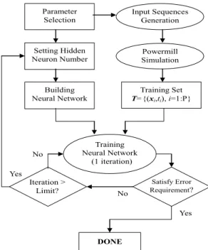
Since neural networks have been used for many years in other areas, determination of those parameters in neural networks is still mostly done by heuristic approaches. In typical experience, these parameter determinations are application-oriented problems. Different applications might have different suitable parameters of modeling construction. Therefore, the primary goal in this paper is trying to build a systematic procedure to build the power models using neural networks. The best parameters in the neural net-works might still be different from circuit to circuit.The overall construction procedure of the proposed neural power model is illus-trated in Fig. 4. This procedure consists of three major steps: building a neural network, generating training sets, and training the neural network. In order to make good decisions at each step, we will use several simple experiments to explain the decision strategies in the following discussions.
Because there are a lot of good training methods for neural networks, we will di-rectly use them and focus our discussions in the first two phases in the following sections. The only two things that have to be decided are the target error and the maximum
Parameter Selection Input Sequences Generation Powermill Simulation Training Set T={(xi,ti), i=1:P} Building Neural Network Training Neural Network (1 iteration) Satisfy Error Requirement? DONE Yes Iteration > Limit? No No Yes Setting Hidden Neuron Number
Fig. 4. The workflow of building a neural power model.
number of iterations in the training process. Because our target is to use the neural power model to estimate the average power of a test sequence, we decide to use the mean square error (MSE) as the validation error function. During the training phase, we will hold the temporal weight matrix after each iteration and estimate the validation error according to this weight matrix. If the validation error is smaller than 0.0036, which can roughly im-ply that the estimation error using the validation set is near 6%, we will stop the training process. Otherwise, we will train the neural network again using the same training set. According to our experiences, the validation errors are often saturated after 15 training iterations for those benchmark circuits. Therefore, we set the upper bound of training iterations as 15. If the stop criterion is still not satisfied after 15 iterations, we will add more hidden neurons and train the new neural network again using the same training set.
3.1 Building Neural Network
As described in section 2, we decide to use the 3-layer fully connected feedforward neural network structure and the Levenberg-Marquardt training algorithm with the mean square error function in our power model. In the first step, we have to decide the input data type of this neural network, the number of hidden neurons and the transfer function of internal neurons. In typical experiences, the best decisions might be different in dif-ferent cases, which are hard to be theoretically analyzed. Therefore, we will use a simple experiment on the circuit C1355, which is arbitrarily chosen in ISCAS’85 benchmark circuits, to explain our decisions for those parameters. Because it is not feasible to show all detailed analysis for each circuit, we will try to verify the feasibility of our approach with complete benchmark set in section 4 by using the metrics defined in section 2.3.
3.1.1 Input data type and transfer function
In this work, the input data type of neural networks and the transfer function of in-ternal neurons are decided together because the most suitable transfer function depends on the behavior between the input data and the output values of the training set. If the relationship between input data and output values has non-linear characteristics, the ac-curacy of the trained neural networks would be lost when using a linear transfer function for internal neurons because it is similar to use a piece-wise linear curve to fit a non- lin-ear curve as illustrated in Fig. 1.
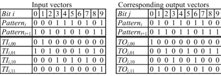
Since we are building a high-level power model, the input data of this neural power model can only use primary input and output information of circuits. The most straight-forward idea is to use the complete 4 states of bit transitions (0 → 0, 0 → 1, 1 → 0, 1 → 1) at the input and output pins of circuits as the input data of the neural networks because the effects of both state-dependent leakage power and transition-dependent switching power can be considered. If we use such bit-level transition data (bit-level statistics) to be the input data of our neural power model, the number of neurons in the input layer will be fixed as 4 × (n + m) for a circuit with n inputs and m outputs, which are TIi,00, TIi,01,
TIi,10, TIi,11, TOj,00, TOj,01, TOj,10 and TOj,11. Here, TIi,xy = 1 represents that the ith input pin
changes from logic state x to y and TOj,xy = 1 represents that jth output bit changes from
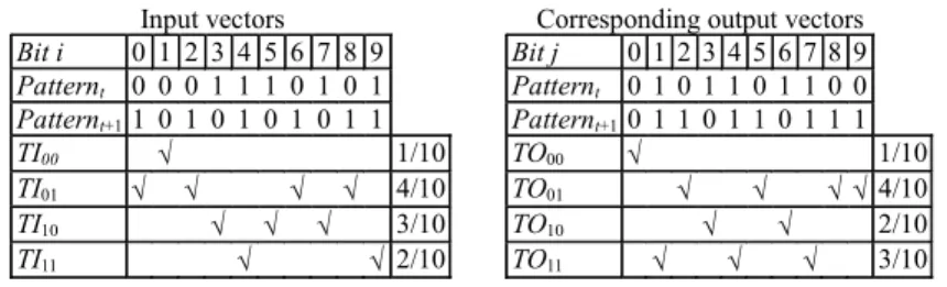
logic state x to y in a pattern pair. Instead of using bit-level statistics, we could use the word-level statistics as the input data of our neural power model. If we consider the input statistics and the output statistics separately, the number of neurons in the input layer will be fixed as 8, which are TI00, TI01, TI10, TI11, TO00, TO01, TO10 and TO11. Here, TIxy
repre-sents the ratio of input signals change from logic state x to y in a input pattern pair and TOxy represents the ratio of output signals change from logic state x to y in a output
pat-tern pair. For example, given a circuit with 10 inputs and 10 outputs, we assume that its corresponding output signals will change from 0101101100 to 0110110111 when the input signals change from 0001110101 to 1010101011. For this pattern pair, both the bit-level and word-level statistics are shown in the 4th to 7th rows in Figs. 5 (a) and (c) respectively. According to the definitions, their input data will be formed as shown in Figs. 5 (b) and (d). Input vectors Bit i 0 1 2 3 4 5 6 7 8 9 Patternt 0 0 0 1 1 1 0 1 0 1 Patternt+1 1 0 1 0 1 0 1 0 1 1 TIi,00 0 1 0 0 0 0 0 0 0 0 TIi,01 1 0 1 0 0 0 1 0 1 0 TIi,10 0 0 0 1 0 1 0 1 0 0 TIi,11 0 0 0 0 1 0 0 0 0 1
Corresponding output vectors Bit j 0 1 2 3 4 5 6 7 8 9 Patternt 0 1 0 1 1 0 1 1 0 0 Patternt+10 1 1 0 1 1 0 1 1 1 TOj,00 1 0 0 0 0 0 0 0 0 0 TOj,01 0 0 1 0 0 1 0 0 1 1 TOj,10 0 0 0 1 0 0 1 0 0 0 TOj,11 0 1 0 0 1 0 0 1 0 0 Fig. 5. (a) An example of the bit-level statistics characterization.
total length = 40 bit-level statistics
Input vector part Corresponding output vector part TI0,00 TI0,01 . . . TI9,10 TI9,11 TO0,00 TI0,01 . . . TI9,10 TI9,11
0 1 … 0 1 1 0 … 0 0
Input vectors Bit i 0 1 2 3 4 5 6 7 8 9 Patternt 0 0 0 1 1 1 0 1 0 1 Patternt+1 1 0 1 0 1 0 1 0 1 1 TI00 √ 1/10 TI01 √ √ √ √ 4/10 TI10 √ √ √ 3/10 TI11 √ √ 2/10
Corresponding output vectors Bit j 0 1 2 3 4 5 6 7 8 9 Patternt 0 1 0 1 1 0 1 1 0 0 Patternt+10 1 1 0 1 1 0 1 1 1 TO00 √ 1/10 TO01 √ √ √ √ 4/10 TO10 √ √ 2/10 TO11 √ √ √ 3/10
Fig. 5. (c) An example of the word-level statistics characterization.
total length = 8 (fixed) word-level statistics
Input vector part Corresponding output vector part TI00 TI01 TI10 TI11 TO00 TO01 TO10 TO11 0.1 0.4 0.3 0.2 0.1 0.4 0.2 0.3
Fig. 5. (d) Input data format with word-level statistics.
If we use bit-level statistics to be the input data of our neural power model, the neu-ral network may recognize the individual contribution to the total power consumption from each input transition such that the estimation error of the power model is more pos-sible to be reduced. However, the size of this power model will increase very fast espe-cially for the circuits with large amount of I/O pins. Moreover, because the complexity of bit-level statistics is too high, it will become much harder to learn such complex rela-tionship between the bit-level statistics and the power consumptions for a neural network. If we use word-level statistics as the input data of neural power model, some individual characteristics of each possible input transition may be lost, especially for the control- dominated circuits with significantly different power modes. However, it is a common heuristic method used in many power models [5, 8, 12, 24] to reduce the modeling com-plexity with reasonable error loss. According to their experimental results, the induced errors are indeed in an acceptable range in most cases.
When we are selecting the transfer function, we also have to consider the output format of our neural power model. The output of our neural power model is expected to represent the estimated power consumption of pattern pairs. Because the values of power consumptions often continuously distribute on a wide range, those transfer functions that use discrete values, such as the unit-step or the sign functions are not suitable. In our observations, the three commonly used functions, logarithmic sigmoid (logsig), hyper-bolic tangent sigmoid (tansig) and linear (linear) functions, are more suitable for our application, which are defined in Eqs. (10), (11) and (12) respectively. However, it should be noted that the values of power consumption have to be normalized between 0 to 1 in both the training set and the test set if logarithmic sigmoid and hyperbolic tangent sigmoid functions are used in the output neuron. In order to save the normalization effort, we use the linear function as the transfer function of the output neuron. In the following discussions, we will focus on the comparison between those three transfer functions for hidden neurons.
logsig transfer function: ( ) 1 1 s
f s
e−
=
tansig transfer function: ( ) 2 2 1 1 s f s e− = − + (11)
linear transfer function: f(s) = s (12)
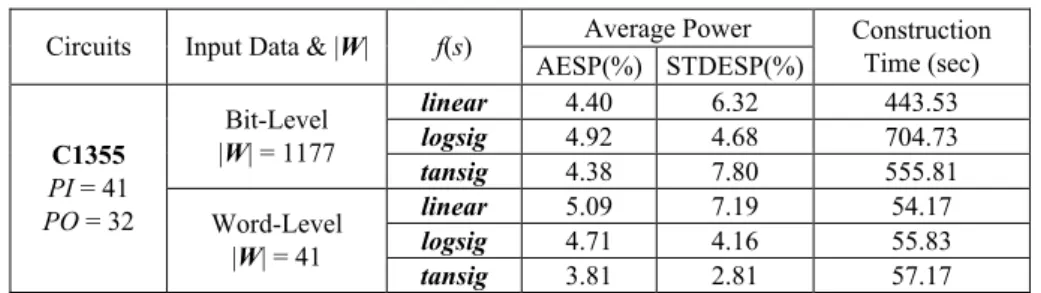
In order to help us making better decisions, we perform an experiment to compare the accuracy and performance of 6 combinations between 2 input data types (bit-level and word-level statistics of the input and output pattern pairs) and 3 transfer functions (logsig, tansig, linear). Because this experiment is only used for evaluating the input data types and suitable transfer functions, many parameters in the neural network are arbitrar-ily chosen and fixed in this experiment. All the training process will be stopped after 15 iterations instead of using the validation error checking as the stop criterion. The number of hidden neurons is fixed as 4. The training set includes 20 sequences, which are uni-formly distributed over the population of the average signal probability (Pin) and the
av-erage signal transition density (Din) and each sequence includes 1,000 random input
pat-tern pairs with the chosen PD combination. The comparison using AESP and STDESP for those test cases on C1355 is shown in Table 1.
Table 1. Comparison of input data types vs. transfer functions.
Average Power Circuits Input Data & |W| f(s)
AESP(%) STDESP(%) Construction Time (sec) linear 4.40 6.32 443.53 logsig 4.92 4.68 704.73 Bit-Level |W| = 1177 tansig 4.38 7.80 555.81 linear 5.09 7.19 54.17 logsig 4.71 4.16 55.83 C1355 PI = 41 PO = 32 Word-Level |W| = 41 tansig 3.81 2.81 57.17 The neural power model using bit-level statistics has higher complexity than that of the neural power model using word-level statistics, which can be observed in the number of weight |W| and the constructing time. However, as shown in the experimental results, the neural power model using bit-level statistics does not have many improvements in terms of AESP and STDESP. According to the analysis above, we select word-level sta-tistics as the input data of our neural power model. While checking the neural power model using word-level statistics, we can find that the neural power model using tansig function as the transfer function of hidden neurons provides better results on AESP and
STDESP. Therefore we select tansig function as the transfer function of internal hidden
neurons in this work.
3.1.2 Number of Hidden Neurons
Another issue to be decided is the number of hidden neurons required in the neural power model. Typically, the minimal number of hidden neurons depends on the com-plexity of the relationship between the input data and output values in the training set. However, according to the experience in neural network researches, there is no easy or
general way to determine the optimal solution for the number of hidden neurons to be used [23]. As mentioned in section 2, our strategy is initially using a neural network with a small number of hidden neurons and increasing the hidden neurons until the stop crite-rion has satisfied. In the following discussions, we will explain the reason of using this strategy through a simple experiment.
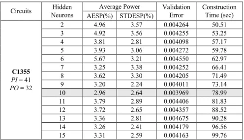
We first build a neural power model for C1355 and set the initial number of hidden neurons as 2. The training set is the same one as used in the experiment of section 3.1.1. The validation set includes 20 sequences with the same PD distribution as in the training set, but and the size of each sequence is increased to 3,000. In the following experiment, we increase the number of hidden neurons from 2 to 15 and test the accuracy of the neu-ral networks after 15 training iterations using the same test set as used in the experiment of section 3.1.1. The experimental results about the effects of number of hidden neurons are shown in Table 2.
Table 2. The effects of number of hidden neurons.
Average Power Circuits Neurons Hidden
AESP(%) STDESP(%) Validation Error Construction Time (sec) 2 4.96 3.57 0.004264 50.51 3 4.92 3.56 0.004255 53.25 4 3.81 2.81 0.004098 57.17 5 3.93 3.06 0.004272 59.78 6 5.67 3.21 0.004550 62.97 7 3.25 3.38 0.004252 66.41 8 3.62 3.30 0.004205 71.49 9 3.20 2.24 0.004011 73.14 10 2.96 2.64 0.003969 78.99 11 3.79 2.89 0.004406 81.83 12 3.72 2.65 0.004357 88.52 13 3.36 2.81 0.004675 90.28 14 3.26 2.41 0.004179 96.56 C1355 PI = 41 PO = 32 15 3.31 2.59 0.004163 99.76
According to the results in Table 2, increasing the number of hidden neurons does improve both AESP and STDESP when the number is small. However, when the number of hidden neurons is larger than 10, we could find that the validation error, AESP, and
STDESP may become worse due to the over fitting problem mentioned in section 2.2.
Therefore, for this case, the best choice is to set the number of hidden neurons as 10.
3.2 Design of Training Sets
Typically, a power model is expected to be used for different test sets with various input distributions. In order to achieve this target, the neural power model should be trained over a wide range in the input space such that it can learn enough experiences.
Therefore, we will randomly decide the Pin and Din while generating each test sequence.
is a relationship between Pin and Din as shown in Eq. (13), whose detailed proof can be
found in [8]. Therefore, while generating those training sets over a wide range of Pin and
Din distribution, we can use only the PD combinations that satisfy Eq. (13) such that
neu-ral networks could learn the correct characteristics between the input signal statistics and the power consumption of circuits.
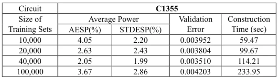
1 2 2 in in in D D P ≤ ≤ − (13) The size of a training set is also an important issue while training the neural power model. According to the related study [22], it suggested to determine the size of training set according to Eq. (14), in which P is the number of samples, |W| is the number of weights to be adjusted and a is the expected accuracy. In this work, our target is set as a ≥ 95%. According to this error requirement, we suggest to generate the training set with size P >> 20 |W|. A larger training set is supposed to produce a more accurate neural power model. However, the characterization time of this power model is also increased. In the following experiment, we will show the observation of the relationship between the size of training set and the modeling accuracy.
1 P a > − W (14) In this experiment, we use the best neural network structure for C1355 decided in section 3.1, which is a neural network that uses 10 hidden neurons and word-level statis-tics. As mentioned above, the samples of the training sets should be distributed over the space with a wide range of Pin and Din. Therefore, we generate 4 training sets consisting
of 20 sequences in each, which have the same uniformly distribution on the input space that satisfies the Pin and Din constrains in Eq. (13). However, the length of each sequence
is different, which are 500, 1,000, 2,000 and 5,000 pattern pairs respectively. In other words, the total sizes of the training sets are 10,000, 20,000, 40,000 and 100,000 respec-tively. The validation sets consist of 20 sequences that have the same distribution as those test sequences but their sequence lengths are multiplied by 3. Therefore, the sizes of validation sets are 30,000, 60,000, 120,000 and 300,000 respectively. The experimen-tal results of those 4 neural networks under different training conditions after 15 training iterations, which are evaluated using the same test set that consists of 20 sequences with 3,000 pattern pairs are shown in Table 3.
Table 3. The effects of the size of training set.
Circuit C1355
Average Power Size of
Training Sets AESP(%) STDESP(%)
Validation Error Construction Time (sec) 10,000 4.05 2.20 0.003952 59.47 20,000 2.63 2.43 0.003804 99.67 40,000 2.05 1.99 0.003510 114.21 100,000 3.67 2.86 0.004203 233.95
The experimental results show that the size of training set will not affect the accu-racy too much on accuaccu-racy if the training set is large enough. According to this observa-tion, we generate 20 sequences with 3,000 pattern pairs in each sequence to be the train-ing set of our neural power model in the followtrain-ing experiments to make a trade off be-tween the size of test sequences and accuracy. Of course, those 20 sequences will have a distribution that covers a wide range of the input space.
4. EXPERIMENTAL RESULTS
In this section, we will demonstrate the accuracy and efficiency of our power model with ISCAS’85 benchmark circuits and one real design, a combinational divider with 32-bit dividend/quotient and 12-bit divisor/remainder. All circuits in our experiments were synthesized by using 0.35μm cell library. The accuracy will also be compared with traditional 3D-LUT power modeling methodology, which uses Pin, Din and average
out-put signal transition density (Dout) as its three dimensions, and the interval size of each
dimension is set to 0.1. Our neural power models including the training algorithms were all constructed on MATLAB by using an Intel Pentium III 1GHz mobile CPU and 384M RAM.
In the model construction phase, the input training sequences are generated over a wide range of input distribution as described in section 3.2. The real power of those input sequences is simulated by a transistor-level simulator, PowerMill such that the measured power consumptions can include switching power and leakage power and can be charac-terized in the power model. In order to show the power models can be used for various input distribution, we test those models by using 200 test sequences with 3,000 pattern pairs. Each sequence has different Pin and Din that are randomly selected over a wide
range that satisfies the condition in Eq. (13). After simulation, the estimated average power consumption with this power model is also compared to the simulation results from PowerMill.
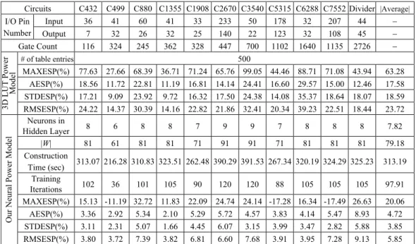
All the test circuits will be tested using the two power estimation approaches with the same information: traditional 3D-LUT power model and our neural power model. The same training and test sequences will be used for both approaches to make a fair comparison. The performances of both power models are summarized in Table 4. The construction time of neural power models includes the data pre-loading time of training and validation sets, the establishing time of neural network and the elapsed time of net-work training process. The simulation time of transistor-level simulation is not included.
According to Table 4, the average values of AESP and STDESP are 17.58% and 18.59% respectively while we use the traditional 3D-LUT power models. The conver-gences of this approach are quite poor that can be observed from the large values of STDESP. It implies that using the LUT-based power model may have large errors in some cases. Compared to the traditional 3D-LUT power model, we only have 4.72% error for all cases on average, and the largest AESP is only 8.93% for the 32-bit divider. The improvement of our neural power model can be shown in the STDESP. The largest
STDESP is only 5.88% for the 32-bit divider using our approach, which shows a good
agreement with real powers. The combined scatter plots of all ISCAS’85 circuits by us-ing our approach and the 3D-LUT approach are shown in Figs. 6 and 7 respectively.
Table 4. The comparison between traditional 3D LUT power model and our neural power model.
Circuits C432 C499 C880 C1355 C1908 C2670 C3540 C5315 C6288 C7552 Divider |Average|
Input 36 41 60 41 33 233 50 178 32 207 44 − I/O Pin Number Output 7 32 26 32 25 140 22 123 32 108 45 − Gate Count 116 324 245 362 328 447 700 1102 1640 1135 2726 − # of table entries 500 MAXESP(%) 77.63 27.66 68.39 36.71 71.24 65.76 99.05 44.46 88.71 71.08 43.94 63.28 AESP(%) 18.56 11.72 22.81 11.19 16.81 14.14 24.41 16.60 29.57 15.00 12.46 17.58 STDESP(%) 17.21 9.09 23.92 9.72 16.32 17.50 24.38 14.08 35.37 18.64 18.07 18.59 3D LUT Power Model RMSESP(%) 24.22 14.37 30.39 14.16 22.82 21.86 32.41 20.34 39.23 22.51 18.44 23.72 Neurons in Hidden Layer 8 6 8 8 7 9 9 7 8 8 8 7.82 |W| 81 61 81 81 71 91 91 71 81 81 81 79.18 Construction Time (sec) 313.07 216.28 310.83 323.51 262.48 390.29 391.53 267.34 320.19 324.29 325.23 313.19 Training Iterations 102 36 101 105 90 120 120 88 105 105 105 97.91 MAXESP(%) 15.13 -11.19 32.72 11.83 22.09 24.74 24.14 -17.28 16.34 -17.49 26.63 20.06 AESP(%) 3.36 2.92 5.34 2.10 5.29 5.72 4.57 3.83 4.14 5.47 8.93 4.72 STDESP(%) 3.11 2.31 5.07 1.66 4.45 6.07 3.15 3.99 3.47 2.82 5.88 3.85
Our Neural Power Model
RMSESP(%) 3.80 3.72 7.39 3.82 6.81 6.60 7.68 3.91 3.95 7.28 9.13 5.85
Fig. 6. Scatter plot of neural power model estimation versus PowerMill simulation in ISCAS’85 benchmarks.
In order to examine all circuits on the same plot, the power consumptions of all circuits are normalized with the circuit size and operating frequency. Comparing the two plots, we can see that our approach can really provide better trend of estimation accuracy.
The storage requirements are also much less in our approach. According to the re-sults shown in Table 4, the maximum number of hidden neurons is 9 in our experiments.
Fig. 7. Scatter plot of 3D-LUT estimation versus PowerMill simulation in ISCAS’85 benchmarks.
It means that we only use up to 9 hidden neurons structure with 91 elements in the weight matrix |W| to record the power characteristics, which is quite small compared to the lookup tables, which require 500 (= 10 × 10 × 10/2) numbers to record the tables. These experimental results have also shown that the complexity of our neural power model has almost no relationship with circuit size and number of inputs and outputs. Even for large circuits such as the 32-bit divider, the complexity of its power model is still the same as the complexity of smaller circuits such as C432. Besides, the construc-tion of neural power model is rapid that can be observed from the short construcconstruc-tion time and the total training iterations of each neural power model in Table 4. Therefore, using such a power model can be very efficient even for complex circuits and also has high accuracy.
Another important information not shown in Table 4 is the estimation time while using our power model. Actually, the estimation time of our neural power model is dominated by the functional simulation time with a logic simulator, which simulates the circuits with specific input vectors to obtain the corresponding output vectors. If we as-sume that the corresponding output values under specific input sequences are also pro-vided by users, the estimation time of our neural power model is always less than one second for all ISCAS’85 circuits. Therefore, the estimation time is not shown in Table 4 because it is almost equal to the logic simulation time, which is quite small compared with low-level power estimation methods such as PowerMill.
In order to demonstrate that the neural power model can handle specific functional patterns in practical use, we also test the practical design, the 32-bit divider design, with user-given functional patterns. The functional sequence consists of 1,000 pattern-pairs only. However, the average estimation error is only 5.98% compared to the PowerMill results.
6. CONCLUSIONS
uses neural networks to learn the power characteristics during simulation including both leakage power and switching power. Unlike the power characterization process in tradi-tional approaches, our characterization process is very simple and straightforward. The complexity of our neural power model is also less than traditional 3D LUT power model which is almost no relationship with circuit size and the number of inputs and outputs. More importantly, using the neural power model for power estimation does not require any detailed circuit information of the circuits, which is very suitable for IP protection. In this paper, we have tested our neural power model on all ISCAS’85 benchmark circuits and one real design. The experimental results demonstrate that our neural power model can accurately estimate the power consumption of combinational circuit for different test sequences with wide range of input distributions.
REFERENCES
1. S. Y. Huang, K. C. Chen, et al., “Compact vector generation for accurate power simulation,” in Proceedings of the ACM/IEEE Design Automation Conference, 1996, pp. 161-164.
2. R. Marculescu, D. Marculescu, and M. Pedram, “Sequence compaction for power estimation: theory and practice,” IEEE Transactions on Computer-Aided Design of
Integrated Circuits and Systems, Vol. 18, 1999, pp. 973-993.
3. A. Pina and C. L. Liu, “Power invariant vector sequence compaction,” in
Proceed-ings of the ACM/IEEE International Conference on Computer-Aided Design, 1998,
pp. 473-476.
4. F. N. Najm, “A survey of power estimation techniques in VLSI circuits,” IEEE
Transactions on VLSI Systems, Vol. 2, 1994, pp. 446-455.
5. P. Landman, “High-level power estimation,” in Proceedings of the International
Symposium on Low Power Electronics and Design, 1996, pp. 29-35.
6. M. Nemani and F. Najm, “Towards a high-level power estimation capability,” IEEE
Transactions on Computer-Aided Design, Vol. 15, 1996, pp. 588-598.
7. D. Marculescu, R. Marculescu, and M. Pedram, “Information theoretic measures for power analysis,” IEEE Transactions on Computer-Aided Design, Vol. 15, 1996, pp. 599-610.
8. S. Gupta and F. N. Najm, “Power modeling for high-level power estimation,” IEEE
Transactions on VLSI Systems, 2000, pp. 18-29.
9. R. Corgnati, E. Macii, and M. Poncino, “Clustered table-based macromodels for RTL power estimation,” in Proceedings of the 9th Great Lakes Symposium on VLSI, 1999, pp. 354-357.
10. A. Bogliolo, R. Corgnati, E. Macii, and M. Poncino, “Parameterized RTL power models for soft macros,” IEEE Transactions on VLSI Systems, Vol. 9, 2001, pp. 880-887.
11. C. Y. Hsu, C. N. J. Liu, and J. Y. Jou, “An efficient IP-level power model for com-plex digital circuits,” in Proceedings of Asia South Pacific Design Automation
Con-ference, 2003, pp. 610-613.
12. S. Gupta and F. N. Najm, “Analytical models for RTL power estimation of combina-tional and sequential circuits,” IEEE Transactions on Computer-Aided Design, Vol. 19, 2000, pp. 808-814.
13. Q. Wu, Q. Qiu, M. Pedram, and C. S. Ding, “Cycle-accurate macro-models for RT-level power analysis,” IEEE Transactions on VLSI Systems, Vol. 6, 1998, pp. 520-528.
14. S. Gupta and F. N. Najm, “Energy-per-cycle estimation at RTL,” in Proceedings of
the ACM/IEEE International Symposium on Low Power Design, 1999, pp. 121-126.
15. E. Macii and M. Poncino, “Estimating power consumption of CMOS circuits mod-eled as symbolic neural networks,” IEE Proceedings on Computers and Digital
Techniques, 1996, pp. 331-336.
16. J. H. Hopfield, “Artificial neural networks,” IEEE Circuits and Devices Magazine, 1988, pp. 3-10.
17. R. I. Bahar, E. A. Frohm, C. M. Gaona, G. D. Hachtel, E. Macii, A. Pardo, and F. Somenzi, “Algebraic decision diagrams and their applications,” in Proceedings of
the IEEE/ACM International Conference on Computer-Aided Design, 1993, pp.
188-191.
18. L. Cao, “Circuit power estimation using pattern recognition techniques,” in
Pro-ceedings of the IEEE/ACM International Conference on Computer-Aided Design,
2002, pp. 412-417.
19. T. L. Fine, Feedforward Neural Network Methodology, Springer, New York, 1999. 20. K. Levenberg, “A method for the solution of certain problem in least square,”
Quar-terly of Applied Mathematics, Vol. 11, 1944, pp. 164-168.
21. D. W. Marquardt, “An algorithm for least squares estimation of non-linear parame-ters,” Journal of the Society for Industrial and Applied Mathematics, Vol. 11, 1963, pp. 431-441.
22. E. B. Baum and D. Haussler, “What size net gives valid generalization?” Neural
Computation, Vol. 1, 1989, pp. 151-160.
23. K. Mehrotra, C. K. Mohan, and S. Ranka, Elements of Artificial Neural Networks, MIT Press, Cambridge, Massachusetts, 1997.
24. G. Jochens, L. Kruse, E. Schmidt, and W. Nebel, “A new parameterizable power macro-model for datapath components,” in Proceedings of the European Design and
Test Conference, Date, 1999, pp. 29-36.
Chih-Yang Hsu (許智揚) is a Ph.D. candidate in the
De-partment of Electronics Engineering at the National Chiao Tung University, Taiwan, R.O.C. His primary research interest is power estimation of designs in each design level. He holds a B.S. in Computer and Information Science from the National Chiao Tung University.
Wen-Tsan Hsieh (薛文燦) received the M.S. degree in
Electronics Engineering from National Central University, Tai-wan, R.O.C. He is currently working toward the Ph.D. degree in Electrical Engineering at National Central University. His pri-mary research interest is high-level power estimation.
Chien-Nan Jimmy Liu (劉建男) received the B.S. and
Ph.D. degrees in Electronics Engineering from National Chiao Tung University, Taiwan, R.O.C. He is currently an assistant professor in the Department of Electrical Engineering at National Central University. His research interests include functional veri-fication for HDL designs, veriveri-fication of system-level integration, and high-level power modeling. He is a member of Phi Tau Phi.
Jing-Yang Jou (周景揚) received the B.S. degree in
Elec-trical Engineering from National Taiwan University, Taiwan, R.O.C., and the M.S. and Ph.D. degrees in Computer Science from the University of Illinois at Urbana-Champaign, in 1979, 1983, and 1985, respectively. He is currently the Director Gen-eral of National Chip Implementation Center, National Applied Research Laboratories in Taiwan. He is a full Professor and was Chairman of Electronics Engineering Department from 2000 to 2003 at National Chiao Tung University, Hsinchu, Taiwan. Be-fore joining Chiao Tung University, he was with GTE Laborato-ries and AT&T Bell LaboratoLaborato-ries. His research interests include logic and physical syn-thesis, design verification, CAD for low power and Network on Chips. He has published more than 100 technical papers. Dr. Jou is a Fellow of IEEE. He is a member of Tau Beta Pi, and the recipient of the distinguished paper award of the IEEE International Confer-ence on Computer-Aided Design, 1990. He served as the Technical Program Chair of the Asia-Pacific Conference on Hardware Description Languages (APCHDL’97).