建立連續性滿足點的Phase II/III調適設計來評估來藥物之效能性

全文

(1)國立交通大學統計學研究所碩士論文. 建立連續性滿足點的 Phase II/III 調適設計來評估藥物之效能性 A Phase II/III Adaptive Design for Evaluation of Drugs Efficacy Based on Continuous Endpoints. 研究生：黃翁賢指導教授：蕭金福. 教授. 中華民國九十七年六月.

(2) 建立連續性滿足點的 Phase II/III 調適設計來評估藥物之效能性 A Phase II/III Adaptive Design for Evaluation of Drugs Efficacy Based on Continuous Endpoints. 研究生：黃翁賢. Student：Wong-Shian Huang. 指導教授：蕭金福. Advisor：Chin-Fu Hsiao. 國立交通大學統計學研究所碩士論文. A Thesis Submitted to Institute of Statistics College of Science National Chiao Tung University in partial Fulfillment of the Requirements for the Degree of Master in Statistics June 2008 Hsinchu, Taiwan, Republic of China. 中華民國九十七年六月.

(3) 建立連續性滿足點的 Phase II/III 調適設計來評估藥物之效能性研究生 : 黃翁賢. 指導教授: 蕭金福博士. 國立交通大學統計學研究所. 中文摘要. 醫藥發展是一具風險的、複雜的、昂貴和費時的產業。大部分的發展時間皆耗費於臨床實驗的執行。儘管目前仍存在大量的候選藥物以及蓬勃的臨床研究發展，但成功率仍然令人非常失望。因此，急需發展有效率且節省成本的新方法。一般而言，以連續性滿足點的 phase II 試驗，主要目的為檢驗藥物的有效性、以及決定劑量範圍與劑量反映的相關性。因而從 phase II 試驗，便有一種或多種不同劑量之藥物，可能會同時進入 phase III 的試驗。目前以連續性滿足點的 phase II 試驗，大部份均利用標準平行藥物反映與安慰劑群組的設計，經由不同劑量與安慰劑兩兩間之比較，藉由 p-value 的調整，來決定劑量範圍與劑量反映。因此在 phase II 階段，便可能需要數以百計甚致於數以千計的病人，而且花費的時間也可能需要兩到三年。儘管如此，能夠進到 phase III 的試驗，成功的機率也是非常的小。此研究中，我們針對連續性滿足點的臨床試驗，發展一個 phase II/III 的試驗設計來評估候選藥物的效能性。在 phase II 試驗，包含多種不同劑量之群組與安慰劑群組。在此階段，如果藥物劑量有效性與劑量所對應的直線斜率大於預先假設值時，亦即此藥物各劑量的效能均比安慰劑群組為佳，如此我們便可選擇ㄧ種藥效最好的劑量與安慰劑群組進入 phase III 試驗，否則便停止此藥物的試驗。而且，所有進到 phase III 試驗群組之 phase II 的病人均可進到 phase III 試驗，如此便可減少試驗所需的樣本數，因而縮短試驗所需的時間。於控制型一錯誤與統計檢定力的條件下，我們可計算各個階段所需的樣本數以及各個階段之檢定統計量的臨界值。. i.

(4) A Phase II/III Adaptive Design for Evaluation of Drugs Efficacy Based on Continuous Endpoints Student: Wong-Shian Huang. Advisor: Dr. Chin-Fu Hsiao. Institute of Statistics National Chiao Tung Unveristy. Abstract. Pharmaceutical development is a risky, complex, costly and time-consuming endeavor. More than half of development duration is spent in clinical trials. Despite of a large amount of the potential candidates available and the lengthy process of clinical development, success rate is disappointed. Accordingly, there is an urgent need of new strategies and methodology for efficient and cost-effective designs towards the conduct of clinical trials in a rapid and reliable manner to minimize the total sample size and hence to shorten the duration of the trials. In this paper, a phase II/III adaptive design based on continuous efficacy endpoints is proposed. For the phase II part, the design is a randomized parallel group with several doses and a concurrent placebo group. Suppose that the dose-response relationship can be described by the simple linear regression. If the slope is greater than a pre-specified positive number, we will continue the accrual for the best dose group as well as the placebo group for the phase III trial. After the recruitment of the patients in the phase III trial is completed, we then perform the final analysis with the cumulative data of patients from both phases for both groups. We can also determine the sample size required for each group in each phase.. KEY WORDS: Adaptive design, Clinical trial, Phase II/III design.. ii.

(5) 誌謝這篇論文的完成，最要感謝指導教授，蕭金福老師不倦不悔的指導與批閱。兩年前，剛進交大統研時，還是個小碩士生，對研究還未接觸過，和蕭老師一起做研究後，帶領我進入學術界的殿堂，對尚未解決的問題努力著。如今已完成論文，希望為社會進一份貢獻，期勉讓更多領域銜接與應用。同時也感謝口試委員劉仁沛教授、鄒小蕙博士、洪慧念教授提供諸多建議，使得這本論文更臻完善。研究所期間，感謝所上教授們提供的授課環境與教學內容，增進統計更專業的知識與經驗以及同學們積極向學的精神。生活上也很感謝家人給予的支持與鼓勵。謹以此論文獻給我的家人、師長、同學及朋友，以表達心中最誠摯的感激。. 黃翁賢謹誌于國立交通大學統計學研究所中華民國九十七年六月. iii.

(6) Content 中文摘要........................................................................................................................ I ABSTRACT.................................................................................................................II 誌謝............................................................................................................................. III CONTENT................................................................................................................. IV 1. INTRODUCTION....................................................................................................1 2. A PHASE II/III ADAPTIVE DESIGN...................................................................4 3. RESULTS..................................................................................................................9 4. DISCUSSIONS.......................................................................................................12 REFERENCES...........................................................................................................14 LIST OF TABLES......................................................................................................15 LIST OF FIGURES ...................................................................................................17. iv.

(7) 1. Introduction Pharmaceutical development is a risky, complex, costly and time-consuming endeavor. Developing a drug from screening of candidates to regulatory approval for commercial marketing usually takes more than 12 years with an average cost between 800 millions and one billion US dollars. Mostly, 70% of the cost for pharmaceutical development is wasted upon the drug that does not even make it to market. In addition, more than half of development duration is spent in clinical trials. Despite of a better understanding of disease etiology and advance in medical technology, only one out of 10,000 candidates screened in the laboratory will survive to the market launch. More than 60% of the potential candidates that enter into the clinical development fail. Furthermore, the success rate of the phase III stage of the clinical development has fallen by 30% (The Economist (2002)). The possible reasons for this failure include different patient populations for the phase II and III trials, surrogate endpoints used by the phase II trials, different experimental conditions due to medical advances.. As a result, the total duration of drug development is increased. Currently, the pharmaceutical industry as a whole encounters a tremendous challenge of search for new strategy and methodology that can be applied to the conduct of clinical development to improve the overall success rate and to cut down the lengthy period of drug development. Consequently, there is an urgent need for efficient and cost-effective designs towards the conduct of clinical trials in a rapid and reliable manner to minimize the total sample size and hence to shorten the duration of the trials. For the cytotoxic agents for cancer treatment, procedures of selecting the potential regimens not based on statistical significance for the pairwise comparisons have been proposed based on the binary and survival endpoints (Simon et al. (1985); Liu et al. (1992)). On the other hand, a combined phase II/III program was also suggested for cancer drugs (Schaid et al. (1990); Scher and Heller (2002)). However, the above-mentioned approach of the randomized phase II trials and phase II/III program has not been applied to the drugs other than the cancer cytotoxic agents.. If the primary efficacy endpoint for evaluation of a potential drug candidate for treatment of a certain disease is a continuous variable, Tsou et al. (2008) have. 1.

(8) proposed a two-stage screening design with no control group. The proposed two-stage screening designs minimize the expected sample size if the new candidate has low efficacy activity subject to the constraint upon the type I and type II error rates. In some cases, the objectives of phase II studies in the clinical development are to initially assess the efficacy, and to determine the dosing range and dose response relationship. Therefore one or several doses from the phase II studies are selected to enter into the phase III studies in more broad and heterogeneous patient population for further confirmation of the efficacy and safety observed in the phase II studies. The current approach of the phase II studies with continuous endpoints starts with the titration design for preliminary evaluation of efficacy and then followed by the standard randomized parallel dose-response design with a concurrent placebo group for determination of dosing range and dose response (Chow and Liu (2004)). Pairwise comparisons between dose and placebo are usually performed with adjustment of p-values to determine the dosing range and dose response. Several hundred to a thousand patients are usually required for the phase II trials with an average between two to three years to complete. Hence, there is an urgent need of new strategies and methodology for efficient and cost-effective designs to shorten the duration of the trials or improve the success rate.. In recent years, the use of adaptive design methods in clinical research and development based on accrued data has become very popular due to its flexibility and efficiency. Therefore, in this paper, we will apply this concept to develop a phase II/III adaptive design for evaluation of drugs efficacy based on continuous endpoints. The purposes of our phase II/III trials are: (1) the same targeted patient population is assessed in the same phase II/III trial with the same primary continuous endpoints, evaluation criteria, schedules, and the same experimental conditions using the same protocol. (2) To describe a dose-response relationship among different doses. (3) To identify one dose with efficacy exceeding the pre-specified level for phase III part of the trial. Therefore the design for the proposed phase II/III trial consists of phase II and phase III parts. The design for the phase III part is the traditional randomized parallel group either with a concurrent placebo group or with a concurrent standard treatment. In this paper, the design of phase II/III for evaluation of drugs efficacy based on continuous endpoints is described in Section 2. Some numerical results are. 2.

(9) given in Section 3. Discussion and final remarks are provided in Section 4.. 3.

(10) 2. A Phase II/III Adaptive Design For simplicity, we only focus on the trials for comparing a test product with several doses and a placebo control. For the phase II part, the design is a randomized parallel group with several doses, say d1 , d 2 ,..., d k , and a concurrent placebo group ( d 0 ). Let Yij be the observed continuous endpoint for patient j assigned to dose d i , i=0,…,k. We also assume that Yij follows a normal distribution with mean i and known variance  2 , i=0,1,…,k. The current approach to assessing the dose-response is based on the following hypothesis: H 0 : i   0  0 vs. H A :  i   0  , i=1,…, k.. (1). Multiple comparison procedure can be used to test the above hypothesis. Since the formal statistical hypothesis testing for pairwise comparison is performed, the required sample size can be quite large if the detected difference is even moderate. On the other hand, the above hypothesis does not directly address the dose-response relationship. Suppose that the dose-response relationship can be described by the simple linear regression as follows: E Yij     d i .. As a result, the hypothesis of interest for our proposed phase II part is H 0II :   c vs. H IIA :   c,. (2). for some pre-specified c>0. Because hypothesis (2) is to verify whether the slope is positive, the required sample size will be generally smaller than that for hypothesis (1). However, a positive slope can not identify the doses for phase III part. Suppose that a positive linear relationship is established by rejecting the null hypothesis (2) at a certain significance level. Therefore, we can select one or more doses for phase III stage. Here,  0 is the mean of the placebo group and is assumed to have the smallest efficacy response. Let. . be the required minimal clinically meaningful. improvement on efficacy for a dose to be selected for the phase III stage. In other words, i   0 must be greater than  in order to select d i for the phase III stage. Then the sample size can be determined to ensure that if some doses are superior to placebo by the pre-specified amount  , a dose will be selected with high probability,. 4.

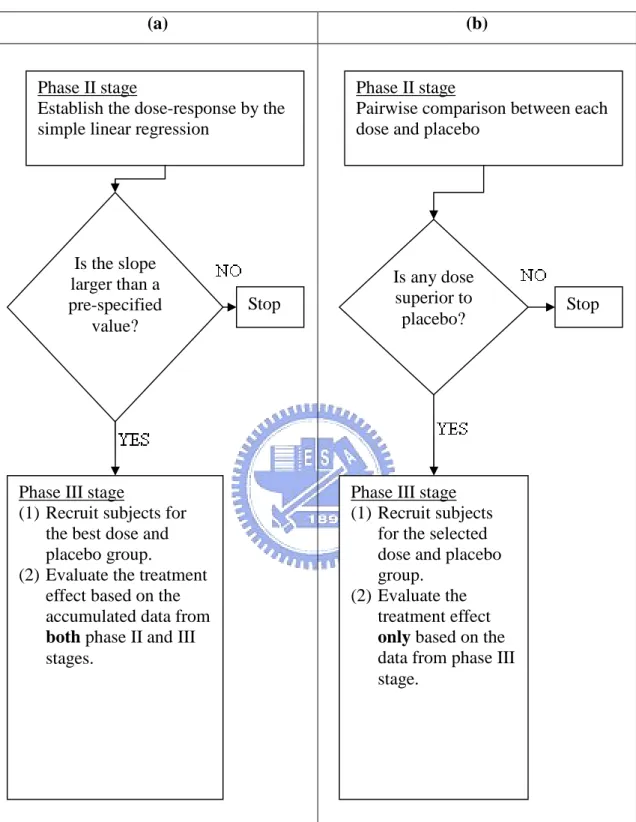
(11) say 0.8. Because no pairwise hypothesis testing with consideration of significance level and power is performed, the required sample size will be much smaller than the traditional phase II studies.. The schema of our proposed phase II/III adaptive design and the traditional approach is shown in Figure 1. Our approach for the phase II part is first to establish the dose-response relationship and then to select one dose based on the pre-specified minimal clinically meaningful improvement, and thus the success rate of the phase III studies may be improved. Since the sample size for our proposed phase II design is small, the phase II part can be completed in a much shorter duration. Therefore, our phase II/III design may be more efficient than the current paradigm with a better success rate.. Let n2 be the sample size per group for the phase II stage. The estimator of  is k. ˆ . n2.  (d i  0 j 1. i.  d )(Yij  Y ). 2. (d i  d ). ,. k. n i 0. 2. where k. d. d . i 0. i. k 1. ,. and n2. k. Y .  Y. ij. i  0 j 1. n 2 (k  1). .. We can derive. ˆ ~ N ( ,. 2 k.  n (d 2. i 0. . i. ), d). 2. . where N  , 2 is a normal prior with mean  and variance  2 . Assume that we will reject H0II if ˆ  C 2 . After rejecting H0II, suppose that the group with dose d r. 5.

(12) and the placebo group ( d 0 ) will be chosen into phase III. Let n3 be the sample size for phase III per group. Let  r and  0 be the respective means and let   i   0 . The hypothesis for phase III part is H 0III :   0 vs. H III A :   0.. The estimator of  is ˆ  Yr*  Y0* , where n2. n2  n3. j 1. j  n2 1.  Yrj . Yr  *. Y. rj. ,. n 2  n3. and n2. Y . Y. * 0. j 1. 0j. . n2  n3. Y. j  n2 1. 0j. n 2  n3. .. Consequently, we can derive 2 2 ˆ ~ N (  r   0 , ). n 2  n3 Assume that we will reject H0III if ˆ  C3 . Consequently, in the phase II/III design, the probability of rejecting the new drug with the true parameters  and  is a function of  , , n2 , n3 , C2 , C3 , and  and is given by.   , , n2 , n3 , C2 , C3 ,  . . .   P ˆ  C2    fˆ b P  C3  ˆ  C3 db, C2. (3). where P and P denote the probability measure with respect to  and  respectively, and fˆ () represents the probability density function of ˆ with respect to  . Let  denote the overall type I error rate. Consequently,  can be expressed as.   1 -  ( c,0, n2 , n3 , C2 , C3 ,  ) .  1  Pc (ˆ  C2 )   fˆ (b) P0 (C3  ˆ  C3 )db, C2. which can be written as  Pc (ˆ  C2 )   fˆ (b) P0 (C3  ˆ  C3 )db  1   . C2. (4). We need to determine how we want to spend the type I error rate,  , at each stage. Therefore we use a weighting factor  1 such that Pc (ˆ  C2 )   1 (1   ),. 6. (5).

(13) and. . . C2. fˆ (t ) P0 (C3  ˆ  C3 )dt  (1   1 )(1   ),. (6). where 0<  1 <1. As noted, larger  1 indicates that we spend fewer type I error rate for phase II stage. It is also obvious that the larger the  1 is, the larger the C2 is. Also when c is close to 0, if  1 is small, then the value of C2 satisfying (5) might be negative. A negative value of C2 indicates no treatment effect. Therefore, we suggest that  1 be greater than 0.6 if c=0.. Next let  be the type II error with a specified alternative hypothesis c and  . We can derive that.    ( c ,  , n2 , n3 , C 2 , C 3 ,  )   Pc ' (ˆ  C 2 )   fˆ (b) P ' (C 3  ˆ  C 3 )dt. C2. Again we need to determine how they want to spend the type II error probability at each stage. Consequently we introduce another weighting factor  2 such that Pc ' (ˆ  C 2 )   2  ,. (7). And. . . C2. fˆ (t ) P ' (C3  ˆ  C3 )dt  (1   2 )  ,. (8). where 0<  2 <1. As seen, the larger the  2 is, the smaller the n2 is. Considering    d r  d 0  under the linear trend, (3) can be re-expressed as.   , , n2 , n3 , C2 , C3 ,   n n    n2  P ˆ  C2    fˆ b P  2 3   C3  bd r  d 0   ˆ 3 C2 n2  n3   n3  . where. 7.  n2  n3  n2  C3  bd r  d 0  db, n3  n2  n3 .

(14) n2  n3. ˆ 3 . n2  n3. Y. j  n2 1. rj. . n3. Y. 0j. j  n2 1. .. n3. Under the specification of design parameters c, c, ,  1 ,  2 ,  , and  , the phase II/III adaptive design considered here is to determine n2 , n3 , C2 and C3 based on constraints of overall type I and II error rates given in (5), (6), (7), and (8).. Let n be the required sample size per dose level in traditional phase II trial for dose response to test the null hypothesis H 0 : i   0 against H A : i   0 , i=1,…, k at the phase II stage. Let  be the required minimal clinically meaningful improvement on efficacy for a dose to be selected for the phase III stage. Without considering multiple comparison, the sample size required for each dose group can be calculated by 2z  z  . 2. n .      . .. 2. (9). Alternatively, we can also apply the multiple comparison procedure. Let n B be the required sample size per dose level in traditional phase II trial using Bonferroni method for dose response. The sample size required for each dose group can be derived by 2z / k  z  . 2. n B .      . .. 2. (10). Let n be the required sample size per group in traditional phase III trial to test the null hypothesis H 0 :    r   0  0 against H A :    r   0  0 . Then the sample size required per group can be evaluated by 2z / 2  z  . 2. n .       . 8. 2. .. (11).

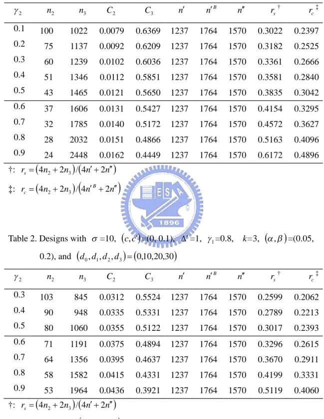
(15) 3. Results We give some examples for the purpose of illustration. Suppose the test drug has dose levels of 10, 20, and 30 respectively. Also assume that the placebo group has dose level of 0. Given  =10,  ,   = (0.05, 0.20), c =0, and c =0.1, Tables 1, 2, 3, and 4 illustrate the phase II/III designs for different combinations of design parameters with  1 =0.6 and 0.8, and  =1 and 2, respectively. For each  1 , we consider various combinations of values for  2 . The tabulated results include the required sample size ( n2 ) at the phase II stage, the required sample size ( n3 ) at the phase III stage, the critical value for the observed value of slope that would reject the test drug at the phase II stage ( C2 ), the critical value for the observed mean difference that would reject the test drug at the phase III stage ( C3 ), numbers of sample sizes required for the traditional phase II and phase III trials ( n , n  B , and n respectively), and the ratios of the total sample size for our phase II/III design vs. the total sample size for the traditional designs ( rs and rc ).. For instances, the first line in Table 1 considers the case of  =10, (c, c' ) = (0, 0.1), (,  ' ) = (0, 1), and  ,   = (0.05, 0.2). In this case, the phase II stage needs to recruit 100 patients for each group (i.e. 4×100=400 for total). When the study is completed at the phase II stage, if the observed value of slope ˆ does not exceed 0.0079, the trial is terminated after the phase II stage and considers the test drug is concluded as lack of efficacy. Oppositely, if the observed value of the estimator of slope ˆ is greater than 0.0079, the trial continues to phase III stage and assume that the dose level of 10 (i.e.  =1) is selected. We need to enroll additional 1022 patients for each group of the d 0 and d1 . After the recruitment of the patients at phase III stage is completed, if the overall observed absolute value of mean difference, ˆ , based on the cumulative data n2  n3 obtained at the end of the trial does not exceed 0.6369, we will reject the test drug. On the other hand, if the observed absolute value of ˆ is greater than 0.6369, we can conclude that the effect of test drug is different from that of the control group. In addition, the numbers of required sample sizes for. 9.

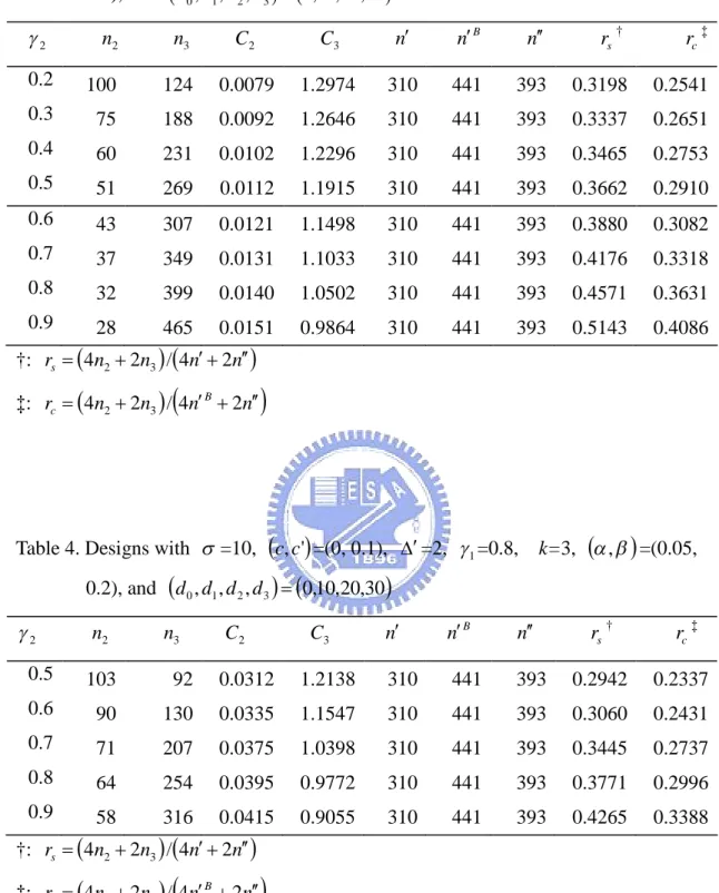
(16) the traditional phase II trial and phase III trial are 1237 (and 1764 for Bonferroni p-value adjustment) and 1570 per group respectively. In this case, the required total sample size for our phase II/III design can be reduced by around 33% and 76% respectively compared with two traditional approaches. From all tables, since all of values of rs and rc are less than 1, the required total sample size for our phase II/III design is possibly smaller than those required by the traditional methods.. From the tables, as  2 decreases, the required sample size per group for the phase III stage decreases but the required sample size per treatment group for the phase II stage increases. This makes sense, since the phase II stage will spend more power than the phase III as  2 decreases. In addition, the critical value at the final analysis also increases as  2 decreases. This phenomenon can be observed from (8). On the other hand, it is notable that the sample size at the phase II stage increases as.  1 increases. This fact is because that the larger the  1 is, the fewer type I error rate will be spent by the phase II stage. In other words, the investigators should make considerable decision on how they want to spend the type I and type II error probabilities at each stage.. Note that in the phase II/III design, when  2 is sufficiently large, the sample size required for the phase III stage might be greater than that required for the traditional phase III trial. Larger  2 indicates that more power will be spent at the phase III stage. In this case, the contribution of the patients from the phase II stage strongly decreases indicating that we need to recruit more patients for the phase III stage. Also it should be noted that when  1 is large enough and  2 is small, it is difficult to find n2 and C2 to satisfy constraints (5) and (7). This makes intuitive sense since we spend fewer type I error and more power for the phase II stage. In this case, n2 might be extremely large.. A simulation study was conducted to compare our proposed phase II/III design with the traditional design in terms of success rate. Suppose the test drug has dose levels of 10, 20, and 30 respectively. Also assume that the placebo group has dose. 10.

(17) level of 0. Figure 2 displays simulation results for the case of  =10, (c, c) = (0, 0.1),  = 1, and  ,   = (0.05, 0.2),  1 =0.6 with various values of  2 . For instance,. given  2 =0.2, we can derive that n2 =75, C2 =0.0092, n3 =1137, C3 =0.6209, n =1237, and n =1570. We assume that the true values of  are respectively 0,. 0.02, 0.04,…, 0.30. Assuming the linear trend,  =10  . For each  (and thus  ), the success rate was derived from simulations of 10,000 replicates. From Figure 2, our phase II/III design can reach the desired power as assumed when  =0.1. Also our phase II/III design performs better or at least the same than the traditional designs. In Figures 3, we show the simulation results when  1 =0.8 and  =1 with  2 =0.3, 0.5, 0.7, and 0.9. Figures 4 and 5 display the simulation results when  1 =0.6 and  =2 with  2 =0.2, 0.4, 0.6, and 0.8, and when  1 =0.8 and  =2 with  2 =0.3, 0.5, 0.7, and 0.9, respectively. All figures exhibit the same phenomenon as Figure 2.. 11.

(18) 4. Discussions In this paper, we propose a phase II/III adaptive design for evaluation of drugs efficacy based on continuous endpoints. Under this design structure, the phase II and phase III trials are conducted in the same protocol with the same inclusion/exclusion criteria, the same study design, the same control, the same methods for evaluation, and the same efficacy/safety endpoints. In other words, the data from both the new and original regions are generated within the same study. Another attractive feature is that our phase II/III design is in fact an adaptive phase II/III design that would use the data from patients enrolled from the phase II stage and from the phase III stage in the final analysis. With this approach, the total sample size might be reduced in some cases. That is, shortening the total duration of drug development may be possible. Doing so can save considerably valuable resource and cost.. Selection of the weighting factors  1 and  2 might be critical. The investigators should make considerable decision on how they want to spend the type I and type II error probabilities at each stage. If we spend fewer type I error and more power for the phase II stage, the required total sample size for the phase II stage will be larger. Under this condition, if we can reject the null hypothesis at the phase II stage, the possibility of concluding drug efficacy in the final analysis might be increased.. There is another attractive feature in our design. In Section 2, the specification of  (i.e., the expected treatment effect for the phase III stage) is based on the linear trend for the phase II stage. That is,   cd r  d 0  . However, the determination of the expected treatment effect for the phase III stage can be estimated from the phase II results. In fact, our phase II/III design can be extended as follows. First, given  1 and  2 , we can determine n2 and C2 based on the specification of c (i.e., the undesirable value of slope for the dose response), c (i.e., the expected value of slope for the dose response at the phase II stage), and  by (5) and (7). After the phase II trial succeeds, we can obtain the estimates of  and  from the phase II stage. Using theses estimates, we can therefore calculate the required total. 12.

(19) sample size and the critical value for the phase III stage. Doing so may increase the accuracy of the estimate of the required sample size for the phase III stage, and may consequently improve the possibility of success in the final analysis.. Another point we wish to make is the control of the type I error rate. In traditional approaches, if the type I error rates controlled at phase II and phase III are both 0.05, the actual overall type I error rate is in fact equal to 0.05×0.05=0.0025. However in our phase II/III design, the actual type I error rate is only equal to 0.05. In other words, the type I error rate of our phase II/III design is 20 times larger than the traditional approaches. In other words, the traditional approach is more conservative than our phase II/III design. Similarly, in traditional approaches, if the values of power for both phase II and phase III are both 0.8, the actual overall power is equal to 0.8×0.8=0.64. On the other hand, in our phase II/III design, the actual power is equal to 0.8 which is 1.25 times larger than the traditional approaches. That is, our phase II/III can gain more power than the traditional approach. This phenomenon can be observed from Figures 2, 3, 4, and 5.. After the success of the phase II stage, the determination of dose level for the phase III stage is also critical. First of all, we need to choose the dose level with the desired response. However, the choice of dose level should not only depend on the effect but also on drug safety. While the dose response increases as the dose level increases, the toxicity might also increase as the dose level increases. In this case, we may choose a lower dose level which has less effect but higher safety. Even if the linear trend of the dose response for the phase II stage is statistically significant, the dose response might increase first and then reach the upper limit for larger dose levels. In this case, we may select the first dose level reaching the upper limit. If toxicity is also considered, the dose level might be reduced.. 13.

(20) References Chen, T.T. (1997). Optimal three-stage designs for phase II cancer clinical trials, Statistics in Medicine, 16, 2701-2711. Chen, T.T., and Ng, T.H. (1998). Optimal flexible designs in phase II cancer clinical trials, Statistics in Medicine, 17, 2301-2312. Chow, S.C., and Liu, J.P. (2004). Design and Analysis of Clinical Trials: Concepts and Methodology, 2nd Ed., John Wiley, New York, New York. Simon, R. (1989). Optimal two-stage designs for phase II clinical trials, Controlled Clinical Trials, 10, 1-10. Simon, R., Wittes, R.E., Ellenburg, S.S. (1985) Randomized phase II clinical trials, Cancer Treatment Reports, 69, 1375-1981. Scher, H. I. and Heller, G. (2002) Picking the Winners in a Sea of Plenty, Clinical Cancer Research, 8,400-404 Schaid, D. J. Wieand, S. and Therneau, T. M. (1990). Optimal two-stage screening designs for survival comparisons, Biometrika, 77, 507-13 Tsou, H. H., Hsiao, C. F., Chow, S. C., and Liu, J. P. (2008). A two-stage design for drug screening trials based on continuous endpoints, Drug Information Journal, 42, 253-262. The Economist (2002). Mercky prospects; Pharmaceuticals, 364, p. 60, London, U.K.. 14.

(21) List of Tables Table 1. Designs with  =10, c, c' =(0, 0.1),   =1,  1 =0.6, k=3,  ,   =(0.05, 0.2), and d 0 , d1 , d 2 , d 3   0,10,20,30 n B. n. rs †. rc ‡. 1237. 1764. 1570. 0.3022. 0.2397. 0.6209. 1237. 1764. 1570. 0.3182. 0.2525. 0.0102. 0.6036. 1237. 1764. 1570. 0.3361. 0.2666. 1346. 0.0112. 0.5851. 1237. 1764. 1570. 0.3581. 0.2840. 43. 1465. 0.0121. 0.5650. 1237. 1764. 1570. 0.3835. 0.3042. 0.6. 37. 1606. 0.0131. 0.5427. 1237. 1764. 1570. 0.4154. 0.3295. 0.7. 32. 1785. 0.0140. 0.5172. 1237. 1764. 1570. 0.4572. 0.3627. 0.8. 28. 2032. 0.0151. 0.4866. 1237. 1764. 1570. 0.5163. 0.4096. 0.9. 24. 2448. 0.0162. 0.4449. 1237. 1764. 1570. 0.6172. 0.4896. C2. C3. n. 1022. 0.0079. 0.6369. 75. 1137. 0.0092. 0.3. 60. 1239. 0.4. 51. 0.5. 2. n2. n3. 0.1. 100. 0.2. †: rs  4n2  2n3  / 4n  2n ‡: rc  4n2  2n3  / 4n B  2n. Table 2. Designs with  =10, c, c' =(0, 0.1),   =1,  1 =0.8,. k=3,  ,   =(0.05,. 0.2), and d 0 , d1 , d 2 , d 3   0,10,20,30 n B. n. rs †. rc ‡. 1237. 1764. 1570. 0.2599. 0.2062. 0.5331. 1237. 1764. 1570. 0.2789. 0.2213. 0.0355. 0.5122. 1237. 1764. 1570. 0.3017. 0.2393. 1191. 0.0375. 0.4894. 1237. 1764. 1570. 0.3296. 0.2615. 64. 1356. 0.0395. 0.4637. 1237. 1764. 1570. 0.3670. 0.2911. 0.8. 58. 1582. 0.0415. 0.4331. 1237. 1764. 1570. 0.4199. 0.3331. 0.9. 53. 1964. 0.0436. 0.3921. 1237. 1764. 1570. 0.5119. 0.4060. n2. n3. C2. C3. n. 0.3. 103. 845. 0.0312. 0.5524. 0.4. 90. 948. 0.0335. 0.5. 80. 1060. 0.6. 71. 0.7. 2. †: rs  4n2  2n3  / 4n  2n ‡: rc  4n2  2n3  / 4n B  2n. 15.

(22) Table 3. Designs with  =10, c, c' =(0, 0.1),   =2,  1 =0.6,. k=3,  ,   =(0.05,. 0.2), and d 0 , d1 , d 2 , d 3   0,10,20,30. n2. n3. C2. C3. n. n B. n. rs †. rc ‡. 0.2. 100. 124. 0.0079. 1.2974. 310. 441. 393. 0.3198. 0.2541. 0.3. 75. 188. 0.0092. 1.2646. 310. 441. 393. 0.3337. 0.2651. 0.4. 60. 231. 0.0102. 1.2296. 310. 441. 393. 0.3465. 0.2753. 0.5. 51. 269. 0.0112. 1.1915. 310. 441. 393. 0.3662. 0.2910. 0.6. 43. 307. 0.0121. 1.1498. 310. 441. 393. 0.3880. 0.3082. 0.7. 37. 349. 0.0131. 1.1033. 310. 441. 393. 0.4176. 0.3318. 0.8. 32. 399. 0.0140. 1.0502. 310. 441. 393. 0.4571. 0.3631. 0.9. 28. 465. 0.0151. 0.9864. 310. 441. 393. 0.5143. 0.4086. 2. †: rs  4n2  2n3  / 4n  2n ‡: rc  4n2  2n3  / 4n B  2n. Table 4. Designs with  =10, c, c' =(0, 0.1),   =2,  1 =0.8,. k=3,  ,   =(0.05,. 0.2), and d 0 , d1 , d 2 , d 3   0,10,20,30. 2. n2. n3. C2. C3. n. n B. n. rs †. rc ‡. 0.5. 103. 92. 0.0312. 1.2138. 310. 441. 393. 0.2942. 0.2337. 0.6. 90. 130. 0.0335. 1.1547. 310. 441. 393. 0.3060. 0.2431. 0.7. 71. 207. 0.0375. 1.0398. 310. 441. 393. 0.3445. 0.2737. 0.8. 64. 254. 0.0395. 0.9772. 310. 441. 393. 0.3771. 0.2996. 0.9. 58. 316. 0.0415. 0.9055. 310. 441. 393. 0.4265. 0.3388. †: rs  4n2  2n3  / 4n  2n ‡: rc  4n2  2n3  / 4n B  2n. 16.

(23) List of Figures (a). (b). Phase II stage Establish the dose-response by the simple linear regression. Phase II stage Pairwise comparison between each dose and placebo. Is the slope larger than a pre-specified value?. Is any dose superior to placebo?. Stop. Phase III stage (1) Recruit subjects for the best dose and placebo group. (2) Evaluate the treatment effect based on the accumulated data from both phase II and III stages.. Stop. Phase III stage (1) Recruit subjects for the selected dose and placebo group. (2) Evaluate the treatment effect only based on the data from phase III stage.. Figure 1. Schma of our phase II/III design and traditional approach. (a) our phase II/III design; (b) the traditional approach.. 17.

(24)  2 =0.2.  2 =0.4.  2 =0.6.  2 =0.8. our phase II/III design;. traditional phase II and phase III trials. Figure 2. Simulated success rates for the case of  =10, c, c' =(0, 0.1),  =1,  1 =0.6, k=3, and d 0 , d1 , d 2 , d 3   0,10,20,30 .. 18.




(28)