波動風險溢酬之決定因素及交易波動風險溢酬的影響:以臺灣指數選擇權市場為例

(1)

國立交通大學

財務金融研究所

博士論文

波動風險溢酬之決定因素及交易波動風險溢酬的影響:

以臺灣指數選擇權市場為例

The determinant of volatility risk premium and the effect of trading volatility

risk premium: Evidence from the Taiwan index option market

研究生：陳清和

指導教授：鍾惠民教授

謝文良教授

(2)

波動風險溢酬之決定因素及交易波動風險溢酬的影響:

以臺灣指數選擇權市場為例

The determinant of volatility risk premium and the effect of trading volatility

risk premium: Evidence from the Taiwan index option market

研究生：陳清和 Student ：Chin-Ho Chen

指導教授：鍾惠民教授 Advisers：Dr. Huimin Chung 謝文良教授 Dr. Wen-Liang G. Hsieh

國立交通大學

財務金融研究所

博士論文

A Disseration

Submitted to Graduate Institute of Finance

College of Management

National Chiao Tung University

in Partial Fulfillment of the Requirements

for the Degree of

Doctor of Philosophy

In

Finance

November 2013

Hsinchu, Taiwan, Republic of China

中華民國一 O 二年十一月

(3)

i

波動風險溢酬之決定因素及交易波動風險溢酬的影響:

以臺灣指數選擇權市場為例

研究生：陳清和指導教授：鍾惠民教授謝文良教授

國立交通大學財務金融研究所博士班

中文摘要

本研究主要在探討兩個波動風險溢酬(volatility risk premium)的重要議題。第一個議題分析指數選擇權的需求壓力對波動風險溢酬的影響，因買賣委託單不均衡(order

imbalance)是可被觀測且以此作為淨需求測度的結果可應用於選擇權流動性提供者 (liquidity providers)的買賣報價上，所以本研究使用買賣委託單不均衡(order imbalance)替

代真實選擇權的淨需求，其結果發現指數選擇權需求可以解釋動態的波動風險溢酬，選擇權需求的壓力與波動風險溢酬存在正向的關係。特別的是，當市場價格出現大幅的變動(jump)時，選擇權需求的壓力效果變的更大。

第二個議題則是在探討交易波動風險溢酬對市場波動的影響，大的波動風險溢酬會吸引波動交易者從事波動交易(volatility trading)，本研究主張如此的波動交易會產生一個回饋的效果加劇市場的波動，使用線性及非線性的因果測試(linear and nonlinear

Granger causality tests)，結果發現波動風險溢酬與市場波動間存在雙向的因果關係，而

其中大的波動風險溢酬伴隨較高的市場波動的證據支持回饋效果的存在。非線性因果測試結果亦發現波動風險溢酬的回饋效果存在於連續波動(continuous volatility)、負波動跳躍 (negative jump volatility)與正波動跳躍(positive jump volatility)，即使控制在會產生波動的訊息的衝擊下，此回饋的效果亦維持顯著。

關鍵字：波動風險溢酬、真實波動、向量異質自我相關迴歸模型、買賣委託單不均衡、非線性因果關係檢測

(4)

The determinant of volatility risk premium and the effect of trading volatility

risk premium: Evidence from the Taiwan index option market

Student：Chin-Ho Chen Advisers：Dr. Huimin Chung

Dr. Wen-Liang G. Hsieh Graduate Institute of Finance

National Chiao Tung University ABSTRACT

This dissertation consists of two separate essays on the volatility risk premium (VRP). The first essay is to examine the impact of option demand pressure on the volatility risk premium. The order imbalance in options is used to proxy for option net demand because this measure is easily observable from public order flows and the result based on this demand measure can be applied to the adjustment of the bid-ask quote of options for liquidity providers. Our empirical results show that demand in options can help to explain time-varying VRP. A positive (negative) demand pressure for an index option raises (decreases) the VRP. In particular, this effect of demand pressure on VRP becomes stronger at the arrival of market jumps.

The second essay is to investigate the feedback effect of trading volatility risk premium. Large VRP attracts volatility trading that seeks to benefit from the temporary mispricing in volatility. This study suggests that such trading generates a feedback effect that subsequently raises the market volatility. Using linear and nonlinear Granger causality tests, the bidirectional influence between VRP and market volatility is documented. The finding of higher volatility following large VRP supports the existence of feedback effect. In the nonlinear test, the VRP is found to Granger cause the three volatility components: continuous volatility, negative jump volatility, and positive jump volatility. The feedback effect remains significant after controlling for information shocks that may lead to persistence in volatility.

(5)

iii

誌謝

博士生涯一路走來，得之於人者多，出之於己者少，如今即將畢業，心中不勝感激，期許自己能對國家社會有所貢獻，不辜負所有曾經關心及幫助過我的家人及朋友對我的期望。本論文得以完成，內心中充滿無限感恩。首先，感謝我的指導教授鍾惠民及謝文良老師，對我的諄諄教誨、用心耐心細心的指導，師恩浩瀚，無以回報，在此謹向恩師致上最高的謝意。其次，在論文口試期間，承蒙口試委員們在百忙之中撥冗指導，提供許多寶貴的意見，增添論文的價值與可讀性，使本論文臻至完整，在此謹獻上衷心的謝意。最後，要感謝我的家人支持、包容及鼓勵，尤其是我的老婆淑芳及靖安、兆軒兩個寶貝，謝謝您們給我精神上的支持，默默的陪我走過這漫長的博士生涯。感謝陳煒朋一位亦師亦友可敬的學長，謝謝你一路走來友情的幫忙。感謝老師們、博班的同學及學長學弟、好友與關心我的所有人，因為有你們的參與讓我的博士修業期間充滿微微酸、少甜、太苦、小辣的珍貴回憶，在此再次對你們致上最深的謝意。除此之外，在誌謝上未出現姓名的朋友，請不要難過，因為你名字已烙印在我心裡，謝謝你們出現在我生命中，有你們真好。謹將此論文獻予大家，謝謝您們。陳清和謹誌于國立交通大學財務金融研究所中華民國一0二年十一月

(6)

LIST OF TABLES

Table 1 Average order imbalances and option implied volatility ... 15

Table 2 Parameter estimates for the VecHAR model ... 19

Table 3 Summary statistics for order imbalances ... 22

Table 4 The effect of option demand pressure on VRP ... 23

Table 5 The effect of option demand pressure on VRP with control variables ... 25

Table 6 The effect of option demand pressure on VRP with market jumps ... 26

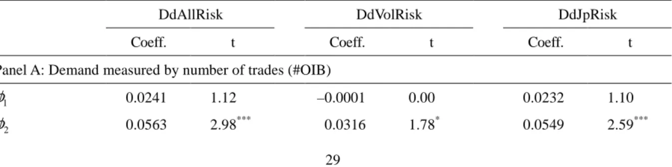
Table 7 The effect of option demand pressure on VRP by controlling on option liquidity 28 Table 8 The demand effect of option based on the MA(1)-filtered returns ... 29

Table 9 Parameter Estimates for the VAR Model in Equation (9) ... 44

Table 10 Summary Statistics ... 47

Table 11 Adjustment of Time Series Data ... 50

Table 12 Ordinary Least Squares Regression Coefficients... 51

Table 13 Results of Linear Granger Causality Test... 53

Table 14 Results of Nonlinear Granger Causality Test ... 56

Table 15 Results of Pairwise Nonlinear Granger Causality Test... 57

Table 16 Pairwise Nonlinear Causality Tests after Controlling of Information Flows ... 60

Table 17 OLS Coefficients Distinguishing Overnight Observations... 62

Table 18 Results of Pairwise Nonlinear Granger Causality Test without Overnight Observation ... 64

LIST OF FIGURES

Figure 1 Time series plots of implied volatility, expected realized volatility, and volatility risk premium. ... 20

Figure 2 Time Series Plots of the Daily Risk-Neutral Volatility and Expected Realized Volatility... 45

Figure 3 Time Series Plots of Absolute Deviations from Median Volatility Risk Premium.46 Figure 4 Intraday Pattern of |dVRP| by Day of the Week. ... 48

(9)

1 CHAPTER 1 INTRODUCTION

Volatility risk premium (VRP) is the premium that compensates risk stemming from the fluctuation in volatility or jumps. Empirical research also provides strong evidence that this risk premium is priced in options. One interpretation within the most existing literature is that investors who purchase options need to pay a premium for protection against volatility risk. Along this line, the VRP is linked with expected future volatility, hedging demand, and liquidity provision. However, in practice, to meet the obligation of the liquidity provision, market makers must take on the other side of the end-user net demand. This gives a rise to an interesting but less understood question whether the VRP is determined by the option net demand of end users.

In addition, over the past few years, volatility trading has become increasingly popular. A large volatility risk premium provides opportunities to engage in volatility trading. In real market, the VRP is often substantial and implies large profits for option sellers (Eraker, 2008). Despite the overwhelming evidence that large volatility increases VRP, much is unknown about what happens afterward, in particular how a widened VRP may affect subsequent volatility. Therefore, this dissertation focuses on two important issues regarding the VRP in financial market.

The first issue in this dissertation is to discuss the impact of option demand pressure on volatility risk premium. Instead of using actual but unobserved option net demand, the order imbalance in the options is used because this measure is easily observable from public order flows and the result based on this demand measure allows liquidity providers to quickly adjust their bid-ask quote of options.

This paper calculates two types of order imbalance measures, one in number of trades and the other in traded dollar amount. For each order imbalance measure, three order imbalance variables are calculated separately weighted by three unhedgeable risks for

(10)

market makers that correspond to aggregate risk, volatility risk, and jump risk. They are proxies for three demand variables for options: all demand, volatility demand, and jump demand. Each of these order imbalances variables is applied to examine the demand pressure effect on VRP.

The VRP is quantified as risk-neutral volatility less expected realized volatility. For the risk-neutral volatility, it is calculated directly from option prices using the approach proposed by Jiang and Tian (2005, 2007). Following Busch, Christensen, and Nielsen (2011) and Bollerslev and Todorov (2011), the expected realized volatility is estimated using a vector heterogeneous autoregressive model. Specifically, the estimate for VRP relies on two recently developed model-free measures: realized volatility and implied volatility. Using these two model-free measures, it is not only to calculate VRP easily but also has the advantages of the unspecified volatility process and pricing kernel.

Our empirical results show that the level of demand for an index option plays a key role in determining the time variation in VRP. In particular, as market jumps occur, the demand pressure leads to a greater impact on VRP for all three demand variables.

The second issue is to investigate the dynamic processes between VRP and volatility while focusing on the afterward effect of a large VRP. This study argues that a large VRP attracts volatility trading and is accompanied by hedging transactions, which could subsequently raise market volatility, resulting in a feedback effect that further enlarges market volatility. The bidirectional causality between VRP and market volatility is tested in 5-minute frequency using OLS regression, linear Granger causality, and nonlinear Granger causality tests. A traditional linear Granger causality model is applied to estimate the dynamic relationship between VRP and the realized volatility. The nonlinear causal test adopts a nonparametric method based on the modified version of the Baek and Brock (1992) nonlinear Granger causality test.

(11)

3

show significant two-way impact between realized volatility and VRP. The causal relation from VRP to the realized volatility suggests that VRP plays an important role in explaining future realized volatility: a large volatility premium could lead to greater realized volatility.

This study further separates the market volatility into three components: continuous volatility, negative jump volatility, and positive jump volatility, and examines the causality between VRP and each volatility component. In the nonlinear test, the VRP is found to Granger cause the three volatility components: continuous volatility, negative jump volatility, and positive jump volatility. This feedback effect that the VRP nonlinearly Granger causes the three volatility components is significant even after controlling for the higher volatility attributed to unexpected information shocks.

In conclusion, the dissertation gives some insights into the issues of the influence of option demand pressure on VRP and the effect of trading the VRP. The research results will offer us with the empirical evidence to comprehend the dynamic relationship between the demand pressure of index option and VRP, and between market volatility and VRP in financial market.

(12)

CHAPTER 2 THE IMPACT OF ORDER IMBALANCE IN OPTIONS ON VOLATILITY RISK PREMIUM: EVIDENCE FROM THE TAIWAN INDEX OPTION MARKET

1. INTRODUCTION

Recent literature documents that volatility risk stemming from the fluctuation in volatility is compensated by volatility risk premium (VRP) and priced in options.1 One economic interpretation within the most literature is that investors who purchase options are willing to pay a premium for protection against volatility risk. Several studies also show that the VRP represents option market makers’ willingness to absorb inventory and provide liquidity (Bollen, & Whaley, 2004; Gârleanu, Pedersen, & Poteshman, 2009; Nagel, 2012). Along these lines, the magnitude of VRP depends upon investors’ demand for hedging volatility risk and intermediaries’ willingness to meet the liquidity demand. Despite the abundant evidence has linked the VRP to liquidity, intermediation, and hedging demand, much less is known about the effect of option net demand of end users on the time-varying VRP.2

Gârleanu, Pedersen, and Poteshman (2009) propose a demand-based model in which the equilibrium option price is partly determined by its demand. The model shows that demand pressure for an option increases its price by an amount proportional to option’s expensiveness, i.e., the premiums of all unhedgeable risk of options such as discrete-time trading, volatility risk, and jump risk. It also raises the prices of other options on the same underlying proportional to the covariance of the unhedgeable parts. These results suggest that option demand impacts the VRP.

In addition, the demand pressure effect for VRP likely differs when risk aversion of

1_{See, for example, Bakshi and Kapadia (2003), Bollerslev and Todorov (2011), ; Buraschi and Jackwerth}

(2001), Carr and Wu (2009), Chernov and Ghysels (2000), Coval and Shumway (2001), and Jackwerth and Rubinstein (1996).

(13)

5

market participants varies because it may affect the willingness of market participants to buy or sell options. Todorov (2010) finds that time-varying risk aversion is mainly driven by large or extreme market moves. A large price shock to stock market increases investors’ fears for future jumps because investors view the occurrence of jumps as more likely, thereby raising their willingness to pay more for protection against jumps. At such time, it may result in a greater demand effect on VRP, especially when preceded by recent jumps, even through option demand remains the same or lessens. This matches the pattern of VRP in Todorov (2010): it increases and slowly reverts to its long-run mean after jumps occur. However, price jumps often appear in the most major market indices.3 This provides us a venue to test the differential effect of demand pressure on VRP with and without jumps.

This study investigates the effect of option demand pressure on VRP and test whether the demand pressure effect is greater when market jumps occur. The order imbalance in options is used instead of actual option net demand to analyze the demand pressure effect because this measure is easily observable from public order flows and the result based on this demand measure can be applied to adjust the bid-ask quote of options for liquidity providers. A finding that the order imbalances positively affect VRP with and without market jumps, with former having a larger impact, provides evidence that option demand pressure influences the VRP. To the best of our knowledge, this study is the first of its kind to investigate the dynamic relation between option demand pressure and VRP. Our study contributes to the existing literature not only by illustrating the importance of demand pressure in determining VRP but also by explicitly linking the demand pressure effect on VRP with time-varying risk aversion.

The Taiwan index options (TXO) written on the Taiwan Stock Exchange Capitalization Weighted Stock Index (TAIEX) are analyzed, in which TXO is one of the most liquid index

3_{Indeed, most major market indices appear to contain price jumps (Bakshi, Cao, and Chen, 1997; Bollerslev}

(14)

options in the world.4 The trading volume by individuals far exceeds the levels of trading by domestic or foreign institutional investors.5 The dominance by individual investors contrasts with the common knowledge that institutional investors dominate the index option market such as the U.S. market. Our study in the Taiwan market sheds light on many other markets at a similar stage of development such as Korea and Poland.

To meet the obligation of the liquidity provision, market makers must take on the other side of the end-user net demand. If market makers can not perfectly hedge their net exposure on the option positions, the option prices that they quote include a component that compensates their risk. In real world, the risks faced by market makers stem from incomplete markets such as transaction costs, discrete-time transaction, unexpected volatility, and sudden jumps in the underlying price. Market makers who accept these unhedgeable risks thus require a premium for providing liquidity on option markets. Gârleanu, Pedersen, and Poteshman (2009) and Bollen and Whaley (2004) find that the option’s expensiveness is related to the level of risk taken on by the market makers.

The order imbalances are used to proxy for option net demand. Many studies show that order imbalances between buyers and sellers can reflect nonmarket maker net demand. Chordia, Roll, and Subrahmanyam (2002) and Chordia and Subrahmanyam (2004) use order imbalance to measure both direction and degree of buying or selling pressure. Bollen and Whaley (2004) gauge net demand using order imbalances between the number of buyer-initiated and seller-initiated trades. More important, in contrast to the end-user net demand identified with a unique data set by Gârleanu, Pedersen, and Poteshman (2009) and Ni, Pan, and Poteshman (2008), this demand measure is quickly observed from public order flows.

4_{On a global scale, the TXO is ranked the fifth most frequently traded index option in 2010.}_{The constituent}

stocks of the underlying spot index are also actively traded.

(15)

7

This study follows Chordia, Roll, and Subrahmanyam (2008) to calculate two types of order imbalance measures, one in number of trades and the other in traded dollar amount. For each order imbalance measure, three order imbalance variables are calculated separately weighted by three unhedgeable risks for market makers that correspond to aggregate risk, volatility risk, and jump risk. They are proxies for three demand variables for options: all demand, volatility demand, and jump demand. Each of these order imbalances variables is applied to examine the demand pressure effect on VRP.

The VRP is quantified as risk-neutral volatility less expected realized volatility. For the risk-neutral volatility,it is calculated directly from option prices using the method proposed by Jiang and Tian (2005, 2007). Following Busch, Christensen, and Nielsen (2011) and Bollerslev and Todorov (2011), the expected realized volatility is estimated using a vector heterogeneous autoregressive (VecHAR) model. Specifically, the estimate for VRP relies on two recently developed model-free measures: realized volatility and implied volatility. Using these two model-free measures, it is not only to calculate VRP easily but also has the advantages of the unspecified volatility process and pricing kernel.6

Our empirical results show that the level of demand for an index option plays a key role in determining the time variation in VRP. In a time-series test, a positive influence of option demand pressure on VRP is found, similar to the finding of Gârleanu, Pedersen, and Poteshman (2009) that a proportion of an option’s expensiveness reflects the effect of demand pressure. The finding of a strong linkage between demand pressure and VRP during the period of recent market-maker losses indicates that demand pressure effect is related to the risk aversion of liquidity providers. In particular, when market jumps occur, the demand pressure leads to a greater impact on VRP for all three demand variables. The result provides evidence to support the finding of Todorov (2010) that time-varying risk aversion is driven

6_{For example, utilizing the joint estimation of the asset returns and prices of its underlying derivatives}

requires complicated modeling and estimation procedures (Ait-Sahalia & Kimmel, 2007; Bates, 1996; Chernov & Ghysels, 2000; Eraker 2004; Jackwerth, 2000; Jones, 2003; Pan, 2002).

(16)

by large, or extreme, market moves.

The remainder of this paper is organized as follows. Section 2 contains the formal development of our method. Section 3 provides a brief description of the empirical data. Section 4 analyzes the empirical results. Section 5 provides the key results of the study and a conclusion.

2. METHODOLOGY

2.1. Volatility Risk Premium

VRP represents the premium associated with uncertainty in volatility and is often measured by the difference between the statistical and risk-neutral expectations of the forward variation in the asset return. To measure VRP faced by liquidity providers, this study follows Bollerslev and Todorov (2011) and Todorov (2010) and define VRP over the next τ trade days as the risk-neutral volatility less the expected realized volatility, quantified as [ , ] [ , ] 1/ . Q( ) 1/ . P( ), t t t t t t t VRP =

τ

E

σ

₊_τ −

τ

E

σ

₊_τ (1) where Q(.) E and P(.)

E indicate the expectations under risk-neutral and statistical measures, respectively.7

2.1.1. Estimate of risk-neutral volatility

The risk-neutral volatility at the first term in Equation (1) is calculated directly from option prices. As demonstrated in Bakshi and Madan (2000), Britten-Jones and Neuberger

7_{Note that our VRP measure in Equation (1) is opposite to the definition of Bollerslev and Todorov (2011)}

(17)

9

(2000), and Jiang and Tian (2005), this risk-neutral volatility is equal to option implied volatility. In this study, the approach proposed by Jiang and Tian (2005, 2007) is adopted to compute the implied volatilities of call and put options directly from option prices. This method corrects the inherent methodological problem in the most widely used Black– Scholes (1973) model for deriving the option-implied volatility, which assumes that the underlying asset’s return follows a lognormal distribution that is virtually found to be too fat-tailed to be lognormal.

Britten-Jones and Neuberger (2000) derive a model-free measure of implied volatility under the diffusion asset price process, and Jiang and Tian (2005) further extend their result to the case of jump diffusion. The model-free implied variance is defined as an integral of option prices over an infinite range of exercise prices, denoted as

0 2 0 ( , ) max(0, ) 2 C K F K dK K τ ∞ − −

∫

F , in which the superscript F denotes the forward probability measure, K is the exercise price,

τ

denotes the time to maturity, F0 and CF( ,

τ

K) are the

forward asset and option prices.

However, in reality, options are trades in the marketplace only over a finite range of exercise prices. The limited availability of discontinuous exercise prices may lead to truncation and discretization errors in the numerical integration for the model-free implied volatility.8 To resolve the problem, Jiang and Tian (2005, 2007) develop an interpolation– extrapolation scheme to reduce the influence of truncation and discretization errors.9

8_{The truncation error results from disregarding exercise prices beyond the range of the listed exercise prices}

in the marketplace, and the discretization error arises from the discontinuous exercise prices. In general, the truncation error is negligible while the truncation points are more than two standard deviations from the forward asset price (Jiang & Tian, 2005).

9_{The steps are specified as follows. At first, a wider range of exercise prices relative to available exercise}

prices is set up by given left and right truncation points Kmin and Kmax. Next, to obtain the not-traded option

prices between these two truncation points, a cubic splines method is used to interpolate the Black–Scholes implied volatilities per the ∆K price interval between available exercise prices. Finally, the extracted implied volatilities are translated into option prices by using the Black–Scholes model, and the implied volatility is further computed from these option prices. In addition, for options with exercise prices beyond the available range in option market, Jiang and Tian suggest that the slope of the extrapolated segment (on both sides) should be adjusted to match the corresponding slope of the interior segment at the minimum or maximum available exercise price.

(18)

Following the approach of Jiang and Tian (2005, 2007), the model-free implied variance is written as ax min 0 1 2 1 ( , ) max(0, ) 2 m ( ( , ) ( , )) , M K j j K j C K F K dK f K f K K K

τ

_τ

− = − − ₌

_∑

₊ _∆

∫

F (2)

where f( ,τ K_i)=(CF( ,τ K) max(0,− F₀−K_i)) /K_i2, ∆K = (Kmax–Kmin)/M, Ki = Kmin+ i∆K

for 0≤i≤M. The truncation interval [Kmin, Kmax] denotes the range of available exercise

prices, in which Kmin and Kmax are referred as left and right truncation points, respectively.

In our empirical work, option and asset prices are used instead of forward prices to calculate the implied volatility. Under the assumption of deterministic interest rate, the forward option price and forward asset price at time t are respectively represent as CF( ,τ K)=C( ,τ K) / ( , )B t τ _and

/ ( , ) t t

F =S B t τ , in which S is spot price, _t C( ,τ K)is the option price, and B t( , )τ is the time t price of a zero-coupon bound that pays $1 at time τ.

To avoid the bid–ask bounce problem, the midpoint of the quote rather than the transaction price is used to compute the implied volatility (Bakshi, Cao, and Chen, 1997, 2000). As calculating the implied volatility in Equation (5), this study truncates the integration at the lower and upper bounds of 95% and 140% of the current index price for call options and of 60% and 105% of the current index price for put options. The ∆K in numerical integration scheme of Equation (2) is set as 20 index points.10

In each day, the implied volatilities at the nearest two maturities are linearly interpolated to obtain the implied volatility at a fixed 22 trading-day horizon. For the implied volatility at each contract month, the average implied volatility of call and put is

10_{The strike price intervals of TXO stipulated by the TAIFEX are grouped into three categories. First, when a}

strike price is below 3,000 points, the strike price intervals are 50 points in the nearby month and the next two calendar months and 100 point intervals for all months in excess of two months in distance. Second, when a strike price is between 3,000 and 10,000 points, the strike price intervals are 100 points in the nearby month and the next two calendar months, and 200-point intervals for far months. Third, when a strike price is over 10,000 points, the strike price intervals are 200 points in the nearby month and the next two calendar months,

(19)

11

first calculated every five-minute interval and then averaged across intervals in a day. The five-minute implied volatility of the call (and put) is backed out from call (put) prices by using Equation (2).

2.1.2. Estimate of expected realized volatility

The expected realized volatility at the second term in Equation (1) is estimated using a VecHAR model constructed on the volatility components of model-free realized volatility. Andersen, Bollerslev, and Diebold (2007) find that the forecasting to the future realized volatility improves significantly when using continuous volatility (CV) and jump volatility (JV) decomposed from realized volatility as separate regressors. They show that volatility components provide better forecasting than realized volatility itself because of the distinct features associated with the CV series and JV series: CV is strongly serially correlated while JV is less persistent and far less predictable than CV. The different features for the two components indicate separate roles in the forecast of realized volatility. In addition, Barndorff-Nielsen and Shephard (2001), Bollerslev, Kretschmer, Pigorsch, and Tauchen (2009), and Todorov and Tauchen (2006, 2011) find that the future volatility increases more following negative price jumps.

Following the Bollerslev and Todorov (2011), the daily close-to-close realized volatility is decomposed into four parts with different characteristics: overnight volatility (NV), CV, nJV, and pJV. In brief, the daily realized volatility is first calculated using 5-minute intraday returns and then decomposed it into four volatility components. This process produces four daily series, one for each volatility component, CV, nJV, pJV, and NV.

(20)

(2011)11 is applied to forecast the one-period ahead of volatility components. The model follows Andersen et al. (2007) to contain daily, weekly, and monthly volatility measures in the VecHAR forecasting specifications. The expected realized volatility with a 22-day horizon is the square root of the relevant forecasts’ sum for the volatility components. The VecHAR model uses the four-dimensional vector Zt, consisting of the CV, nJV, pJV, and

NV estimated previously, as input:

22 0 1 1 5 5 22 22 22, ( ) ' t t t t t t t t t t Z B B Z B Z B Z Z CV nJV pJV NV ε + = + − + − + − + + = (3)

where Zt–1, Zt–5, and Zt–22, respectively, denote the vector of lagged daily, weekly, and monthly

volatility components. B0 is a vector of the intercept term. B1, B5, and B22 are matrices for the

regression coefficients, in which the first column, second column, third column, and fourth column in each matrix correspond to the parameters of the four volatility components, respectively. The model uses the past 800 days for the estimation of parameters B0, B1, B5,

and B22. The one-period-ahead volatility component vector is obtained using the estimated

parameters and the past 22 days’ volatility components. To produce daily-frequency forecasting, this study rolls forward daily, using the same window length (800 days) for every forecasting.

2.2. Option Demand Variables

The option net demand is measured using order imbalance in options. The order imbalance is defined as buyer-initiated trade minus seller-initiated trade, where the Lee and Ready (1991) algorithm is used to classify each option trade into buyer-initiated or seller-initiated trades.12 Following Chordia, Roll, and Subrahmanyam (2008), two types of

11_{Busch, Christensen, and Nielsen (2011) introduce a VecHAR model for the joint modeling the separate}

components of realized volatility to forecast volatility components. This model generalizes the heterogeneous autoregressive approach proposed by Corsi (2004) for realized volatility analysis and extended by Andersen et al. (2007) to include the separate volatility components of past realized volatility as regressors.

(21)

13

order imbalance measures are calculated: one in number of trades and the other in traded dollar amount. The order imbalance in trade #OIB is quantified as the difference between the number of buyer- initiated and seller-initiated trades divided by the total number of trades within every 5-minute interval. Dollar order imbalance $OIB is the total dollars paid by buyer-initiated trades less the total dollars received by seller-initiated trades divided by the dollars for all trades within every 5-minute interval.

For each order imbalance measure, three order imbalance variables are calculated separately weighted by three unhedgeable risks for market makers that correspond to aggregate risk, unexpected volatility, and sudden jumps in underlying price. They serve as proxies for option demand (DdAllRisk), volatility demand (DdVolRisk), and jump demand (DdJpRisk), respectively.

DdAllRisk places equal weights across all options and thus measures the aggregate risk demand. DdVolRisk captures the volatility risk-induced demand by weighting order imbalances across all options according to Black–Scholes’s vega. The vega reflects an option’s sensitivity to the changes in volatility. A large order imbalance in the high vega options indicates that traders are volatility buyers. Order imbalances averaged across option series using vegas as the weight would, therefore, represent demand due to increased volatility risk as documented in Gârleanu, Pedersen, and Poteshman (2009) and Ni, Pan, and Poteshman (2008). For daily measure of DdAllRisk and DdVolRisk, the variable for every 5-minute interval is first calculated and then averaged across intervals in a day.

DdJpRisk captures the jump risk-induced demand by weighting the 5-minute option demand (DdAllRisk) across all 5-minute intervals in one day using the implied volatility skew. The implied volatility skew for an index option, as documented in Bates (2000) and

the prevailing quote mid-point. Conversely, a transaction is regarded as a seller-initiated trade if it occurs under the prevailing quote mid-point. For trades occur exactly at the midpoint of the quote, a “tick test” is used whereby the trade is classified as buyer-(seller-) initiated if the sign of the last non-zero price change is positive (negative).

(22)

Pan (2002), reflects the risk of market jumps. Large implied volatility skew indicates that investors highly anticipate future market jumps. Thus, order imbalances weighted across all 5-minute intervals using implied volatility skew as the weight represent the demand due to increased jump risk. In addition, the implied volatility skew is gauged using the slope of option implied volatility, which is calculated by the out-the-money implied volatility, the average implied volatility of call and put with spot-to-exercise ratio beyond the (1.03, 0.97) range, less the at-the-money implied volatility.

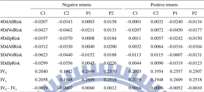
Table 1 provides the averages of daily order imbalances and implied volatilities of calls and puts in the negative and positive returns. A decline in the market price leads to negative order imbalances for near and second calls (C1 and C2, respectively) in each of the three demand variables and every order imbalance measure, and almost positive order imbalances for near and second puts (P1 and P2, respectively). This result indicates that investors have a preference for selling calls and buying puts when market price decreases. Inversely, they are inclined to buy calls and sell puts when market price increases. In addition, positive (negative) average order imbalances are found to increase (decrease) average volatility spread (IVd – IVa), which is the average difference in implied volatility between negative or

positive return period and the entire sample period. The increased (decreased) option price in respond to positive (negative) demand pressure provides evidence for the positive (negative) demand pressure effect on VRP, consistent with Gârleanu, Pedersen, and Poteshman (2009). For example, negative order imbalances in C1 and C2 (P1 and P2) decrease the option’s price about the size of 19 and 7 (52 and 10) basis-points, respectively, of implied volatility during the negative (positive) return period.

(23)

15

Table 1 Average order imbalances and option implied volatility

Negative returns Positive returns

C1 C2 P1 P2 C1 C2 P1 P2 #DdAllRisk –0.0207 –0.0343 0.0003 0.0158 –0.0001 0.0032 –0.0240 –0.0134 #DdVolRisk –0.0427 –0.0462 –0.0211 0.0131 –0.0207 0.0072 –0.0450 –0.0177 #DdJpRisk –0.0197 –0.0370 0.0008 0.0184 0.0011 0.0057 –0.0242 –0.0150 $DdAllRisk –0.0312 –0.0330 0.0040 0.0200 0.0032 0.0064 –0.0316 –0.0104 $DdVolRisk –0.0623 –0.0440 –0.0152 0.0188 –0.0113 0.0115 –0.0607 –0.0131 $DdJpRisk –0.0299 –0.0356 0.0045 0.0226 0.0044 0.0090 –0.0319 –0.0123 IVd 0.2040 0.1942 0.2669 0.2530 0.2075 0.1954 0.2557 0.2507 IVa 0.2058 0.1948 0.2609 0.2518 0.2058 0.1948 0.2609 0.2518 IVd – IVa –0.0019 –0.0007 0.0060 0.0012 0.0016 0.0006 –0.0052 –0.0010

Notes. This table reports average order imbalances and implied volatilities of call and put options separately corresponding to negative and positive returns. The data cover the period from January 1, 2005 to December 1, 2009. The order imbalances are measured by both the number of trades (#) and traded dollar amount ($). For each order imbalance measure, we calculate three order imbalance variables which correspond to aggregate risk, volatility risk, and jump risk, respectively. They serve proxies for aggregate demand, volatility demand, and jump demand. #DdAllRisk, #DdVolRisk, and #DdJpRisk ($DdAllRisk, $DdVolRisk, and $DdJpRisk) are the order

imbalances measured by the number of trades (traded dollar amount). C1 and P1 (C2 and P2) indicate near-month (second-month) call and put options. IVd is the average of implied volatility in respond to negative or positive

returns; IVa is the average implied volatility during all the sample period. The difference in implied volatility, IVd –

IVa, indicates the volatility spread.

In addition, to simplify our analysis, we aggregate the demand of call and put options with the same exercise price and maturity in every 5-minute interval. Gârleanu, Pedersen, and Poteshman (2009) argue that linearly dependent derivatives have the same demand effect on option prices. If the put–call parity holds, the prices of a call and a put with the same exercise price and maturity must linearly related. Any demand pressure on the call (price increase) would similarly affect the put, causing the put price to increase.

2.3. Model Specifications

2.3.1. Testing the effect of option demand pressure on VRP

The regression model of Chan and Fong (2006) and Giot, Laurent, and Petitjean (2010) is adopted to assess the impact of demand pressure on VRP. VRP is regressed against a Monday dummy (MD), twelve lags for VRPs, and two option order imbalances in the near and second months (OIB₁,OIB₂, respectively). The t-statistics of estimated parameters are

(24)

calculated using the Newey and West (1987) standard errors.

In addition, two types of order imbalance measures are used to proxy for option net demand: one in number of trades (#OIB) and the other in traded dollar amount ($OIB). For every order imbalance measure, three order imbalance variables are calculated to separately proxy for all demand (DdAllRisk), volatility demand (DdVolRisk), and jump demand (DdJpRisk). The three order imbalance variables are used to test for the demand pressure effect on VRP in the presence of the sources of unhedgeable risk. Each of them is individually included in the regression model of Equation (4):

12 0 1 1, 2 2, 1 , m t t t t j t j t j VRP

α α

MD

φ

OIB

φ

OIB

ω

VRP₋

ε

= = + + + +

_∑

+ (4)

where MD is a Monday dummy variable that takes 1 for Monday, and zero otherwise. This dummy variable controls for the Monday effect.OIB and ₁ OIB respectively denote the ₂

daily option order imbalances in the near and second months. VRPt–js are lagged VRPs to

control for serial dependence in the VRP.

Further, this study illustrates whether the linkage between demand pressure and VRP is strong following market-maker losses. In reality, market makers are sensitive to risk due to the capital constraints, tolerance of leverage, and agency. If the risk aversion held by market makers plays a crucial role in determining the compensation for accommodating option demand, then the VRP would be expected to be sensitive to demand during their loss period. Following Gârleanu, Pedersen, and Poteshman (2009), the interaction between the market-maker profits and demand pressure, denoted as IntDdP&L, is used to gauge the demand pressure effect of recent profits and losses of market makers. The other control variables for the daily index return (IR) and daily realized volatility (RV) associated with option price (implied volatility) are also included into the regression model in Equation (5).

(25)

17 1 0 1 1, 2 2, 2 3 12 1 & , t t m t t t t t t j t j j IntDdP L VRP MD OIB OIB RV IR VRP β

α α

φ

β

ω

−

ε

= + = + + + + + +

∑

+ (5)

The daily IntDdP&L is calculated by the sum of product of lag daily market-maker hedged profits (P&Ls) and daily option net demand (DdAllRisk) in the near and second months. For each of call and put options in the near- and second-month, it is assumed to be sold or bought at the midpoint price of quotes. Further, price risk every 30 minutes is dynamically hedged to keep delta-neutral of option positions until option expiration date by buying or selling |delta| units of the underlying futures in the case of a call (put).13 In each contract month, the daily hedged profits (P&Ls) for market makers are calculated depending on the sign of order imbalance in a trade day. If the option net demand of end users (order imbalance) is positive, i.e., a sell demand for market makers, the daily P&Ls sum up the 30-minutes delta-hedged gains for all sold option series in a trade day. Similarly, for negative order imbalance, the daily P&Ls are sum of the 30-minutes delta-hedged gains for all bought option series in a trade day. In addition, RV, denotes realized volatility, is measured by the sum of the squared 5-minute returns in a day

2.3.2. Testing the effect of demand pressure with time-varying risk aversion

In addition to empirical evidences in favor of changes in risk aversion (e.g., Brandt and Wang, 2003), Todorov (2010) also finds that market jumps drive time-varying risk aversion. Large or extreme price moves increase both investors’ and market makers’ fear of future jumps. Immediately after the occurrence of jumps, investors are willing to pay a higher

13_{The delta is calculated by constructing on the Black–Scholes model, in which the implied volatility on day t}

is used to forecast the realized volatility on day t+1. Moreover, in our study, every TXO can be hedged only by a quarter of TXF contract because the multipliers for the futures and options contracts are NT$200 and NT$50 per index point, respectively.

(26)

premium for protection against jumps because they view the possibility of future jumps as more likely. However, most major market indices appear to contain price jumps. If risk aversion is indeed driven by jump activity, the demand pressure effect with jumps should result in a substantial impact on VRP in each of three demand variables.

To link the demand pressure effect with time-varying risk aversion, a jump dummy variable (D) is included in Equation (6). The nonparametric test proposed by Lee and Mykland (2008) is adopted to identify the price jumps. Dt is a dummy variable that is equal

to 1 if a price jump occurs during the daily trading time period on day t, and zero otherwise. Dt*OIBt captures the demand pressure effect in the occurrence of jumps. Here, it is

expected to be larger demand pressure effect for the three demand variables as jumps occur:

0 1 1, 2 2, 1 1, 2 2, 1 12 2 3 1 . * * & t m t d t t t t t t t t t j t j t j t

VRP MD D OIB OIB D OIB D OIB

RV IR VRP IntDdP L α α α φ φ ψ ψ β β β ω − ε = = + + + + + + + + + + +

∑

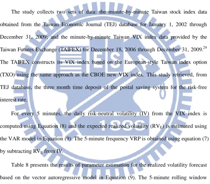
+ (6) 3. DATA

This study requires two sets of data. The intraday data on the Taiwan index option (TXO), which is traded on the TAIFEX14, are obtained from the Taiwan Economic Journal (TEJ) database. The data contain trade and quote files of options. The transaction prices, transaction volumes for every trade are extracted from the trade file and the bid and ask prices are acquired from the quote file for January 1, 2005 through December 31, 2009. The minute-by-minute Taiwan stock index data are also obtained from the TEJ database for January 1, 2002 through December 31, 2009.

Several data filters are applied to select our final sample. First, the options with a quote

14_{The TAIFEX introduced the European style TXO, written on the TAIEX, on December 24, 2001. The}

contract matures on the third Wednesday of the delivery month. The contract months involve five contracts with different maturities in the nearby month, the next two calendar months, and the following two quarterly

(27)

19

price of less than 0.1, the minimum tick size, are excluded. These prices cannot reflect true option value. Second, due to the potential liquidity concerns, the options with less than five trading days remaining to maturity are eliminated. Third, the options violating the put–call parity boundary conditions are deleted. These options are significantly undervalued and have negative Black–Scholes implied volatilities.

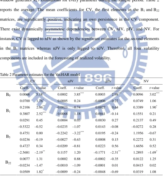
Table 2 presents the results of the parameter estimation for the realized volatility forecast based on the VecHAR model in Equation (3). The procedure of a daily rolling window generates 927 estimations for every parameter during the sample period. Table 2 reports the average. The mean coefficients for CV, the first elements in the B1 andB22

matrices, are significantly positive, indicating an own persistence in the CV component. There exist dynamically asymmetric dependencies between CV, nJV, pJV, and NV. For instance, CV is lagged to nJV as shown by the significant estimates for the second elements in the B1 matrices whereas nJV is only lagged to nJV. Therefore, all four volatility

components are included in the forecasting of realized volatility.

Table 2 Parameter estimates for the VecHAR model

CV nJV pJV NV

Coeff. t-value Coeff. t-value Coeff. t-value Coeff. t-value

B0 0.0068 5.18*** 0.0002 3.85*** 0.0003 2.98*** 0.0096 3.02*** 0.0700 1.76* 0.0005 0.24 –0.0006 –0.27 0.0749 1.06 0.2106 2.06** –0.0023 –0.74 0.0027 0.64 0.3389 1.90* 0.3807 2.52*** 0.0068 1.18 0.0041 –0.14 0.1551 0.21 B1 0.0291 0.45 0.0004 0.03 0.0030 0.27 0.2137 0.49 –0.5322 –0.52 –0.0235 –1.07 0.0143 –0.08 –0.0272 0.28 0.4751 0.00 –0.2242 –3.22*** 0.0195 –0.24 1.1956 –0.67 0.0236 –0.19 –0.0027 –0.63 0.0008 0.15 0.2272 0.31 B5 0.4727 0.34 –0.0209 –0.81 0.0223 0.56 1.6656 0.52 –2.5681 –2.19** 0.1157 1.20 –0.1771 –2.31** 1.2893 –1.69* 0.0077 1.31 0.0002 0.88 –0.0002 –0.35 0.0122 1.25 –0.0234 –1.47 –0.0010 –1.09 –0.0001 0.01 0.0415 0.02 B22 0.0509 1.82* –0.0009 –0.24 –0.0048 –0.69 0.0319 1.08

(28)

Notes. This table presents the estimating results of parameters for realized volatility forecast based on a vector autoregressive (VecHAR) model in Equation (3):

22 0 1 1 5 5 22 22 22, ( ) '. t t t t t t t t t t Z B B Z B Z B Z Z CV nJV pJV NV ε + = + − + − + − + + = (3) The expected realized volatility is estimated using the moving window data of past 800 days. The realized variation measures underlying the estimate are based on 5-minute high-frequency data from January 1, 2002 to December 31, 2009 inclusively. The procedure of a daily rolling window generates 927 estimations for each parameter during the sample period.Table 2 reports the average. In Equation (3), B0 is a vector of the intercept

term. B1, B5, and B22 are matrices for the regression coefficients, in which the first column, second column,

third column, and fourth column in each matrix correspond to the parameters of the four volatility components, respectively. A four-dimensional vector is included in the VecHAR model, involving continuous volatility (CV), negative jump volatility (nJV), positive jump volatility (pJV), and overnight volatility (NV). In addition, Newey–West standard errors are used to calculate the t-values of the estimated parameters. Coeff. indicates the regression coefficient. ***, **, and * indicate that t-values are significant at the 0.01, 0.05, and 0.1 level, respectively.

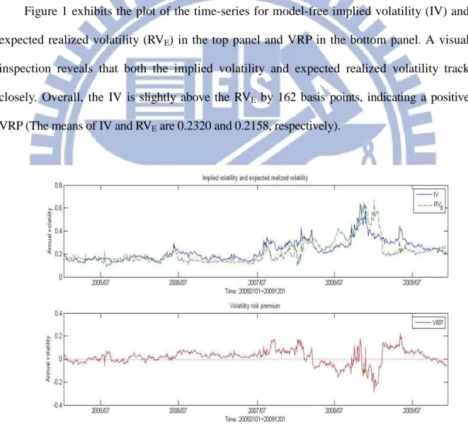
Figure 1 exhibits the plot of the time-series for model-free implied volatility (IV) and expected realized volatility (RVE) in the top panel and VRP in the bottom panel. A visual

inspection reveals that both the implied volatility and expected realized volatility track closely. Overall, the IV is slightly above the RVE by 162 basis points, indicating a positive

VRP (The means of IV and RVE are 0.2320 and 0.2158, respectively).

Figure 1. Time series plots of implied volatility, expected realized volatility, and volatility risk premium. The volatility risk premium (VRP) is quantified as the model-free implied volatility (IV) less the expected realized volatility (RVE). The model-free method proposed by Jiang and Tian (2005, 2007) is adopted to extract the

(29)

21

The second panel of Figure 1 shows that the time-series VRP ranges from –0.2883 to 0.2245 during the period of 2005–2009 and has a mean 0.0162. The 1.62% volatility spread provides evidence to support the finding of Bollen and Whaley (2004) and Gârleanu et al. (2009) that market makers who provide liquidity to the buy side are compensated for accepting risk.However, when the market is more volatile, market makers also face substantial risk of losses. In the period of financial crisis in 2008, a negative VRP, also shown in Todorov (2010) and Bollerslev, Gibson, Zhou (2011), occurs frequently. That is, market makers providing liquidity to the buy side suffer trading losses. In addition, the VRP is stationary time series according to the results of the Dickey–Fuller test with test statistic of -44.6.

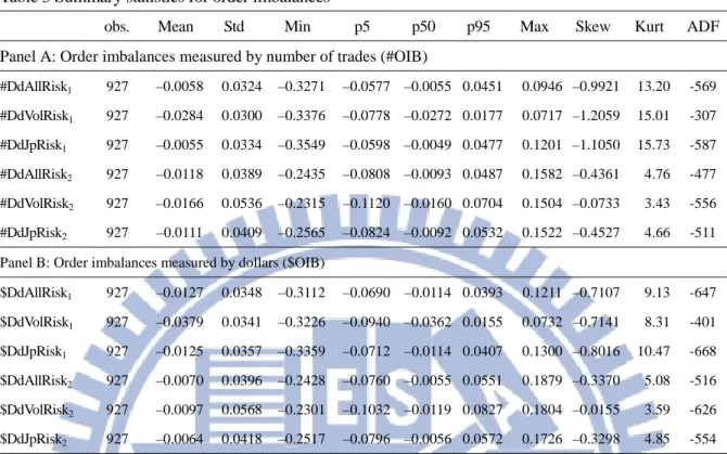
Panels A and B of Table 3 respectively report the summary statistics of option order imbalances measured by the number of trades (#OIB) and traded dollar amount ($OIB). #DdAllRisk1, #DdVolRisk1, and #DdJpRisk1 (#DdAllRisk2, #DdVolRisk2, and #DdJpRisk2)

indicate option demand, volatility demand, and jump demand in the near (second) month, in which all are measured by the number of trades. Similarly, $DdAllRisk1, $DdVolRisk1, and

$DdJpRisk1 ($DdAllRisk2, $DdVolRisk2, and $DdJpRisk2) are option demands in the near

(second) month measured by the dollars $OIB. The results show that all the option order imbalances are slightly negative, negative skewness, and leptokurtic. For instance, the DdAllRisk1, DdVolRisk1, and DdJpRisk1 measured by #OIB ($OIB) in the near month

average –0.0058, –0.0284, and –0.0055 (–0.0127, –0.0379, and –0.0125), respectively. In addition, the augmented Dickey–Fuller (ADF) unit root tests significant reject the hypothesis of one unit root for every individual series, indicating that these demand variables are stationary. The correlation coefficients between option order imbalances in near- and second-month for #DdAllRisk, #DdVolRisk, and #DdJpRisk ($DdAllRisk,

$DdVolRisk, and$DdJpRisk) are 0.09, 0.06, and 0.09 (0.18, 0.22, and 0.15), respectively. The

correlation coefficients range from 0.06 to 0.22, showing a low correlation between these option demand variables in the near- and second-month.

(30)

Table 3 Summary statistics for order imbalances

obs. Mean Std Min p5 p50 p95 Max Skew Kurt ADF Panel A: Order imbalances measured by number of trades (#OIB)

#DdAllRisk1 927 –0.0058 0.0324 –0.3271 –0.0577 –0.0055 0.0451 0.0946 –0.9921 13.20 -569 #DdVolRisk1 927 –0.0284 0.0300 –0.3376 –0.0778 –0.0272 0.0177 0.0717 –1.2059 15.01 -307 #DdJpRisk1 927 –0.0055 0.0334 –0.3549 –0.0598 –0.0049 0.0477 0.1201 –1.1050 15.73 -587 #DdAllRisk2 927 –0.0118 0.0389 –0.2435 –0.0808 –0.0093 0.0487 0.1582 –0.4361 4.76 -477 #DdVolRisk2 927 –0.0166 0.0536 –0.2315 –0.1120 –0.0160 0.0704 0.1504 –0.0733 3.43 -556 #DdJpRisk2 927 –0.0111 0.0409 –0.2565 –0.0824 –0.0092 0.0532 0.1522 –0.4527 4.66 -511

Panel B: Order imbalances measured by dollars ($OIB)

$DdAllRisk1 927 –0.0127 0.0348 –0.3112 –0.0690 –0.0114 0.0393 0.1211 –0.7107 9.13 -647 $DdVolRisk1 927 –0.0379 0.0341 –0.3226 –0.0940 –0.0362 0.0155 0.0732 –0.7141 8.31 -401 $DdJpRisk1 927 –0.0125 0.0357 –0.3359 –0.0712 –0.0114 0.0407 0.1300 –0.8016 10.47 -668 $DdAllRisk2 927 –0.0070 0.0396 –0.2428 –0.0760 –0.0055 0.0551 0.1879 –0.3370 5.08 -516 $DdVolRisk2 927 –0.0097 0.0568 –0.2301 –0.1032 –0.0119 0.0827 0.1804 –0.0155 3.59 -626 $DdJpRisk2 927 –0.0064 0.0418 –0.2517 –0.0796 –0.0056 0.0572 0.1726 –0.3298 4.85 -554 Notes. This table presents summary statistics for daily option order imbalances in the near and second months. Panel A and Panel B report the statistics of order imbalances measured by number of trades (#OIB) and dollars ($OIB), respectively. #DdAllRisk1, #DdVolRisk1, and#DdJpRisk1 (#DdAllRisk2, #DdVolRisk2, and#DdJpRisk2) indicate

option demand, volatility demand, and jump demand in the near (second) month, in which order imbalances are measured by the number of trades. Similarly, $DdAllRisk1, $DdVolRisk1, and $DdJpRisk1 ($DdAllRisk2,

$DdVolRisk2, and$DdJpRisk2) are option demands in the near (second) month, in which they are measured by the

dollars $OIB. ADF is the augmented Dickey–Fuller unit root test.

4. EMPIRICAL RESULTS

4.1. Option Demand Pressure on VRP

In practice, the price of the option that market makers sell (buy) includes (excludes) risk premiums that compensate the unhedgeable risk. A positive (buy) demand pressure, which is opposite to the sell demand pressure for market makers, raises VRP, whereas a negative (sell) demand pressure decreases VRP. Thus, if demand pressure in an option affects VRP, it is expected to be a positive effect of demand pressure on VRP.

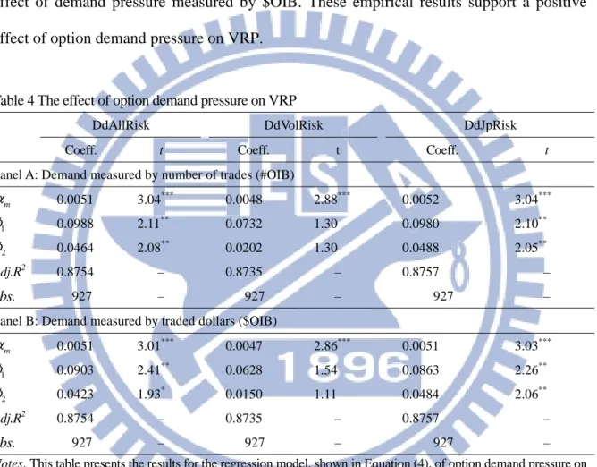
Panels A and B of Table 4 report the results of the demand effect measured by #OIB and $OIB, respectively. In Panel A, the coefficients for

φ

₁ and

φ

₂ in the near and second

(31)

23

months are both significant and positive for option demand (DdAllRisk) and jump demand (DdJpRisk). This finding indicates that demand pressure stemming from aggregate option demand and jump demand positively affects VRP. However, the volatility demand (DdVolRisk) pressure has relatively weak influence on VRP due to the positive but insignificant coefficients for

φ

₁ and

φ

₂. Panel B reports similar results for the positive effect of demand pressure measured by $OIB. These empirical results support a positive effect of option demand pressure on VRP.

Table 4 The effect of option demand pressure on VRP

DdAllRisk DdVolRisk DdJpRisk

Coeff. t Coeff. t Coeff. t

Panel A: Demand measured by number of trades (#OIB)

m α 0.0051 3.04*** 0.0048 2.88*** 0.0052 3.04*** 1 φ 0.0988 2.11** 0.0732 1.30 0.0980 2.10** 2 φ 0.0464 2.08** 0.0202 1.30 0.0488 2.05** Adj.R2 0.8754 – 0.8735 – 0.8757 – obs. 927 – 927 – 927 –

Panel B: Demand measured by traded dollars ($OIB)

m α 0.0051 3.01*** 0.0047 2.86*** 0.0051 3.03*** 1 φ 0.0903 2.41** 0.0628 1.54 0.0863 2.26** 2 φ 0.0423 1.93* 0.0150 1.11 0.0484 2.06** Adj.R2 0.8754 – 0.8735 – 0.8757 – obs. 927 – 927 – 927 –

Notes. This table presents the results for the regression model, shown in Equation (4), of option demand pressure on volatility risk premium (VRP).

12 0 1 1, 2 2, 1 , t m t t t j t j t j VRP α α MD φOIB φOIB ωVRP₋ ε = = + + + +

∑

+ (4)

Two types of option order imbalance are used to measure the option net demand, one in number of trades (#OIB) and the other in dollars ($OIB). The results are reported in Panel A and Panel B, respectively. For each type of order imbalance measure, three order imbalance variables are calculated separately weighted by aggregate risk, volatility risk, and jump risk and are used to proxy, respectively, for option demand (DdAllRisk), volatility demand (DdVolRisk) and jump demand (DdJpRisk). They are individually included in the regression model to investigate the demand pressure effect on VRP. The dependent variable, VRP, is quantified as the model-free implied volatility less expected realized volatility. OIB and ₁ OIB denote the daily option order imbalances in ₂ the near and second months, respectively. MD is a Monday dummy and the VRPt-j’s are lagged volatility risk

premiums. Newey–West standard errors are used to calculate the t-statistics of the estimated parameters. For brevity, this table does not report α⌢ and ₀ w⌢_j. ***, **, and * indicate that t-values are significant at the 0.01, 0.05, and 0.1 level, respectively.

(32)

DdJpRisk explain VRP better than DdVolRisk. A possible cause for the weak volatility demand pressure effect is that market makers ask for smaller compensation to take the relatively small volatility risk associated with small price moves. In addition, the significant and positive coefficients for dummy variable

α

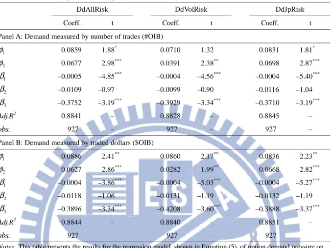
_m in both Panels A and B confirm the Monday effect (i.e., VRP is greater on Monday). The Monday effect may result from the accumulation of information over the weekend nontrading period. The high uncertainty during weekend may increase demand for using options to adjust the portfolios against volatility risk or jumps and subsequently causes higher VRP on Monday.

Table 5 provides the results of demand pressure effect by controlling on interaction between recent market-maker hedged profits and demand pressure (IntDdP&L), daily realized volatility (RV), and daily index return (IR). As shown in Panels A and B,

φ

₁ and

φ

₂ are almost significant positive for the three demand variables. This evidence makes it clear that demand pressure has a positive impact on the level of VRP regardless of the sources of unhedgeable risk. In addition, all the β1 coefficients are found to be significant negative in Panel

A and Panel B. The negative coefficients on the interaction between market-maker hedged profits and option net demand indicate an increase (decrease) in the demand pressure effect on VRP following recent market-maker losses (profits). Facing the trading loss, market makers with risk aversion ask a higher risk premium for accepting additional risk, consistent with Gârleanu, Pedersen, and Poteshman (2009) who find strong linkage between demand pressure effect and risk aversion. The result also provides evidence in supportive to that market makers play a crucial role in determining VRP.

The negativecoefficients for

β

₃ in Panels A and B suggest that a negative return may lead to higher VRP because investors are willing to pay more to hedge the potential decline than to hedge a possible increase.

(33)

25

Table 5 The effect of option demand pressure on VRP with control variables

DdAllRisk DdVolRisk DdJpRisk

Coeff. t Coeff. t Coeff. t

Panel A: Demand measured by number of trades (#OIB)

1 φ 0.0859 1.88* 0.0710 1.32 0.0831 1.81* 2 φ 0.0677 2.98*** 0.0391 2.38** 0.0698 2.87*** 1 β –0.0005 –4.85*** –0.0004 –4.56*** –0.0004 –5.40*** 2 β –0.0109 –0.97 –0.0099 –0.90 –0.0116 –1.04 3 β –0.3752 –3.19*** –0.3929 –3.34*** –0.3710 –3.19*** Adj.R2 0.8841 – 0.8828 – 0.8845 – obs. 927 – 927 – 927 –

Panel B: Demand measured by traded dollars ($OIB)

1 φ 0.0886 2.41** 0.0860 2.17** 0.0836 2.23** 2 φ 0.0627 2.86*** 0.0282 1.99** 0.0668 2.82*** 1 β –0.0004 –3.86*** –0.0004 –5.03*** –0.0004 –5.27*** 2 β –0.0118 –1.06 –0.0131 –1.19 –0.0132 –1.19 3 β –0.3896 –3.34*** –0.4208 –3.60*** –0.3888 –3.37*** Adj.R2 0.8844 – 0.8840 – 0.8851 – obs. 927 – 927 – 927 –

Notes. This table presents the results for the regression model, shown in Equation (5), of option demand pressure on volatility risk premium (VRP) by controlling on the interaction between market-maker hedged profits and option net demand (IntDdP&L), daily realized volatility (RV), daily index return (IR), and lagged VRPs:

12 0 1 1, 2 2, 1 2 3 1 . & t m t t t t t j t j t j t

VRP α α MD φOIB φOIB βIntDdP L β RV β IR ωVRP− ε =

= + + + + + + +

∑

+ (5)

Two types of option order imbalance are used to measure the option net demand, one in number of trades (#OIB) and the other in dollars ($OIB). The results are reported in Panel A and Panel B, respectively. For each type of order imbalance measure, three order imbalance variables are calculated separately weighted by aggregate risk, volatility risk, and jump risk and are used to proxy, respectively, for option demand (DdAllRisk), volatility demand (DdVolRisk) and jump demand (DdJpRisk). They are individually included in the regression model to investigate the demand pressure effect on VRP. The VRP is quantified as the model-free implied volatility less expected realized volatility. OIB and₁ OIB denote the daily option order imbalances in the near and second ₂ months, respectively. IntDdP&L is the interaction between market-maker hedged profits and option net demand. MD is a Monday dummy. The VRPt-j’s are lagged volatility risk premiums. Newey–West standard

errors are used to calculate the t-statistics of the estimated parameters. For brevity, this table does not reportα⌢ ,₀ α⌢ , and _m w⌢_j. ***, **, and * indicate that t-values are significant at the 0.01, 0.05, and 0.1 level, respectively.

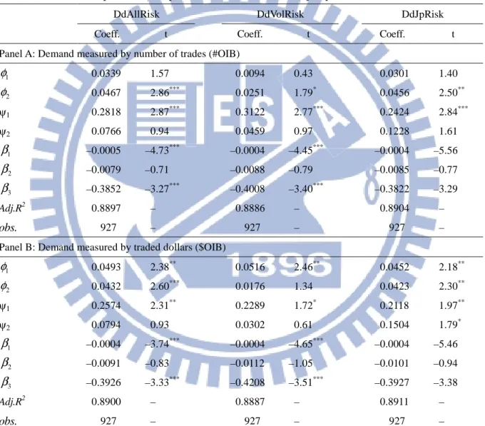
4.2. Option Demand Pressure on VRP with Time-Varying Risk Aversion

Table 6 reports the results of the demand pressure effect on VRP with jumps. All ψ1

coefficients in Panels A and B are significantly positive and larger than those for φ₁ for all three demand variables (DdAllRisk, DdVolRisk, and DdJpRisk). This indicates a greater

波動風險溢酬之決定因素及交易波動風險溢酬的影響:以臺灣指數選擇權市場為例

國 立 交 通 大 學

財務金融研究所

博 士 論 文

波動風險溢酬之決定因素及交易波動風險溢酬的影響:

以臺灣指數選擇權市場為例

The determinant of volatility risk premium and the effect of trading volatility

risk premium: Evidence from the Taiwan index option market

研 究 生：陳清和

指導教授：鍾惠民 教授

謝文良 教授

波動風險溢酬之決定因素及交易波動風險溢酬的影響:

以臺灣指數選擇權市場為例

The determinant of volatility risk premium and the effect of trading volatility

risk premium: Evidence from the Taiwan index option market

國 立 交 通 大 學

財務金融研究所

博 士 論 文

A Disseration

Submitted to Graduate Institute of Finance

College of Management

National Chiao Tung University

in Partial Fulfillment of the Requirements

for the Degree of

Doctor of Philosophy

In

Finance

November 2013

Hsinchu, Taiwan, Republic of China

中 華 民 國 一 O 二 年 十一 月

波動風險溢酬之決定因素及交易波動風險溢酬的影響:

以臺灣指數選擇權市場為例

國立交通大學財務金融研究所博士班

中文摘要

The determinant of volatility risk premium and the effect of trading volatility

risk premium: Evidence from the Taiwan index option market

誌 謝

CONTENTS

LIST OF TABLES

LIST OF FIGURES

τ

σ

τ

σ

∫

τ

τ

τ

τ

τ

∑

∫

α α

φ

φ

ω

ε

∑

α α

φ

φ

β

β

ω

ε

∑

∑

φ

φ

φ

φ

∑

α

φ

φ

β

∑

國立交通大學

博士論文

研究生：陳清和

指導教授：鍾惠民教授

謝文良教授

國立交通大學

博士論文

中華民國一 O 二年十一月

誌謝

_τ

_τ

_∑

_∑