線性馬達運動系統在巨觀及微觀區下之摩擦力分析及補償

國 立 交 通 大 學

機械工程研究所

碩

士

論

文

線性馬達運動系統

在巨觀及微觀區下之摩擦力分析及補償

The Analysis and Compensation of Friction for a

Linear-Motor-Driven Motion Stage Under Macro and Micro

Dynamic Scale

研 究 生：周亨隆

指導教授：李安謙 教授

線性馬達運動系統

在巨觀及微觀區下之摩擦力分析及補償

The Analysis and Compensation of Friction for a Linear-Motor-Driven

Motion Stage Under Macro and Micro Dynamic Scale

研究生：周亨隆 Student：Heng-Lung Chou

指導教授：李安謙教授 Advisor：Dr. An-Chen Lee

國立交通大學

機械工程研究所

碩士論文

A Thesis

Submitted to Institute of Mechanical Engineering

College of Engineering

National Chiao Tung University

in partial Fulfillment of the Requirements

for the Degree of Master of Science

in

Mechanical Engineering

July 2004

Hsinchu Taiwan Republic of China

中華民國九十三年七月

線性馬達運動系統

在巨觀及微觀區下之摩擦力分析及補償

研究生：周亨隆 指導教授：李安謙教授

國立交通大學機械工程研究所

摘要

本文研究如何精密控制一個受摩擦非線性影響下的直線馬達驅動運動系

統。 研究中發現 LuGre 模型，在描述微觀區摩擦力行為存在有若干的

缺失，因此針對此區，提出了一個改善的磨擦力模型，以便更精準地預測

其行為。 並利用此改善後的模型設計一前饋式摩擦力補償器，實驗顯示

此摩擦力補償器在微觀區下明顯優於以LueGre 模型設計的補償器，且在

巨觀區時，兩者具有相同的性能。 另外在巨觀區的實驗當中，我們也加

入干擾觀測器消除一些系統的不確定性和外在的干擾，實驗也顯示系統的

性能獲得大大地提升，可是卻發現干擾觀測器在作定位控制時，會產生極

限循環而嚴重影響定位精度，因此本論文提供了一個避免干擾觀測器產生

極限循環的充分條件，並據此條件設計控制器參數。 可是這些參數往往

會降低系統的性能而減少實用性，故論文裡也提出了一個調適的機制既可

以維持系統的性能也可避免極限循環的發生。

The Analysis and Compensation of Friction for a

Linear-Motor-Driven Motion Stage Under Macro and Micro Dynamic Scale

Student：

Heng-Lung Chou

Advisor：Dr. An-Chen Lee

Institute of Mechanical Engineering

National Chiao Tung University

Abstract

This paper studies how to control a linear-motor-driven motion system under the effect of nonlinear friction. The LuGre model has drawbacks and can’t describe some friction phenomena under micro-dynamic scale. Therefore, a modified friction model which can actually describe those phenomena is proposed. Then, a feedforward type friction estimator designed from this model is used to compensate the friction, and the experimental results show the compensator based on the modified friction model is much superior to that based on the LueGre model in micro scale region but have the same performance in macro scale region. In addition, we also add disturbance observer into servo loop to cancel the effects of system uncertainty and other disturbance under macro-dynamic scale. The experimental results show disturbance observer can certainly improve the system performance. Nevertheless, disturbance observer generates limit cycles in regulating control, which serverly decreases positioning accuracy. Therefore, this thesis derives a sufficient condition for the absence of limit cycles and exploits the condition to design controller parameters. The parameters designed from the condition usually make the system performance very low, so this thesis also introduces an adaptive mechanism that not only maintains the system performance but also eliminates limit cycles.

致 謝

由衷感謝恩師李安謙教授這兩年的指導，尤其是老師研究的方法、清晰的思 路和洞察能力更是讓我受益良多。 感謝學長施禕迪博士，在和他合作共事中，提供我 不少寶貴的意見及珍貴的知識，也感謝洪榮煌學長能不時地解答我的問題。 也感謝實 驗室的同仁陳岳汶、詹孟璋及童一峰能陪我一起度過難關。 也感謝好友江明謙、張萬 財、陳以理、和侯人友能不時的給我打氣和鼓勵。 最後由衷感謝我的父親周漢儀、 母親李芙蓉及弟周明遙，要是沒有你們背後的支持和鼓勵，就沒有今日的論文和成 果。

TABLE OF CONTENTS

LIST OF FIGURES ... vi

LIST OF TABLES ... xi

C

HAPTER

1

G

ENERAL

I

NTRODUCTION

...

1

C

HAPTER

2

S

ETUP OF

E

XPERIMENTAL

S

YSTEM

... 4

2.1 Hardware setup ... 4

2.2 Calibration of fiber optic laser encoder (RLE10) ………... 8

2.3 Modeling of the linear-motor-driven system ………... 9

2.4 The Dynamic LuGre model... 11

2.5 Parameters identification ... 12

C

HAPTER

3

C

ONTROLLER

D

ESIGN

... 14

3.1 Disturbance observer design... 15

3.2 Feedforward control ... 20

3.3 Velocity loop design... 21

3.4 Position loop design ... 24

3.5 Comparison of the feedforward structures ... 25

3.6 Simulations of controlled system ... 29

3.6.1 Test commands ... 29

3.6.2 Control structures under testing and comparison ... 31

3.7 Experiments of various control structures ... 42

C

HAPTER

4

T

HE

L

IMIT

C

YCLES

I

NDUCED

B

Y

D

ISTURBANCE

O

BSERVER

... 50

4.1 Introduction ... 50

4.2 The sufficient condition for the absence of limit cycle caused by mutual effect between disturbance observer and quantization ... 51

4.3 Application in the motion control systems ... 58

4.4 Adaptive parameters mechanism... 63

4.5 Experimental results ... 65

4.6 Summery... 71

C

HAPTER

5

T

HE

M

ODIFIED

F

RICTION

M

ODEL

F

OR

M

OTION

C

ONTROL

I

N

P

RESLIDING

R

EGION

... 73

5.1 Introduction ... 73

5.2 Important Friction Phenomena in Presliding Region ... 74

5.3 LueGre model and Modified friction model... 79

5.4 Identifying the modified friction model’s parameters... 93

5.5 Experimental results ... 97

5.6 Conclusion ... 109

C

HAPTER

6

C

ONCLUSIONS AND

F

UTURE

W

ORK

... 110

6.1 Conclusions ... 110

6.2 Future work ... 110

LIST OF FIGURES

Fig. 2.1 The experimental linear-motor-driven motion system together with the

resolution calibration system ... 5

Fig. 2.2 The plot of linear motor (From [88])... 6

Fig. 2.3 The photo of experimental system... 7

Fig. 2.4 Cascade control structure of the AC servo system with field-oriented control [89] . 9 Fig. 2.5 Block diagram of the current controlled power converter [89] ...9

Fig. 3.1 Block diagram of the proposed feedforward control structure with a disturbance observer and two feedback-type compensators.. ... 16

Fig. 3.2 Block diagram of the proposed feedforward control structure with a disturbance observer and two feedforward-type compensators... 16

Fig. 3.3 Block diagram of the disturbance observer for compensation. ... 17

Fig. 3.4 The derivation of equivalence disturbance which comes from the plant uncertainty ... 19

Fig. 3.5 Block diagram of the feedforward structure... .20

Fig. 3.6 Block diagram of the velocity loop. ... 21

Fig. 3.7 Block diagram of the feedforward structure for position loop. ... 24

Fig. 3.8 Block diagrams of two feedforward control structures for the linear motor motion system. (a) The FF structure proposed in this study; (b) the FF structure proposed in reference [87]... 27 Fig. 3.9 Experimental comparison of the proposed feedforward control structure and

the one proposed by Ref. [87]. (a) The position command and responses of two different structures. (b) Solid line represents the tracking error of the proposed FF structure, and dash line represent tracking error of the structure

proposed in reference paper... 28 Fig. 3.10 Trajectory of x with _r1 A₁=1 mm and T_r =0.25sec. ... 30 Fig. 3.11 The trajectory of x_r2 with A₂ =2 mm and T_p =0.5s ... 30 Fig. 3.12 The tracking errors of the eight different control structures for the high-order

polynomial trajectory defined in Fig. 6.10. ... 34 Fig. 3.13 The friction and cogging force compensators are implemented in feedforward

form. Four performance indices are plotted versus the eight different control structures. The errors (performance indices) are defined as (a) E_{max_t},

(b) E_{rms_t}, (c) E_{max_p}, and (d) E_{rms_ p}... 35 Fig. 3.14 Simulations of Tracking errors of the eight different control structures for the

sinusoidal command defined in Fig. 6.11... 37 Fig. 3.15 The four control performance indices are plotted versus the eight different

control structures. The error (performance index) is defined as (a) E_{max_s}, (b) E_{rms_s}, (c) E_{max_r}, and (d) E_{rms_r}... 38 Fig. 3.16 Simulated tracking errors of the eight different control structures for the

command defined in Fig. 6.10. The friction and cogging force compensators are implemented in feedback forms... 40 Fig. 3.17 Four performance indices are plotted versus eight different control structures.

The error (performance index) is defined as (a) E_{max_t}, (b) E_{rms_t},

(c) E_{max_p}, and (d) E_{rms_p}. ... 41 Fig. 3.18 Experimental tracking errors of the eight different control structures for the

command defined in Fig. 6.10. The friction and cogging force compensators are implemented in feedforward forms. ... 44

Fig. 3.19 The control performance indices are plotted versus different control structures, where the error (performance index) is defined as (a) E_{max_t}, (b) E_{rms_t},

(c) E_{max_p}, and (d) E_{rms_p}. ... 45

Fig. 3.20 Experimental tracking errors of the eight different control structures for the sinusoidal command defined in Fig. 6.11... 46

Fig. 3.21 The control performance indices are plotted versus different control structures, where the error (performance index) is defined as (a)E_{max_s}, (b) E_{rms_s}, (c) E_{max_r}, and (d)E_{rms_r}... 47

Fig. 3.22 Experimental comparison of the tracking results for the feedforward and feedback types friction compensation. The position command and two responses. (b) The solid line represents the tracking error of the feedforward-type structure while the dashed line is the error comes from the feedback-type structure... 48

Fig. 3.23 The response and tracking error for 20 mm displacement by the proposed FF+DOB+FC+CC control structure. (a) Plot of the reference command and response. (b) The tracking error. ... 49

Fig. 4.1 Controller structure of the experiment... 51

Fig. 4.2 The typical position command in regulating control... 52

Fig. 4.3 The velocity command relative to position command in figure 4.2... 52

Fig. 4.4 Velocity loop of the controller structure in the figure 4.1... ... 53

Fig. 4.5 The motion control structure proposed by H. Kobayashi (H. Kobayashi 1996[90]) ... ...58

Fig. 4.6 Velocity loop of the controller structure in the figure 4.1... ... 61

Fig. 4.8 The position command in large position regulating control... 66 Fig. 4.9 The position errors of the three controller structures in large scale regulating

control... 67 Fig. 4.10 The position command in medium position regulating control... 68 Fig. 4.11 The position errors of the four controller structure in medium scale regulating control... ... 69 Fig. 4.12 The position response of the three controller structures in micro scale regulating

control... 71 Fig. 5.1 Bristles model... ... 75 Fig. 5.2 Friction characteristics in sliding region... ... 75 Fig. 5.3 System has velocity reversal at turning point B and generate a new

friction-displacement curve(B→C)... ... 76 Fig. 5.4 Curve (C→B) has tendency to go back to its last turning pointB and there

finally forms a hysteresis loop (B→C→B)... 77 Fig. 5.5 The friction-displacement curve(B→D) doesn’t follow the curve(C→B) but

follow the curve (A→B) which is generated earlier than the curve(C→B)... 77 Fig. 5.6 Outline of force-to-displacement relationship of a ball screw driven slider (Futami

et al., 1990 [19])... ... 78

Fig. 5.7 Status of memory stack and equation (5.5) after initial turning point p ... ... 81 0

Fig. 5.8 Status of memory stack and equation (5.5) after turning point p₁.... ... 82 Fig. 5.9 Status of memory stack and equation (5.5) before the friction-displacement

transition curve completes the hysteresis loop... ... 83 Fig. 5.10 Status of memory stack and equation (5.5) after the friction-displacement

transition curve completes the hysteresis loop... ... 83 Fig. 5.11 Status of memory stack and equation (5.5) before the friction-displacement

Fig. 5.12 Status of memory stack and equation (5.5) after the friction-displacement

transition curve completes the hysteresis loop... ... 84

Fig. 5.13 The friction-displacement transition curve caused by LueGre model... 86

Fig. 5.14 The friction-displacement transition curve caused by Jan Swevers’ integrated friction model... ... 88

Fig. 5.15 Solid friction force versus bristles’ deformation... ... 91

Fig. 5.16 The procedure of estimating friction force by the modified friction model... 93

Fig. 5.17 Position response and estimated bristles’ deformation z ...96

Fig. 5.18 Solid friction force vs bristles’ deformation z ...97

Fig. 5.19 A 3(Nt step response for identifying ) σ₁. z ... 97

Fig. 5.20 Controller structure in experiments z ... ...98

Fig. 5.21 Position response of the three controller structure... ... 100

Fig. 5.22 Tracking error of the three controller structure... ... 101

Fig. 5.23 Position response of the three controller structure... ... 102

Fig. 5.24 Tracking error of the three controller structure... ... 102

Fig. 5.25 Position response of the three controller structure... ... 103

Fig. 5.26 Tracking error of the three controller structure... ... 104

Fig. 5.27 Control input force (u) from only TC controller structure versus position... ...104

Fig. 5.28 Estimated friction force from LueGre model versus position... ... 105

Fig. 5.29 Estimated friction force from modified friction model versus position... ...105

Fig. 5.30 Position response of the three controller structure... ... 107

Fig. 5.31 Position response at start-up period... 107

Fig. 5.32 Position response near the first velocity reversal... ... 108

Fig. 5.33 Position response near the second velocity reversal... 108

LIST OF TABLES

Table 2.1 Some System Specifications of Linear Motor (IL6-050A1) ... 7

Table 2.2 Some System Specifications of RLE10 Fiber Optic Laser Encoder... 8

Table 2.3 New Identified Parameters of the Experimental System ... 13

Table 4.1 The parameters for the cascade control and the parameters for the absence of limit cycles ... 62

Table 4.2 The parameters need to be tuned for the absence of limit cycles... 65

Table 4.3 Performance index of the three controller structure... 66

Table 4.4 Performance index of the four controller structure ... 69

Table 4.5 Performance index of the three controller structure... 70

Table 5.1 The value of the parameters of the modified friction model we identified in the experiments... 96

Table 5.2 The parameters of plant and friction ... 99

Table 5.3 The parameters of the controller ... 99

Table 5.4 Performance index of the three controller structure... 100

Table 5.5 Performance index of the three controller structure... 101

Table 5.6 Performance index of the three controller structure... 103

Fig. 5.12 Status of memory stack and equation (5.5) after the friction-displacement

transition curve completes the hysteresis loop... ...84

Fig. 5.13 The friction-displacement transition curve caused by LueGre model...86

Fig. 5.14 The friction-displacement transition curve caused by Jan Swevers’ integrated friction model... ...88

Fig. 5.15 Solid friction force versus bristles’ deformation... ...91

Fig. 5.16 The procedure of estimating friction force by the modified friction model...93

Fig. 5.17 Position response and estimated bristles’ deformation z...96

Fig. 5.18 Solid friction force vs bristles’ deformation z...97

Fig. 5.19 A 3 Nt( ) step response for identifying σ₁.z...97

Fig. 5.20 Controller structure in experiments z... ...98

Fig. 5.21 Position response of the three controller structure... ...100

Fig. 5.22 Tracking error of the three controller structure... ...101

Fig. 5.23 Position response of the three controller structure... ...102

Fig. 5.24 Tracking error of the three controller structure... ...102

Fig. 5.25 Position response of the three controller structure... ...103

Fig. 5.26 Tracking error of the three controller structure... ...104

Fig. 5.27 Control input force (u) from only TC controller structure versus position... ...104

Fig. 5.28 Estimated friction force from LueGre model versus position... ...105

Fig. 5.29 Estimated friction force from modified friction model versus position... ...105

Fig. 5.30 Position response of the three controller structure... ...107

Fig. 5.31 Position response at start-up period...107

Fig. 5.32 Position response near the first velocity reversal... ...108

Fig. 5.33 Position response near the second velocity reversal...108

LIST OF TABLES

Table 2.1 Some System Specifications of Linear Motor (IL6-050A1) ...7

Table 2.2 Some System Specifications of RLE10 Fiber Optic Laser Encoder...8

Table 2.3 New Identified Parameters of the Experimental System ...13

Table 4.1 The parameters for the cascade control and the parameters for the absence of limit cycles ...62

Table 4.2 The parameters need to be tuned for the absence of limit cycles...65

Table 4.3 Performance index of the three controller structure...66

Table 4.4 Performance index of the four controller structure ...69

Table 4.5 Performance index of the three controller structure...70

Table 5.1 The value of the parameters of the modified friction model we identified in the experiments...96

Table 5.2 The parameters of plant and friction ...99

Table 5.3 The parameters of the controller ...99

Table 5.4 Performance index of the three controller structure...100

Table 5.5 Performance index of the three controller structure...101

Table 5.6 Performance index of the three controller structure...103

Chapter 1

General Introduction

Friction is one of many forces present and, at most time, induces undesirable phenomena such as stick-slip oscillation, steady state error, and poor tracking performance. In order to achieve high precision motion, it is necessary for us to compensate for this adverse effect. Moreover, good friction models are required so that we could understand more about the friction phenomena. There are many friction models proposed in different research fields, including tribology, dynamics, and control. In general, friction model can be grouped into two kinds, i.e., the static friction model and the dynamic friction model. While the static model defines static map between velocity and friction force which has static, coulomb, and viscous friction components, the dynamic friction model predicts the nonlinear behavior of friction under micro-dynamic scale and the macro-dynamic scale. The dynamic friction models are different from the static ones because they provide more detailed friction variation when the systems are operated in very slow motion. When the requirement in tracking and positioning accuracy is stringent, a good dynamic friction model is necessarily associated with a suitable control scheme. Here, this thesis will introduce a dynamic friction model modified from Jan Swevers’ model [91] and verify its performance under micro-dynamic scale by several experiments.

The linear slide systems are the most common applications of motion control. Traditionally, most of the linear slide systems are ball-screw-driven, but the linear-motor-driven systems are becoming popular in recent years due to their simple structure and absence of flexible coupling. From the friction study viewpoint, the existing backlash and compliance in a ball-screw-driven system may induce nonlinear phenomena

together with multi-source friction effects. This makes it practically impossible to distinguish friction from other nonlinear effects. On the contrary, linear-motor-driven systems are free from the complicated situation because nonlinear backlash and multi-source frictions do not exist in the systems. The observed friction behaviors will be quite different for the same reason. In this research, a linear-motor-driven motion system is under study. Both of its friction phenomena and compensation method are presented later.

Control systems all have some uncertainties due to the change of environment or practical operating conditions, such as the changes of temperature, pressure and applied load. In order to have robust performance, the disturbance observer is introduced by Ohnishi [49] and refined by Umeno and Hori [72]. If the uncertainties are removed by the disturbance observer, the linear feedback controller can be applied to construct an asymptotically stable system. Lee and Tomizuka [37] and other researchers [36], [75], [59] demonstrated the effectiveness of the disturbance observer for control purpose by experiments with various uncertainties and external disturbances. Unfortunately, our research found disturbance observer caused limit cycles in regulating control, which made the applicability of disturbance observer become questionable. Therefore, we will propose a sufficient condition for the absence of limit cycles and an adaptive mechanism which can maintain original transient performance and avoid limit cycles in steady-state.

Beside for control purpose, the disturbance observer (DOB) can be used for inertia estimation. The estimated value of disturbance by DOB is the combination of inertia term, friction term, and external disturbance. Kobayashi et al. [35] presented an inertia estimation algorithm by DOB through applying orthogonal condition to decouple the inertia term. Kim

et al. [34] used similar orthogonal relation to obtain inertia. In the method proposed by

Kobayashi et al., they obtained the inertia at first, and then calculated viscous coefficient based on the inertia value, and finally calculated the constant applied force in sequence. Because the three parameters are not identified at the same time, the estimation error of one

parameter will propagate to another. Besides, because the servo lag, cogging force, and velocity estimation error due to quantization error exist, the orthogonal relation will not strictly hold. Therefore, the viscous friction, Coulomb friction and other unknown position dependent forces will affect the result of estimate of inertia. A biased estimate of inertia will turn back to influence the estimation accuracies of viscous coefficient and Coulomb friction. Additionally, the above method needs to tune controller according to the identified parameters, several experimental tests are necessary for the convergence of parameters. Here, this thesis will propose a new algorithm that can determine the three parameters only at one motion test if there are no other disturbance sources. However, the experimental results show that there are existing disturbances other than friction. The cogging force is the most apparent one. After identifying the cogging force, the estimation algorithm mentioned above can be implemented.

The following are the main goals of this research:

1. Precisely control the linear-motor-driven motion stage under macro-dynamic scale. 2. Introduce a method to eliminate limit cycles induced by disturbance observer.

3. Propose a modified friction model and utilize a friction compensator based on this model to achieve highly precise motion control under micro-dynamic scale.

The thesis is organized as follow. Chapter 2, the setup of a linear-motor-driven system and the dynamic LuGre friction model are described in detail. Parameters identification methods are also introduced in this chapter. Many experiments are performed in Chapter 3 to validate the best control structure design. The sufficient condition for the absence of limit cycles caused by disturbance observer and the adaptive mechanism are proposed in Chapter 4. The modified friction model is introduced in Chapter 5. The validity of the model is verified by several experiments in micro scale region. Finally, conclusions and future works are given in Chapter 6.

Chapter 2

Setup of Experimental System

2.1 Hardware setup

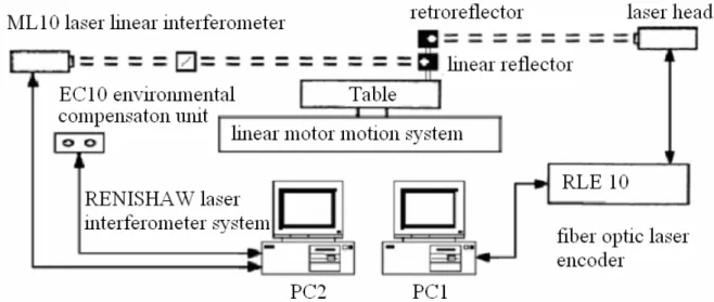
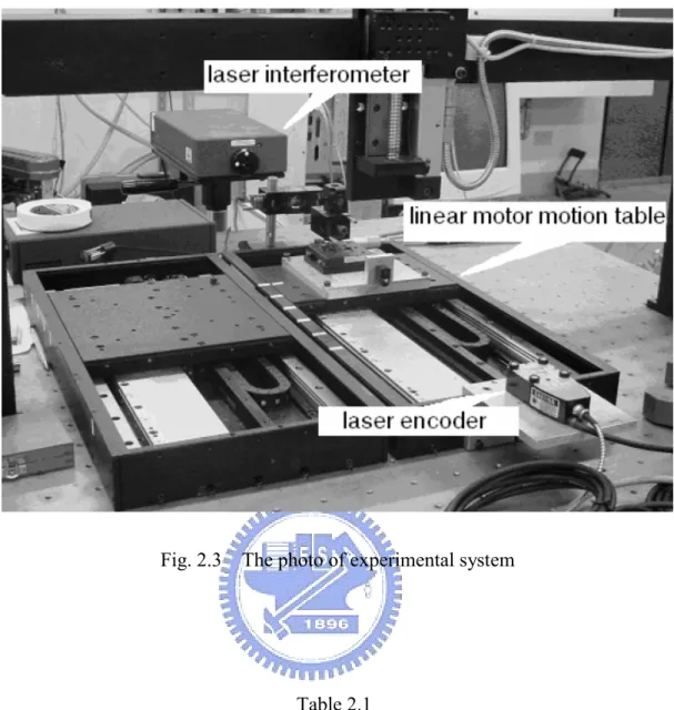
The experimental motion system setup illustrated in Fig. 2.1 consists of following components: a linear-motor-driven motion system, a laser displacement meter, and a PC (PC1 in this figure) with a DAC and encoder interface. The linear motor system is composed of a linear motor (IL6-050A1) and an AC servo amplifier (SERVOSTAR CD) operating in torque (current) mode, both of which are made by Kollmorgen Corporation [88]. Some specifications are listed in Table 2.1. Fig. 2.2 shows the plot of the brushless PM linear motor used in this system. This motor is assembled with 2 linear guide-ways and other mechanical components to form the single-axis motion stage in Fig. 2.3. This mechanism is very simple and with no flexible component between moving slide and guide-ways. There are two sensors used in this system. A linear scale (RENISHAW RGH24Y, resolution 0.1 micrometer)provides position information for the vector control of servo amplifier. A fiber optic laser encoder (RENISHAW RLE10) measures the displacement of the motion table with adjustable resolutions. The fine resolution can reach 20 nm. This high precision for measuring position data enables the high accuracy of velocity estimation and makes the estimation of friction parameters more reliable.

Fig. 2.1 The experimental linear-motor-driven motion system together with the resolution calibration system.

Fig. 2.3 The photo of experimental system

Table 2.1

Some System Specifications of Linear Motor (IL6-050A1)

Specifications Units

Peak force 200 N Peak current 7.0 A Electrical resistance 8.6 Ω Electrical inductance 3.0 mH

Force constant 28.5 N/Arms

2.2 Calibration of fiber optic laser encoder (RLE10)

A high-precision sensor should be applied for data measuring so that the friction behavior could be studied microscopically. In this work, a fiber optic laser encoder is used for measuring position data. The instantaneous velocities are estimated from the high-precision position data by the

αβ

−filter [82].

The accuracy of the resolution supplied by RLE10 depends on some environmental effects, such as relative humidity, temperature, pressure and cosine errors. Therefore, the resolution of this sensor is calibrated by another high-resolution measurement instrument, the RENISHOW laser interferometer system, which includes an environmental compensation unit (EC10). The setup of whole experimental system is shown in Figs. 2.1 and 2.3. Some system specifications of RLE10 are given in Table 2.2. A large displacement, about 200 mm, is used to calibrate the resolution. After calibration, the basic length units (BLU) for course and fine resolutions are found to be 0.020

µ

m and 0.0791

µ

m, respectively. Theoretically, the fine resolution enables us to obtain velocity estimate more accurately. However, the input pulse rate of encoder card used in our system is limited to 1 MHz. We need to adjust the resolution of laser encoder output so that we can perform some experiments in which

Table 2.2

Some System Specifications of RLE10 Fiber Optic Laser Encoder

Axis travel 0 - 4 m

Linearity < ±10nm

Accuracy (uncompensated) 50 ppm

speeds are higher than 20 mm/sec.

2.3 Modeling of the linear-motor-driven system

Fig. 2.4 Cascade control structure of the AC servo system with field-oriented control [89]

The mechanical structure of the linear-motor-driven motion stage is very simple and with no flexible component between moving slide and guide-ways. In Fig. 2.4, the most common structure of a high performance AC servo system is shown. The velocity and position loop controller design will be discussed in Chapter 3. The driving of servo motor is discussed here. By using the field-oriented control, the behavior of AC servo motor is very similar to the DC servo motor [88]. Detailed block diagram of the current controlled power converter is shown in Fig. 2.5. In this diagram, only one of the three phase currents is shown here. The other two phases operate in an identical fashion. Each phase current is controlled by a current regulator to produce the voltage command. The voltage command is compared to a triangle voltage to generate the PWM (pulse-width-modulated) signals that command the power switches to turn-on and turn-off. Then, the inrush current which is provided by the DC bus capacitor flows through these turn-on switches to the motor. The current regulator has a high-gain to minimize the current error over the operating range of the system. The current loop is usually well over 1,000 Hz and the effect of back EMF is eliminated. The electronic dynamics is so fast that the transfer function of AC servo drive can be treated as a constant current gain; therefore, the output force of the motor is equal to K⋅ , where K is a I_T constant and I is the motor current. _T

For simplicity, the high frequency modes that come from both the support mechanical structure of the linear motor and electronic system are ignored. The system equation of the linear-motor-driven stage can be simplified as

u F x B x J _&&+ _&+ ₁= (2.1)

where J is the inertia (equivalent mass); Bx_&+F₁ is the friction force; and u is the input

force to the system generated by a current-controlled servo amplifier. The damping coefficient is considered as a parameter of the controlled plant in this paper, therefore F ₁

represents the friction force without viscous friction term. In general, F is function of ₁

position, velocity and control input force.

Some complex models have been proposed to describe the behavior of pre-sliding friction, such as [26], [62]. However, they are too complicated that identification and implementation of these models are difficult. The LuGre model, proposed by Canudas de Wit et al. [8], can capture most of the known frictional behaviors, and is suitable for control.

In this research, the LuGre model is briefly described, and some notations and variables are defined in next subsection.

2.4 The Dynamic LuGre model

The interface of two contact rigid bodies can be modeled as a lot of elastic bristles. When a tangential force is applied, the bristles will deflect like springs which give rise to friction force. If the force is sufficiently big, some of the bristles deflect so much that they will slip. The LuGre model is based on the average behavior of the bristles and can be described as follows. z v g v v dt dz 0 ) ( σ − = (2.2) dt dz z F₁=σ₀ +σ₁ (2.3)

where z is the average bending displacement of bristles; v is the relative velocity between the two bodies; g(v) is a positive function of velocity; σ₀ and σ₁ are the stiffness and damping coefficient of average behavior of bristles, and F is the friction force due to ₁

bristles’ deflection. A term accounting for the viscous friction could be added to last equation, and the whole friction force becomes

Bv dt dz z

F =σ₀ +σ₁ + (2.4)

where B is the viscous friction coefficient.

The function g(v) can be obtained by measuring the steady state friction when the velocity is held constant. When velocity reaches steady state, friction force is a static map versus velocity. Equations (2.5)-(2.6) show this situation.

Bv v g v Bv z F_ss =σ_{0 ss}+ =sgn( )⋅ ( )+ (2.5) s v v C S C F F e F v g − − + = ( ) ) ( (2.6)

where F_C is the Coulomb (kinetic) friction, F_S is the stick force, and the constant v_s is the Stribeck velocity. The function g(v) used here is a little different from the one taken by Canudas de Wit et al. [8]. It is determined according to experimental data.

2.5 Parameters identification

The detailed procedures for estimating parameters are described in Ref. [94]. The motor inertia J, viscous coefficient B, and Coulomb friction F are first estimated by _C

decoupling the output of DOB estimating method without considering the effect of cogging force. The cogging force exists in the disturbance estimate from DOB; therefore, it does have some influences on the identification. We use the cogging force estimation method in Ref. [94] to improve the accuracy of the parameter estimation. All parameters listed in Table 2.3 will be used in control experiments in following chapters.

Table 2.3

New Identified Parameters of the Experimental System

Symbol and name Value Unit

n

J , inertia 2.49 kg

n

B , viscous friction coefficient 44.14 kg/sec

S

F , static friction force 20.00 N

C

F , Coulomb friction force 5.21 N

s

v , Stribeck velocity 5.0 mm/sec

0

σ , bristle stiffness _1.6484×106 _N/m 1

σ , bristle damping _1.1861×104 _kg/sec

t

K , force constant of motor 28.5 N/A

a

K , gain of current driver 0.349 Volt/A

T, sampling rate 0.0005 sec

p

Chapter 3

Controller Design

In the following, a control structure for a high precision positioning system is proposed. First, a disturbance observer (DOB) is introduces to provide a reliable nominal plant model. Then, minor velocity loop and major position loop are designed based on the nominal plant model. The control structure is based on widely-used cascade control and feedforward control. The bandwidth of the inner control loop, or the velocity loop, is designed to be about 10 times as the outer loop, the position loop. Friction and cogging forces are compensated by the identified models obtained in the previous chapters. Simulations and experiments will follow these design rules developed in this chapter. To find the best structure for future applications, various control structures are compared in simulations as well as in experiments.

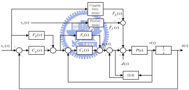
When the DOB, friction, cogging force compensators are added in the proposed feedforward control structure, the whole block diagram looks like the diagram shown in Fig. 3.1 or 3.2. Fig. 3.1 adopts feedback-type compensators while Fig. 3.2 uses feedforward-type compensators. The d(s) appeared in these two figures is the combination of all external disturbances which include the friction and the cogging force. The concept of feedforward (FF) controller design is applied on both the velocity and position loops. This structure is a little different from the FF structure proposed in Ref. [87]. Simulation and experiment will show that the proposed FF structure here is better than the one in the reference paper. Detailed design is described in the following.

3.1 Disturbance observer design

To achieve high precision tracking and position, we must take the uncertainties of system and disturbances into account by the control structure. The model uncertainty, friction, cogging force, exogenous input, etc. are the major resources of system disturbances. In this study, the friction is compensated by the estimated friction via a friction model, and the cogging force is compensated by the additional force estimate via cogging force model. The residual effect and the uncertainties of plant parameters are reduced by the disturbance observer (DOB). In addition, the DOB loop is an inner loop with respect to the velocity loop. Therefore, the DOB loop is designed independently of velocity and position loops. The block diagram of the DOB together with other disturbance compensators are shown in Fig. 3.1 and 3.2, where Fˆ_f andFˆ_g are the estimates of friction and cogging force, respectively.

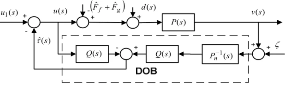
The friction model and cogging force model are obtained in previous two chapters. In these chapters, the DOB is used for identifying parameters of the experimental system; such parameters include the inertia, viscous coefficient and Coulomb friction. But, the estimated disturbance is not used for compensation. In this chapter, the DOB is used for compensating disturbances which come from plant model uncertainty, the residual effects after compensating the cogging force and friction, and other unknown effects. The block diagram of the DOB is shown in Fig. 3.3, where P_n(s)is the nominal plant; Q(s) is a low-pass filter to make sure thatQ(s)P_n−1(s) is proper function and can be realized. Fˆ_f and Fˆ_g are the estimates of friction and cogging force, respectively.

) (s C_p ) (s xr ) (s P ) (s Fv ) (s x s 1 ) (s Fp ) (s Cv ) (s d ) ( 1 s u v(s) ) ( ˆ _s Ff ) ( ˆ s F_g

Fig. 3.1 Block diagram of the proposed feedforward control structure with a disturbance observer and two feedback-type compensators.

) (s Cp ) (s xr ) (s P ) (s Fv ) (s x s 1 ) (s Fp ) (s C_v ) (s d ) ( 1 s u v(s) ) ( ˆ _s Ff ) ( ˆ s Fg ) (s vr

Fig. 3.2 Block diagram of the proposed feedforward control structure with a disturbance observer and two feedforward-type compensators.

) (s P ) (s d ) (s Q _P 1_(s) n− ) (s Q ζ ) (s v ) ( 1 s u u(s) ) ( ˆ s τ

(

Fˆ +f Fˆg

)

Fig. 3.3 Block diagram of the disturbance observer for compensation.

The transfer function of this closed-loop system from u to ₁ v is obtained as follows.

(

( ) ˆ ( ) ˆ ( )

)

( ) ( ) ) ( ) ( ) ( ) ( ₁ 1 s u s G s d s F s F s G s s G s v = _uv + _dv − _f − _g + _ζv ζ (3.1) where ) ( )) ( ) ( ( ) ( ) ( ) ( ) 1 ) ( ) ( )( ( 1 ) ( ) ( ) ( ) ( ) ( )) ( ) ( ( ) ( )) ( 1 )( ( ) ( ) 1 ) ( ) ( )( ( 1 ) ) ( 1 )( ( ) ( ) ( )) ( ) ( ( ) ( ) ( ) ( ) 1 ) ( ) ( )( ( 1 ) ( ) ( 1 s Q s P s P s P s Q s P s P s P s Q s Q s P s P s G s Q s P s P s P s Q s P s P s P s P s Q s Q s P s G s Q s P s P s P s P s P s P s P s Q s P s G n n n n v n n n n dv n n n n v u − + = − + − = − + − = − + − = − + = − + = ζ (3.2)

The estimated disturbance τˆ is fed back to cancel the equivalent disturbance d _e

which includes the uncompensated friction and cogging forces, external disturbances, and parametric uncertainties.

The resulting closed-loop system from the input u to the output v behaves like the ₁

nominal model without the effect of model uncertainties. The equivalent disturbance d is _e

1 ) 1 ) ( ) ( ( ˆ ˆ _u s P s P F F d d n g f e = − − + − ⋅ (3.3)

The last term represents the effect of parametric uncertainties. Let the relationship of system plant P(s)and the nominal model P_n(s) be defined as follows,

) ( ) ( ) (s P s P s P = _n +∆ (3.4)

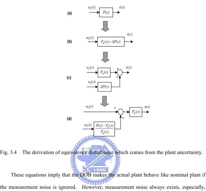
where the ∆P(s) is the model mismatch. The disturbance induced by the plant uncertainty can be obtained from Fig. 3.4 when the other disturbances are ignored. Suppose the model mismatch is large, the corresponding equivalent disturbance will become large. It is possible that actuator saturation happens and causes the instability when the equivalent disturbance is large. Besides, when the nominal model is close to the true plant, the disturbance can be accurately estimated; the minimum control force is therefore obtained. That means the accuracy of identified system parameters is important when minimum control force is under consideration. The method of parameter identification is developed in previous chapters. It can provide accurate parameters for good tracking control.

Since the bandwidth of Q-filter determines the disturbance suppression performance, the DOB design becomes a matter of proper selection of Q-filter. In general, the disturbances are assumed to locate in the low frequency range. Let Q(s)≈1, the three transfer functions in Eq. (3.2) become

1 ) ( 0 ) ( ) ( ) ( 1 − = ≈ ≈ s G s G s P s G v dv n v u ζ (3.5)

) (s P ) (s v ) ( 1s u ) (s v ) ( 1s u ) ( ) (s Ps P_n +∆ ) ( 1s u ) (s P_n ) (s P ∆ ) ( 1s u ) (s v ) ( 1s u ) (s P_n ) ( 1s u ) (s v ) ( ) ( ) ( s P s P s P n n −

Fig. 3.4 The derivation of equivalence disturbance which comes from the plant uncertainty.

These equations imply that the DOB makes the actual plant behave like nominal plant if the measurement noise is ignored. However, measurement noise always exists, especially, in high frequency range. To filter out the high frequency measurement noise, the Q-filter is designed to be Q(s)≈0 in high frequency range. Therefore, the Q-filter used is a low-pass filter with unit DC gain. After applying the DOB, we find that the system plant acts much like the nominal model; hence, we are able to design control law based on the nominal model for the velocity loop.

The DOB can estimate and cancel disturbance. Since the DOB is designed based on linear system theory, it cannot handle discontinuous disturbances very well. For example, large tracking errors will happen due to the discontinuous changes of friction that occur around zero velocity. A sophisticated friction model such as the LuGre model is required to compensate for such discontinuous disturbances.

3.2 Feedforward control

) (s P_n ) (s C ) (s F ) (s X Y(s)

Fig. 3.5 Block diagram of the feedforward structure.

In general, the feedforward control plus feedback controller appears as in Fig. 3.5, where )

(s

P_n is the nominal transfer function of the plant, C(s) is the feedback controller, F(s) is the feedforward controller, X(s) represents the input, and Y(s) represents the response. The transfer function can be expressed as

) ( ) ( 1 ) ( ) ( ) ( ) ( ) ( ) ( s P s C s P s C s P s F s X s Y n n n + + = (3.6)

If 1F(s)P_n(s)= is true, it impliesY(s)= X(s). The system is able to have a response which is rapid and no steady state error. In fact, if F(s)P_n(s)=1 is true, even without the feedback control, i.e., C(s)=0, the system still have good response. However, due to the uncertainty of system and unknown disturbance, the feedback controller is still required to have feedback control loop which can gives a good tracking performance.

3.3 Velocity loop design

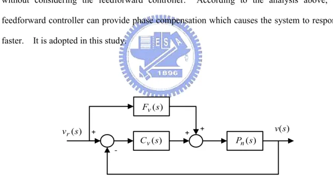
The concept of feedforward control can be applied to the design of velocity loop as well as of position loop. According to concept of the cascade controller design, the velocity loop is designed first. The block diagram of the velocity loop is shown in Fig. 3.6, where

) (s

F_v is the feedforward controller, C_v(s)is the feedback controller, v_r(s)and v(s)are the command input and velocity response respectively. Since the feedforward controller does not change the pole locations of the feedback loop, it does not influence the stability design of the original well-designed feedback system. Therefore, the feedback loop is designed without considering the feedforward controller. According to the analysis above, the feedforward controller can provide phase compensation which causes the system to response faster. It is adopted in this study.

) (s P_n ) (s C_v ) (s F_v ) (s v_r v(s)

Fig. 3.6 Block diagram of the velocity loop.

For the linear motor stage under study, the plant can be expressed as

n n n B s J K s P + = ) ( (3.7)

where the K in this study is equal toK_aK_t; J_n and B_n are nominal values of the inertia and viscous coefficient, respectively. The definition of P_n(s) is different from the definition of previous chapters at that the gain K appears explicitly. This constant gain K

transforms the voltage signal to force unit. From the design concept mentioned above, the feedforward controller can be designed as

K B s J s F_v( )= n + n (3.8)

The above equation is not a proper function and its implementation needs differentiation. In this study, the differentiation is implemented by the digital αβ - filter. This filter performs differentiation in a low frequency range while it decays in high frequency range; therefore, it can provide differentiation with less high-frequency noise. The transfer function of velocity loop becomes

1 ) ( ) ( 1 ) ( ) ( ) ( ) ( ) ( ≅ + + = s P s C s P s C s P s F s L n v n v n v v (3.9)

Since the feedforward controller is not a perfect inverse function ofP_n(s), the velocity feedback controller is needed to eliminate the tracking error. In addition, the regulating control applications and disturbance rejection need good feedback controller for robust performance. Here, the velocity feedback controller is chosen as a PI controller which is defined as follows, s K K s C_v( )= _vp+ vi (3.10)

) (s

C_v can be designed by the pole-placement method. The characteristic equation of ) (s L_v is 0 ) ( 2_{+ + ⋅ + ⋅ =} vi vp n ns B K K s K K J (3.11)

The damping ratio ξ and natural frequency ω_n can be used to represent the characteristic equation as follows, 2 2 2 ( ) ₂ n n n vi n vp n s s J K K s J K K B s + + ⋅ + ⋅ = + ξω +ω (3.12)

The parameters of feedback controller can be obtained by comparing the coefficients of both sides of above equation and are

      = − = K J K K B J K n n vi n n n vp 2 2 ω ξω (3.13)

Since the bandwidth of the current driver is about 800 Hz, the approximated bandwidth of velocity loop ω_n is assigned as 60 Hz or 120π rad/s; and the damping ratioξ is chosen to be 1.

3.4 Position loop design

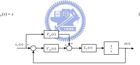
The block diagram of position control loop is shown in Fig. 3.7, where C_p(s)is the feedback controller; F_p(s)is the feedforward controller; X_r(s)and X(s) is the position command and the response, respectively.

According to the feedforward controller design concept, F_p(s)should be the inverse of

s s

L_v( )⋅1. The bandwidth of velocity loop is much larger than the one of the position loop; hence the transfer function L_v(s) can be assumed to be 1. The feedforward controller

) (s F_p is designed as s s F_p( )= (3.14) ) (s C_p ) (s F_p ) (s x_r x(s) s 1 ) (s L_v

Fig. 3.7 Block diagram of the feedforward structure for position loop.

The above equation is not a proper function, therefore, it will be implemented with the digital αβ - filter just like the case in velocity loop design. The position feedback controller is chosen as a P controller in the forward path and is defined as follows,

pp

p s K

where K_ppis the proportional control gain. Then, the transfer function L_p(s) from ) (s x_r to x(s) is obtained 1 1 ) ( ) ( 1 1 ) ( ) ( 1 ) ( ) ( ) ( ≅ ⋅ + ⋅ + ⋅ ⋅ = s s L s C s s L s C s s L s F s L v p v p v p p (3.16)

The parameters of C_p(s) are designed by the pole-placement method. The characteristic equation of L_v(s) is

0 = +K_pp

s (3.17)

The parameters of position feedback controller are obtained by assigning the corner frequency to be ω_n ω_n 12 1 ~ 8 1 , or n n pp K ω ω 12 1 ~ 8 1 = (3.18)

3.5 Comparison of the feedforward structures

The proposed control structure without DOB, friction, and cogging force compensations is shown in Fig. 3.8a, while a referenced structure proposed in [87] is shown in Fig. 3.8b. Let

J J

J = _n+∆ , B=B_n+∆B (3.19)

If the blocks in Fig. 3.8 from Eqs. (3.7-10, 3.14-15) are expanded, the transfer function from )

(s

(

B K K K J

) (

s K K K K K K B

)

s K K K Js Bs Js s X s Y vi pp n pp vp pp vi n pp vp + + + + + + + ∆ + ∆ − =1 _{3 2} 3 2 ) ( ) ( (3.20)

(

B K K

) (

s K K K K K

)

s K K K Js Bs Js s X s Y vi pp vp pp vi vp + + + + + ∆ + ∆ − =1 _{3 2} 3 2 ) ( ) ( (3.21)

The DC gain of these two transfer functions is the same. When the model parameters are accurate, i.e., ∆J =0 and ∆B=0, these two equations have the same value as 1. While

0 ≠

∆J or ∆B≠0, the three poles of Eq. (3.20) and those of Eq. (3.21) will change. The coefficient of s2 term in the characteristic equation of Eq. (3.21) is (B+K_vpK), while that in Eq. (3.20) is (B+K_vpK +K_ppJ_n). The uncertainty of B definitely has greater influence on the change of three pole locations in Eq. (3.21) than in Eq. (3.20). It means that the reference controller design is more sensitive to system uncertainty than to the proposed control structure here.

An experiment is performed to compare the tracking capability of these two feedforward (FF) structures. The position command and the responses, and tracking errors are plotted in Figs. 3.9. Fig. 3.9b shows that the proposed FF control structure is better. Following study will follow this structure and add some compensators.

) (s C_p ) (s F_p ) (s X ) (s P ) (s C_v ) (s F_v ) (s Y s 1 (a) ) (s C_p ) (s F_p ) (s X ) (s P ) (s C_v ) (s F_v ) (s Y s 1 (b)

Fig. 3.8 Block diagrams of two feedforward control structures for the linear motor motion system. (a) The FF structure proposed in this study; (b) the FF structure proposed in reference [87]

0 0.5 1 1.5 2 2.5 3 0 500 1000 1500 pos it ion ( m ic or m et er )

(a) time (sec)

0 0.5 1 1.5 2 2.5 3 -4 -2 0 2 4 6 tr acki n g e rr o r ( m icr o m et er ) (b) time (sec)

Fig. 3.9 Experimental comparison of the proposed feedforward control structure and the one proposed by Ref. [87]. (a) The position command and responses of two different structures. (b) Solid line represents the tracking error of the proposed FF structure, and dash line represent tracking error of the structure proposed in reference paper.

3.6 Simulations of controller design

3.6.1 Test commands

For the examination of the controller performance, two types of desired trajectories are used. A high-order polynomial is used to avoid exciting the high frequency dynamics. This polynomial is defined as Eq. (3.22). The trajectory starts and ends with zero velocity, acceleration. If let A₁=1mm for the displacement and T_r =0.25sec for the transition time, the trajectory can be plotted as in Fig. 3.10.

      > ≤ ≤               +       −       = r r r r r T t A T t T t T t T t A t x , 0 , 10 15 6 ) ( 1 3 4 5 1 1 (3.22)

Furthermore, sinusoidal curves are chosen as trajectories to test the reversals of the direction. The equation is defined as Eq. (3.23). A standard test signal with A₂ =2 mm and

5 . 0 =

p

T sec is plotted in Fig. 3.11.

        − = 1 cos(2 ) 2 ) ( 2 2 p r t A _Tt x π (3.23)

0 0.1 0.2 0.3 0.4 0.5 0.6 0 0.2 0.4 0.6 0.8 1 time (sec) p o si ti o n c o mma n d ( mm)

Fig. 3.10 Trajectory of x_r1 with A₁=1 mm and T_r =0.25sec.

0 0.1 0.2 0.3 0.4 0.5 0.6 0.7 0.8 0.9 1 0 0.2 0.4 0.6 0.8 1 1.2 1.4 1.6 1.8 2 time (sec) pos it ion c o m m an d (m m )

Fig. 3.11 The trajectory of x_r2 with A₂ =2 mm and T_p =0.5s.

The performance comparisons for different controller designs are represented by several performance indices. The first index is the maximum tracking error in the first 0.250 sec is defined as x x E _r t _t = − ≤ ≤ 0.25 0 max max (3.24)

where ”t” represents the transient response region.

To study the accuracy when system reaches steady state, we define the maximum error occurs within the time of 0.25 and 0.6 sec as

x x E _r t _p = − ≤ < 0.6 25 . 0 max max (3.25)

where the small “p” represents the positioning region.

The root mean square error is another commonly used index for performance comparison. Two indices are defined as Eqs. (3.26) and (3.27) corresponding to the transition and positioning regions, respectively.

∑

− = N r rms_t _N x x E 1 ( )2 ,for 0≤ t≤0.25 (3.26)

∑

− = N r rms_p _N x x E 1 ( )2 ,for 0.25< t≤0.6 (3.27) _t

E_max and E_{rms_t} are indices defined for testing the dynamic tracking capability of the control algorithms, while the E_{max_p} and E_{rms_p} are defined for testing the positioning capability.

3.6.2 Control structures

The performance of the control system can be further improved by compensating the friction and cogging forces. The compensator can be divided into two groups which are the feedforward-type compensators and the feedback-type compensators. In the following, eight

control structures are simulated for performance comparison. In this subsection, feedforward-type compensators are implemented. That is to say, they use the reference velocity and position commands as inputs to estimate the friction and cogging forces.

(a) FF: the feedforward control structure only.

(b) FF+CC: the FF control structure plus the cogging force compensator. (c) FF+FC: the FF control structure plus the friction force compensator.

(d) FF+DOB: the FF control structure plus the disturbance observer compensator.

(e) FF+FC+CC: the FF control structure plus the friction and cogging force compensators. (f) FF+DOB+CC: the FF control structure plus the disturbance observer and the cogging

force compensators.

(g) FF+DOB+FC: the FF control structure plus the disturbance observer and the friction force compensators.

(h) FF+DOB+FC+CC: the FF control structure plus the disturbance observer, the friction force, and the cogging force compensators.

For the first step-like test command defined in Fig. 3.10, the tracking errors e1, e2, …, e8, which correspond to the eight different control structures respectively, are plotted in Fig. 3.12.

The performance indices are defined to represent the tracking capabilities of control structures. In Fig. 3.13, they are calculated and plotted according to different definitions. In this figure, the control structure identification numbers (or control id numbers) from 1 to 8 are corresponding to control structures (a) to (h). Figures 3.13a-13d are plotted according to

t

E_{max_} , E_{rms_t}, E_{max_p}, and E_{rms_p}, respectively. Some conclusions can be made from Fig. 3.13.

compensator, cogging force compensator, and disturbance observer.

(2) Although the dynamic tracking capability of the pure FF structure is not as good as the others, the final position of the pure FF structure still can achieve ±20 nm (or 1 BLU). (3) The cogging force compensator has little effect on the tracking accuracy. Because

variation of the cogging force is very small as compared with the reference displacement and velocity. When DOB compensator is added on the control structure, it can detect the slowly varying change of cogging force. Hence, the cogging force compensator can be neglected without affecting the tracking accuracy much.

(4) The nonlinear friction compensation (FC) can improve the dynamic tracking accuracy; however, a larger positioning error is observed. The characteristics of the friction model needs further study when position command no longer changes.

(5) It is very obvious that DOB compensator improves the performance significantly. If the friction and the cogging force compensators are applied at the same time, the performance can further be improved.

(6) The performance of the control structure FF+DOB+FC+CC is almost the same as the performance of FF+FOB+FC. It means that the slowly varying cogging force can be observed by the DOB; therefore, if system has to trade-off a certain compensator to save computation time, the cogging force compensator can be neglected as long as the DOB is applied.

0 0.2 0.4 0.6 -5 0 5 10 15

(a) time (sec)

e1 ( m icr o m e ter ) 0 0.2 0.4 0.6 -5 0 5 10 15 (b) time (sec) e2 ( m icr o m e ter ) 0 0.2 0.4 0.6 -0.2 0 0.2 0.4 0.6 (c) time (sec) e3 ( m icr o m e ter ) 0 0.2 0.4 0.6 -4 -2 0 2 4 (d) time (sec) e4 ( m icr o m e ter ) 0 0.2 0.4 0.6 -0.4 -0.2 0 0.2 0.4

(e) time (sec)

e 5 (m ic ro m e te r) 0 0.2 0.4 0.6 -4 -2 0 2 4 (f) time (sec) e 6 (m ic ro m e te r) 0 0.2 0.4 0.6 -0.4 -0.2 0 0.2 0.4 (g) time (sec) e 7 (m ic ro m e te r) 0 0.2 0.4 0.6 -0.4 -0.2 0 0.2 0.4 (h) time (sec) e 8 (m ic ro m e te r)

Fig. 3.12 The tracking errors of the eight different control structures for the high-order polynomial trajectory defined in Fig. 3.10.

FF FF+CC

FF+FC FF+DOB

FF+FC+CC FF+DOB+CC

1 2 3 4 5 6 7 8 0 2 4 6 8 10 12

(a) structure id number

er ror (mi c rom e ter ) 1 2 3 4 5 6 7 8 0 0.5 1 1.5 2 2.5 3 (b) structure id number er ror (m ic rom e ter) 1 2 3 4 5 6 7 8 0 0.01 0.02 0.03 0.04 0.05 0.06 (c) structure id number e rror ( m ic rom e te r) 1 2 3 4 5 6 7 8 0 0.01 0.02 0.03 0.04 0.05 0.06 (d) structure id number er ror (mi c rom e ter )

Fig. 3.13 The friction and cogging force compensators are implemented in feedforward form. Four performance indices are plotted versus the eight different control structures. The errors (performance indices) are defined as (a) E_{max_t} , (b) E_{rms_t}, (c) E_{max_p} , and (d)

p rms E _{_} . t E_{max_} E_{rms_t} p

E

_{max_}

E

_{rms_ p}

To evaluate the performance of different control algorithms when system encounters velocity reversals, we use the trajectory defined in Fig. 3.11 as the reference command. Fig. 3.14 shows the different tracking errors under the eight different control structures. For the performance comparison purpose, another four indices are defined here.

x x E _r t _s = − ≤ ≤ 0.15 0 max max (3.28) x x E _r t _r = − ≤ ≤ 1.0 15 . 0 max max (3.29)

∑

− = N r rms_s _N x x E 1 ( )2 ,for 0≤ t≤0.15 (3.30)

∑

− = N r rms_r _N x x E 1 ( )2 ,for 0.15< t≤1.0 (3.21)

where “s” represents the starting region, and the “r” represents the reversal regions.

The error when motion start to 0.15 seconds is defined as the error of the control system at the starting region. Eqs. (3.25) and (3.27) are the corresponding performance indices. During the time from 0.15 to 1.0 seconds, there are three motion direction changes, i.e., three velocity reversals happen. Eqs. (3.26) and (3.28) are the corresponding performance indices. They are plotted in Fig. 3.15 with respect to the individual definitions for comparison. From Figs. 3.14 and 3.15, the performance of the FF+DOB+FC and FF+DOB+FC+CC control structures are the best. It is very similar to the previous test that indicates cogging force compensation only has trivial influence on the tracking accuracy.