新興市場通路強度的異質性研究: 中國標竿品牌的市場進入經驗之探討

全文

(1)國立交通大學經營管理研究所博士論文 No.127. 新興市場通路強度的異質性研究: 中國標竿品牌的市場進入經驗之探討 Heterogeneity of Distribution Intensity in Emerging Markets: Exploring Market Entry Experience with Benchmark Brands in China. 研究生：張順全指導教授：唐瓔璋博士中華民國九十八年六月.

(2) 國立交通大學經營管理研究所博士論文 No.127. 新興市場通路強度的異質性研究: 中國標竿品牌的市場進入經驗之探討 Heterogeneity of Distribution Intensity in Emerging Markets: Exploring Market Entry Experience with Benchmark Brands in China. 研究生：張順全研究指導委員會：唐瓔璋. 教授. 丁. 承. 教授. 姜. 齊. 教授. 指導教授：唐瓔璋. 教授. 中華民國九十八年六月.

(3) 新興市場通路強度的異質性研究: 中國標竿品牌的市場進入經驗之探討 Heterogeneity of Distribution Intensity in Emerging Markets: Exploring Market Entry Experience with Benchmark Brands in China 研究生：張順全. Student：Shun-Chuan Chang. 指導教授：唐瓔璋. Advisor：Edwin Tang. 國立交通大學經營管理研究所博士論文. A Dissertation Submitted to Institute of Business and Management College of Management National Chiao Tung University in Partial Fulfillment of the Requirements for the Degree of Doctor of Philosophy in Business and Management June, 2009 Taipei, Taiwan, Republic of China. 中華民國九十八年六月. 3.

(4) 4.

(5) 新興市場通路強度的異質性研究: 中國標竿品牌的市場進入經驗之探討. 指導教授：唐瓔璋. 研究生：張順全國立交通大學經營管理研究所博士班. 摘. 要. 21 世紀伊始，中國經濟成長快速，不但成為全球資訊、通信、暨消費性電子(3C)產業主要生產基地，中國龐大的內需市場，更引起跨國企業覬覦。隨著 2001 年末中國加入 WTO，3C 產業政策更形開放，加上近年來中國政府大力鼓吹「家電下鄉」補貼政策，使得 3C 企業如何深入中國佈局儼然是當前重要的研究議題。然而，中國幅員遼闊，文化複雜性及地域的差異性是廠商在拓展市場時面臨的問題，如何訂定通路強度策略更是各家廠商管理的難題。雖然許多文獻都提及各種影響通路強度的因素，但往往應用已開發市場之研究架構欲解釋中國此一新興市場的通路，則顯扞格不入。本文研究資料涵蓋全中國 200 個城市，包括 2002 年四家 3C 標竿品牌:Nokia 手機、 HP 雷射印表機、聯想電腦及海爾電視機之實際銷售量和中間商鋪點數資料，並連結全國城市各該品類銷售量數據，據以建構各地品牌發展指數（BDI）、品類發展指數（CDI）以及通路強度。作者利用機率模型解析 3C 品牌在中國通路市場佈局的實證經驗，並歸納通路強度的變異除來自可觀測的營銷變數外尚有不可觀測但深具管理意涵的異質性。綜言之，本文研究貢獻整理如下: 1.利用卜瓦松有限混合模型(finite mixture model)和無限混合模型(infinite mixture model) 可將機率分配用來描述通路強度分布的異質性，並由此發展衡量通路市場集中程度的測度; 2.結合品牌發展指數（BDI）、品類發展指數（CDI），探討其與各城市通路強度的關聯性，結果發現和過去在歐美已開發國家的研究所認定運用品牌發展指數（BDI）、品類發展指數（CDI）的市場投資佈局重點順序不同; 3.最後以 NBD 迴歸分析的參數估計結果，表現 3C 標竿品牌在中國通路市場各地佈局變化的意涵，並評估其可能的應用價值。. 關鍵詞：異質性、通路強度、品類發展指數、品牌發展指數、新興市場. i.

(6) Heterogeneity of Distribution Intensity in Emerging Markets: Exploring Market Entry Experience with Benchmark Brands in China. Advisor：Dr. Edwin Tang. Student：Shun-Chuan Chang. Institute of Business and Management National Chiao Tung University. ABSTRACT As most mature markets enter the fray, emerging markets offer an opportunity for global brands to embrace. One of the critical decisions for these firms is how many intermediaries should be used in emerging markets. Although variables affecting market entry and distribution intensity have been proposed by the literature, market background and channel settings context could be drastically different. Factors that account for traditional channel distribution framework in developed markets appear too abrupt to transform go-to-market decision under heterogeneous channel environments for emerging markets. This study empirically examines four benchmark brands, Nokia, HP, Haier, and Lenovo in China’s 3Cs (computer, communication, and consumer electronics) distributors. Our research contributes to a few important fronts for this fast growing and highly competitive market. First, several concentration measures based on the mixture model of Poisson distribution reveal unobserved nature of heterogeneous distribution intensity rates among 200 cities in China. Second, interaction of CDI (category development index) and BDI (brand development index) in representing development of distribution channels is clarified. Third, linking CDI and BDI, the extended Gamma-Poisson mixture regression procedure modeling covariate effects on market growth, distribution capability, and benchmark brands power could be investigated. Results contribute to an applicable mechanism in generating channel intensities among different cities in China.. Keywords: heterogeneity, BDI, CDI, distribution intensity, emerging markets. ii.

(7) Acknowledgements The writing of a dissertation can be an isolating experience, yet it is obviously not possible without emotional and practical support of numerous people. Thus, my sincere gratitude goes to my dissertation advisor, all my family, my parents, and my friends, for their support and patience over the last few years. First, this dissertation would not have been possible without the expert guidance of my esteemed advisor, Professor Tang, Ying-Chan. Not only was he readily available for me, but he always read and respond to the drafts of each chapter of my work more quickly than I could have hoped. Although he is not a man of many words, his oral and written comments are always extremely perceptive, helpful, and appropriate. Many people on the faculty and staff of the Institute of Business and Management at NCTU, assisted and encouraged me in various ways during my course of studies. I am especially grateful to Profs. Mao, Chi-Kuo, Ding, Cherng G.,and Hu, Jin-Li for all that they have taught me. My thanks further go to my family and parents, including my wife Lily, and my two sons, David and Arnold, Dad and Mom, for giving me frequent respite and much love. I also appreciate the welcome and encouragement I have received, in the past decade, from all my kindly colleagues in the Bureau of National Health Insurance, and Department of Health. My enormous debt of gratitude can hardly be repaid to Nicole and some anonymous friends, who not only read multiple versions of all chapters of this dissertation, but also provided many stylistic suggestions and substantive challenges to help me improve my presentation and clarify my arguments. Finally, I wish to thank Dr. Mei-Shu Lai , Dr. Chun-Houh Chen, Dr. Chen-Hsin Chen, Dr. Chao-Yu Guo, and Dr. Wen-Jong Juang, for their inspiring and encouraging me to pursue my Ph.D. degree, so that I felt alone but not lonely in such a long academic journey. Of course, despite all the assistance provided by Prof. Tang and my committee members, I am responsible for the content of the dissertation which may unwittingly remain. -Zachary Zhang. iii.

(8) Contents. 1. Introduction................................................................................................................1 1.1 Background and Research Motivation.............................................................1 1.2 Research Objectives.........................................................................................3 2. Literature Review.......................................................................................................6 2.1 distribution intensity ........................................................................................6 2.2 Concentration and Sunk Cost Investments in Channel....................................7 2.3 Market Concentration Structure and Market Entry Strategy ...........................9 3. Method .....................................................................................................................11 3.1 Finite Mixture Poisson Model of Distribution Intensity................................12 3.2 Gamma-Poisson Mixture Model of Distribution Intensity ............................14 3.3 Concentration Measures Based on NBD Model............................................15 3.4 Application of NBD Regression Model.........................................................18 3.5 The Determined Heterogeneity of Distribution Intensity in Emerging Markets ..............................................................................................................................19 4. Data ..........................................................................................................................23 4.1 Samples ..........................................................................................................23 4.2 Data Description ............................................................................................24 5. Results......................................................................................................................27 5.1 Poisson Model of Channel Density................................................................27 5.2 Gamma-Poisson Mixture Model and Its Applications ................................30 5.3 3C Benchmark Brands’ BDI/CDI Strategies .................................................34 5.4 NBD Regression ............................................................................................43 6. Discussion and Conclusion......................................................................................48 Reference .....................................................................................................................53 Appendix A..................................................................................................................56 Appendix B ..................................................................................................................57. iv.

(9) Contents of Tables TABLE 3.1 CDI/BDI MATRIX…………………………………………………........................... 22 TABLE 4.1 SUMMARY STATISTICS OFDISTRIBUTION INTENSITY ACROSS 200 CITIES IN CHINA..... 25 TABLE 5.1 PARAMETER ESTIMATES AND MODEL SELECTION CRITERIA OF MODELS FOR CHANNEL INTENSITY_ NOKIA…………………………………………………………….……. 28. TABLE 5.2 SUMMARY STATISTICS FOR ECONOMIC INFRASTRUCTURE INDEXES AMONG DIFFERENT DISTRIBUTION INTENSITY CITIES ……………………………..……………….….... 29. TABLE 5.3 THE CONCENTRATION PERFORMANCE MEASURES VARIES MARKEDLY BETWEEN CATEGORIES.………………………………………………………………………... 33. TABLE 5.4 GROUPING CITIES BY THE AVERAGES OF CDI AND BDI…………………………... 36 TABLE 5.5 NUMBERS OF AND AVERAGE DISTRIBUTION INTENSITIES OF CITIES IN EACH GROUP..37 TABLE 5.6 NBD REGRESSION ESTIMATES OF DISTRIBUTION INTENSITY.…………………….….44 TABLE 5.7 NBD REGRESSION ESTIMATES OFDISTRIBUTION INTENSITY IN DIFFERENT CITY-TIER SAMPLES_HP………………………………………………………………….….… 45. v.

(10) Contents of Figures FIGURE 3.1 FLOWCHART OF THE IMPLEMENTATION OF THE TECHNIQUES………………..……. 11 FIGURE 3.2 THE LORENZ CURVE…………………….………………………………………… 16 FIGURE 5.1 FIT OF THE NBD MODEL_DISTRIBUTION INTENSITY…………………………..……31 FIGURE 5.2 3C CDI/BDI SCATTERGRAMS IN CHINA…………………………………………… 35 FIGURE 5.3 CONTOUR PLOT OFDISTRIBUTION INTENSITY- NOKIA (MOBILE PHONE)……….…...38 FIGURE 5.4 CONTOUR PLOT OFDISTRIBUTION INTENSITY- LENOVO (PC)…………….……....…39 FIGURE 5.5 CONTOUR PLOT OFDISTRIBUTION INTENSITY- HP (PRINTER)………….….………...40 FIGURE 5.6 CONTOUR PLOT OFDISTRIBUTION INTENSITY- HAIER (TV)……………..…………. 41. vi.

(11) 1. Introduction 1.1 Background and Research Motivation The commitment to new distribution channel in emerging markets is an adamant investment since it is very difficult to repudiate a distributor even though it is not very productive. From the prolific sides, distribution channel is a strategic asset for a firm that would like to attain sustainable competitive advantages over competitors in strategic matching, such as replicating product designs, underselling on price, and counterfeiting advertising and promotional strategies. Distribution intensity, commonly defined as the number of intermediaries at various distribution channel levels, is the critical element in channel structure to implement these activities (Frazier, Sawhney, and Shervani, 1990; Hardy and Magrath, 1988; Onvisit and Shaw, 1990; Rosenbloom, 1995). In addition, it represents the market outgrowth stake invested by the manufacturer to defend its trading territories (Bonoma and Kosnik, 1990; Corey, Cespedes, and Rangan, 1989; Coughlan, Anderson, Stern, and El-Ansary, 2001; Lassar and Kerr, 1996). Past literature had studied the underlying distribution intensity mechanism and had attempted to explain why firms in similar product category differed in distribution intensity. In their classic works, Frazier and Lassar (1996) proposed several theoretical constructs, such as manufacturer's brand strategy and channel practices, and the moderating effect of retailer requirements that had impacts on distribution intensity. Jain (1993) and Mallen (1996) argued that distribution intensity and the underlying channel structures co-evolved with a host country’s economic developmental stages, while Watson (1997) argued that distribution intensity was the trade-off among customer expectations, company strategy and many other -1-.

(12) uncontrollable factors such as a country's political and legal environment. All these studies investigated the factors that influenced distribution intensity in industrialized markets; not many studies examined these variables in an emerging market context. For emerging markets, such as China and India, the development of economy is unstable. For these potentially largest markets in the world, market structural ambivalence, such as huge trading territories, income inequality, and diversified cultures, abounds in its complicated channel market structure. Distribution of channel intensity is influenced not only by industrial development (Frazier and Lassar, 1996), but also by economic performance (Ingene, 1984; Tang and Li, 1998). Other possible explanation is that some predominant factors might have influence on distribution intensity in this emerging economy. For instance, Li (2003) attempted to identify the determinants of export distribution intensity in emerging markets. His inductive study concerned 18 British manufacturers and their Chinese intermediaries. Five determinants were collected to show a great impact on distribution intensity in emerging markets: behavioral uncertainties, market growth, gray marketing and fake products, distribution capabilities, and transaction-specific investments. Johnson and Tellis (2008) indicated drivers for market entry into China and India are that success is greater with earlier entry, greater control of entry mode, and shorter cultural and economic distances between the home and the host countries, and firms entering more open emerging markets have less success. All the above studies took a deterministic view to investigate distribution intensity. With modeling consideration, even if many researchers attempted to describe/predict distribution intensity using observed determinants, they rely on random components to recognize not all factors were included. Furthermore, since the underlying distribution intensity mechanism might be different in contingent channel settings, it is more difficult to gauge what elements should be involved. -2-.

(13) Krugman (1991) presented an economic geographic framework, showing that the prime impact of most economic activity might be concentrated in one or a few regions. Similar to the existence of heterogeneous economic performance among cities, huge population resides in a few clusters of metropolitan areas in China. Meanwhile, in channel management practice, one critical question marketer may ask is: Should distribution intensity be always concentrated only on a few regions? More interesting research questions are scrutinized toward whether concentration of the distribution intensity patterns on specific sites needs to dispose the same way among different products, and whether few vital parameters could account for distribution intensities.. 1.2 Research Objectives Most high-technology products are introduced in a turbulent, uncertain, and chaotic environmental setting where the odds of success are often low. As a result, the marketing strategies for 3C (computers, communications, and consumer electronics) products must be carefully implemented to enhance the odds of success; yet marketing is often not a well-developed competency for most product-driven high-tech manufacturers. Since the local channel is an indispensable stake for these firms to sell products in a special market, especially the manufacturers in 3C industry rely heavily on channels to transport, stock, distribute, and promote their products. This empirical study subsumes four products (i.e., PC, printer, TV, and mobile phone) to represent 3C category that are widespread in 200 distributed cities in China. The database consists of the number of their intermediaries among 200 distributed cities of four benchmark brands in these categories in 2002, including PC for Lenovo, printer for HP, mobile phone for Nokia, and TV for Haier.. -3-.

(14) The important aspect of this study is to take a new perspective to re-examine the distribution intensity issue in emerging market. In particular, we take into consideration unobserved nature of heterogeneous distribution intensity rates among 200 cities in China by imposing various probability distributions for counting events (Winkelmann, 2008), such as Poisson distribution, Gamma-Poisson mixture distribution (also known as negative binomial distribution, NBD), and Lorenz Curve from NBD (Schmittlein, Cooper, and Morrison, 1993). Since characterizing the right distribution to various channel intensities among cities is more crucial than covariating observed determinants, rashly jumping to import any observed determinant is often exaggerated while the distribution intensity patterns is subtle. This study enumerates three concentration statistics which are closely related to fitting NBD model, such as coefficient of variation, Pareto Shares, and Gini index, to describe prolific sides of the inherent characteristics of distribution channel structures in these cities. To further detect the determinants of distribution intensity in emerging markets on market growth and distribution capabilities from the propositions (Li, 2003). We explicitly add two proxies for these two important constructs to denote different distribution intensity rates among cities. Although applying the dataset in the first year after WTO accession, this study was really completed in the early 2009 during the global recession. The Chinese Central Government suggested the implementation of further measures to propel domestic demand and elicit 3C-proudct consumption with a slogan: “Home appliances going to the countryside”. A government-subsidized project aims to expand sales of household electric appliances in the country's vast rural areas at prices about 13 percent lower than those in cities. This kind of project is not only expected to benefit farmers' living standards but is also expected to help the country's suffering manufacturing sector pull out of the global economic winter. Any further distribution -4-.

(15) channel allocation decisions taken by manufacturers to address the current chances and challenges should also consider not only the specific circumstances of provinces and regions in China, but also the findings mentioned in this study. Transforming market entry strategies for allocated distribution channels from market leader experience as benchmark learning is of paramount importance. In brief, not only is this paper an initially empirical study of 3C benchmark brands experience in China, but also confers the distribution intensity patterns in a generalized manner. This study provides a new perspective of 3C channel structures in China market, the factors that account for the way they are structured, as well as evidence of how investment on channel contributes to devise an applicable mechanism in generating channel intensities among different cities in China.. -5-.

(16) 2. Literature Review 2.1 Distribution intensity Distribution intensity strategy is referred to as the degree to which a manufacturer limits the number of intermediaries, which ranges from a single distributor (exclusive distribution) to an unrestricted number of distributors (intensive distribution) operating within a specific trade area (Fein and Anderson, 1997).distribution intensity has been commonly defined as the number of intermediaries used by a manufacturer within its trade areas (Bonoma and Kosnik, 1990; Corey, Cespedes, and Rangan, 1989; Coughlan, Anderson, Stern, and El-Ansary, 2001). In particular, Frazier and Lassar (1996) defined it as the extent to which a manufacturer relied on numerous retailers in each trade area to carry its brand. To let the product be accessible and available, companies have to decide the ideal number of their intermediaries. Alternatives include exclusive distribution, selective distribution, and intensive distribution (Kotler and Keller, 2009). The traditional channel distribution theory links product class and consumer buying behavior to distribution intensity. That is, different products should use different distribution intensity strategies depending on the characteristics of the product class and consumers appreciate diversity in their consumption. Optimal distribution intensity could supply a suitable amount of products available to target customers without exceeding their needs. In contrast, over-saturated status of distribution intensity would still increase cost, which may be worse than unmet need for lower distribution intensity. In comparison with mature markets, emerging markets may provide global marketers with more attractive market opportunities; yet it will expose global -6-.

(17) marketers to high risks associated with uncertainties (Johansson, 2000). Entry into new environments requires substantial investments, including customer education, distribution channel establishment, and product adaptation (Coughlan, Anderson, Stern, and El-Ansary, 2001). At this point, a large amount of financial investments is required to cover establishment of channel marketing infrastructures and development of market-specific knowledge (Porter, 1990). In other words, investors have to be more careful in emerging markets (Czinkota and Ronkainen, 2001). The fact that China market is growing fast does not mean that investors will be allowed to share the spoils. Li (2003) claimed the propositions in emerging market that the faster the market grew, the more likely that exporting manufactures preferred high distribution intensity. In contrast, the larger the gap is between distributors in terms of distinctive and sustainable capabilities, the more likely it is that exporting manufactures will accept lower distribution intensity. Although Li (2003) also claimed that the more transaction-specific investments are required from distributors, the more likely that exporting manufacturers will accept low channel intensity, we have different approach to these kinds of investments in next section.. 2.2 Concentration and Sunk Cost Investments in Channel Access to distribution channels is often blocked by incumbents in emerging markets that are either first mover or early market entrants (Robertson and Gatignon, 1991). Barriers to entry also make China 3C market environment uncertain for foreign enterprises, and lead to concentrated channel structures that result in reducing competition and raising profits for incumbents. Alternatively, the concept of sunk costs interprets the potential barrier entrants face when entering in an industry if they -7-.

(18) must incur costs that incumbents can somehow avoid (Stigler, 1968). Similar to the advertising being treated as sunk cost (Sutton, 1991) in the US markets; we contend sunk cost theory (Sutton, 1991) could be applied to the supplement explanation of distribution intensity rates among cities. As in Sutton (1991), advertising consists of a fixed and sunk investment. The theory predicts a competitive escalation in advertising levels in larger markets and economics of scale in advertising matter, which limits the extent of entry, and hence bounds the level of concentration away from zero. Sutton (1991) differentiates between endogenous sunk cost (ESC) and exogenous sunk cost. The ESC are costs coming from variables that imply a choice from firms, such as advertising and research and development (R&D), whereas the latter are costs that must be incurred by all entrants, like the sunk costs from scale economies. Using a database spanning 31 industries and the 50 largest US metropolitan markets, Bronnenberg, Dhar and Dube (2005) follow the ESC theory to generate predictions regarding industrial market structure and the roles of brand advertising in consumer package goods (CPG) industries. The evidence predicts that in advertising-intensive CPG categories, market concentration levels should be bounded away from zero irrespective of market size. Industries in which there are endogenous sunk costs (ESC) incurred will have a concentrated structure even if there is a great deal of demand (Sutton, 1991). In Sutton’s (1991; 1998) empirical study, ESC refers to the expenditures undertaken by sellers to improve their products for users, including advertising, R&D, and other brand-enhancing expenditures in consumer goods industries. Expenditures can be considered as ESC only if they meet four assumptions: (1) ESC must be sunk (irreversible); (2) a single firm spending more on ESC raises buyers’ valuation of only that firm’s products; (3) there must be no practical bound to the size of the ESC at any level of expenditures. It is possible to spend more to attract customers; and (4) a large -8-.

(19) fraction of potential customers must respond to the ESC. Sutton argues that in the presence of ESC, markets will only sustain at most a few firms in equilibrium since a firm can invest in ESC to draw many customers to it and accordingly leave other firms to be reduced to secondary market positions. Based on the ESC theory, build-up of a new distributor requires big sunk costs, such as inventory, warehousing, logistics, IT networking, financial capital, HRM, and etc. in order for the new distributor to be productive. In channel market, the market growth will be accompanied by a competitive escalation in distributors’ features, so the number of distributors delivered in the specific cities for some brands may increase dramatically. Investment in 3C channel may constitute an important part as essential as sunk cost for generating brand sales, and thus a probable prediction for brand level is: distribution intensity for different brands could be accompanied by an escalation in distributors’ features as the market grows. In addition, as distribution-intensive brands, their channel market concentration levels should be bounded away from zero.. 2.3 Market Concentration Structure and Market Entry Strategy In economics, market structure describes the competition state of a market, from monopoly to perfect competition. Thus, the main criterion from which one can distinguish between different market structures is to observe the number of manufacturers in the market. In order to have a subtle insight into channel market structures, much more relevant information is not only from the absolute number of manufacturers and their intermediaries within the market, but also from the relative distribution across the markets.. -9-.

(20) Penetration and concentration are more useful criteria to describe relative distribution. A search of the literature about concentration and penetration shows a few articles that have quantitatively addressed in customer purchases (Schmittlein, Cooper, and Morrison, 1993; Anschuetz, 1997; Rungie, Laurent and Habel, 2002). Market penetration typically occurs when a company enters or penetrates a market with current products. On the other hand, market concentration is a function of the number of firms and their respective market shares of the total production (alternatively, total capacity or total reserves) in a market. As strategic implication considered in Schmittlein et al. (1993), the advocators claimed that in low-penetration, low-concentration market, the need to increase awareness and trial is obvious; in low-penetration, high-concentration market, firms must ask if they are purposefully pursuing a niche strategy or approaching a mass market. On the other hand, in high-penetration, low-concentration market, firms may require extensive distribution. Finally, in high-penetration, high-concentration market, firms often battle over the loyalty of the heavy users and market shares. With application to modeling distribution intensity, market entry strategies should be referred to as geographic penetration and channel market concentration as geographic allocation for market dominance made by channel decisions that impact all channel market structure. As far as the penetration of brand levels is concerned, we do not focus on whether the extent of a large portion of the unit sales volume is created by a small portion of channels. On the contrary, we propose that the concentration of distribution intensity involved in a product category is to measure whether. the. magnitude. of. the. high. distribution. distributed-clustering in a small number of specific sites.. - 10 -. intensity. becomes.

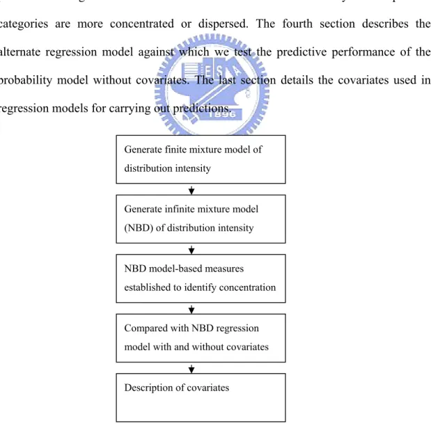
(21) 3. Method In this chapter, we present the method in five sections as shown in Figure 3.1. The first section describes finite mixture model of distribution intensity. The second section shows how the negative binomial distribution (NBD) arises as an infinite mixture of Poisson distributions that represents distribution intensity distributed across the cities. The third section illustrates how the two parameters of negative binomial distribution, the coefficient of variation, Lorenz Curve, Gini index, and Pareto Shares based on the fact that negative binomial distribution can be used to perform the degree of concentration measure and hence identify which product categories are more concentrated or dispersed. The fourth section describes the alternate regression model against which we test the predictive performance of the probability model without covariates. The last section details the covariates used in regression models for carrying out predictions. Generate finite mixture model of distribution intensity. Generate infinite mixture model (NBD) of distribution intensity. NBD model-based measures established to identify concentration. Compared with NBD regression model with and without covariates. Description of covariates. Figure 3.1 Flowchart of the Implementation of the Techniques - 11 -.

(22) 3.1 Finite Mixture Poisson Model of Distribution Intensity At first, we assume distribution intensity is distributed across the cities with an appropriate mechanism responsible for event count data which are distinguished by being positive integer but often with small numbers of unique values. Maximum likelihood techniques based on discrete distributions, such as Poisson distribution, are potentially more efficient in describing the process. Theoretically, the probability modeling of real world data using estimation by maximum likelihood offers a way of tuning the key parameters of the model to provide a good fit (Winkelmann, 2008), and may produce powerful inference on the estimated parameters. These models were originally employed to address the purchase behavior of a population of consumers and used to predict a variety of market statistics such as the distribution of purchase frequencies across households and the average number of purchases per buyer (Schmittlein, Cooper, and Morrison, 1993). With application to utilize these sophisticated statistical tools and to derive estimated parameters from the models, we can use these as explaining convenient descriptors of the unobserved heterogeneity of distribution intensity. Given one product category such as mobile phone, Yi is the number of distribution intensity at city i where consumer can access and purchase this product. Assume Yi is distributed as a Poisson random variable with the same mean λ at all cities. The simple Poisson model is:. P (Yi = y λ ) =. λ y e-λ y!. ,. i = 1, 2,..., 200.. (1). This is a simple Poisson “counting” process which represents exactly Yi number of distributors in city i carry the mobile phone products. It's worth noting that the - 12 -.

(23) Poisson distribution is homogeneous, meaning that every city of the process has the same chance of being selected, which implies that the probability of Yi occurrences in a city depends only on the occurrence counts λ, not on intensity-induced characters such as population size or resident income. We now extend the simple Poisson process to the finite mixture model (FMM) by incorporating the heterogeneity of distribution intensity to the model. The FMM has the ability to distinguish distinct classes of markets, for instance, the cities can be classified by intensity-induced characters such as city tier in metropolitan areas, geographic region, gross domestic products (GDP), population size, retail activity and so on. Although the classification may be adequate for other purposes, it is preferable to classify cities on the basis of resource allocation. Classification of cities into distinguished groups offers a number of advantages over the simple Poisson model.. It provides more accurate predictions for each subgroup. and the stringent market penetration information for 3C–product manufacturers to better gauge potential channel distribution entries. A j-subgroup Poisson mixture arises if j distinct subgroups of channel density can be identified, f (Yi = y ) = P1 f ( y | λ1 ) + P2 f ( y | λ2 ) + ... + Pn f ( y | λn ),. (2). where Yi is number of distributors in city i, Pj is an additive mixture of market penetration level at each subgroup j,. n. ∑ P = 1 , (all Pj > 0, j = 1, . . . , n; j ≤ i ≤200), j =1. j. and the mixing function f ( y | λ j ) is the Poisson distribution with the sub-group mean λj, as defined in equation (1). The j-subgroup Poisson mixture replaces the. - 13 -.

(24) simple Poisson model with a discrete distribution by allowing for multiple (discrete) subgroups each with a different (latent) distribution intensity rate. However, when controlling for the extra parameters, all subgroups can be looked upon as distinct well-defined classes of markets, such as geographic region as mentioned earlier. But they are also n arbitrary subgroups that are freely estimated. Is an n subgroups model better than any other n ± 1 segments model? A common measure for this issue in model building is using Bayesian information criterion (BIC) (Winkelmann, 2008) to compare models fitting and choosing n to minimize BIC.. 3.2 Gamma-Poisson Mixture Model of Distribution Intensity. When modeling distribution intensity data, Poisson model is often the first candidate model. Recall the strong assumption of simple Poisson model, where the number of distribution intensity delivered in each city has a Poisson distribution with equal rate λ. In addition, the FMM allows for multiple (discrete) subgroups each with a different distribution intensity rate. As we move from a finite number of subgroups to an infinite number of subgroups, we propose heterogeneities that across all different cities, i.e., by assuming distribution intensity rate λ has a gamma distribution, a two-parameter family of continuous probability distributions (Winkelmann, 2008). It has a shape parameter α and a scale parameter β shown as follows:. g (λ α , β ) =. β α α −1 − βλ λ e , λ > 0 and α , β > 0. Γ (α ). (3). At the aggregated level, Gamma-Poisson mixture model of distribution intensity is equivalent to negative binomial distribution, NBD (Schmittlein, Cooper, and. - 14 -.

(25) Morrison, 1993). The negative binomial distribution model has the following formula. Γ (.) denotes the gamma function:. Γ (α + y ) ⎛ β ⎞ ⎛ 1 ⎞ f (Yi = y ) = ⎜ ⎟ ⎜ ⎟ , α , β > 0. Γ (α ) y ! ⎝ β + 1 ⎠ ⎝ 1 + β ⎠ α. y. (4). We view the parameters α and β of this distribution as latent characteristics of individual-level channel market at cities. NBD provides useful information, including not only the average distribution intensity across cities, but also the heterogeneity of distribution intensity across cities because of assuming distribution intensity rates from infinite number of subgroups by gamma distribution.. 3.3 Concentration Measures Based on NBD Model. The NBD is defined by two parameters, α and β. As such, we could expect the application to define Pareto Share, as the percentage of total distribution intensity to the top 20% of one brand’s channel markets. The idea of Pareto Share will be linked to Lorenz Curve. Schmittlein, Cooper and Morrison (1993) established (theoretically and empirically) the concentration measure, Lorenz Curve based on NBD. The literature about Lorenz Curve originated from the early years of the twentieth century, Max Otto Lorenz published to outline the technique, which was to bear his name. However, it was the work on poverty and income inequality that led to the popular dissemination and development of the Lorenz Curve and Gini index of income inequality (Gastwirth, 1972).. - 15 -.

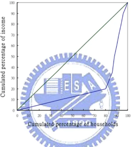
(26) The Lorenz Curve is a graphical representation of the cumulative distribution function of a probability distribution. For example, the prominent evidence shown in Figure 3.2 is called an 80/20 rule or the Pareto Principle (Schmittlein et al., 1993), indicating a certain degree of concentration. The Lorenz Curve is often used to represent income distribution, where the cumulated percentage of households is plotted on the x-axis, while the cumulated percentage of income on the y-axis. In consumer marketing, Pareto Principle also means that the top 20% of a company’s customers have been said to account for 80% of a brand’s sales. 100. Cumulated percentage of income. 90 80 70 60 50 40 30 20 10 0 0. 10. 20. 30. 40. 50. 60. 70. 80. 90. 100. Cumulated percentage of households. Figure 3.2 The Lorenz Curve (Source: Gastwirth, 1972). Since Schmittlein, Cooper, and Morrison (1993) showed that the Lorenz Curve from NBD was based on the unobservable mixing distribution on λ, Gamma distribution g ( λ | α ,β ) in equation (3). It was named “true (long run) Lorenz Curve”, Lλ ( P ) , in their study to show what the true level of concentration was , as opposite to Lorenz Curve calculated from observed numbers. Lλ ( P ) can be calculated as follows:. Lλ ( P ) =. 1. G −1( p ). E ( λ ) ∫0. λ g (λ ) dλ = ∫. β G −1( p ). 0. λα e − λ d λ =G (G −1 ( P | α , 1) | α + 1, 1). Γ(α + 1) - 16 -. (5).

(27) Where. G ( λ | α ,β ). is. Gamma. distribution. C.D.F,. in. equation. (5),. Lλ ( P ) depends only on shape parameter α. The 80/20 type law thus says Lλ ( 0.8 ) =0.2. An interesting observation is exactly how Pareto Share varies with. diverse estimated parameters if Lλ ( P ) =0.2, or P= Lλ −1 ( 0.2 ) , but P is not equal to 0.8. Theoretically, the coefficient of variation (CV) (Schmittlein, Cooper, and Morrison, 1993) of λ is also applied here:. Var ( λ ) E (λ ). α =. α. β2. =. β. 1. α. .. (6). That is, the larger the value of α is, the more homogeneous intensity of channel market in all cities is. By comparison based on observable number of distribution intensity, we can also calculate the “empirical” coefficient of variation as follows:. Var ( y ) E ( y). =. α⋅. 1 ⋅ (1 + β ) β 1+ β 1+ β = . α /β α. (7). It is worth noting that “empirical” coefficient of variation varies with more than simply the α parameter. We find out that observed concentration level among different products will be increased as β grows. In addition, we will focus on the measure of Gini index based on Lorenz Curve with the unobservable mixing distribution on λ, which is calculated from its original. - 17 -.

(28) geometry definition and numerically approximated by Simpson's rule (Atkinson, 1989) as follows: 1. 1− 2∫ Lλ ( P) dP .. (8). 0. In summary, the Gini index is so sufficiently simple that it can be compared across product categories and be easily interpreted as overall concentration measure, but the Lorenz Curves can have different shapes and yet still yield the same Gini index. In other words, the Gini index is more intuitive to many people since it is based on the Lorenz Curve. However, it is not easily decomposable. In contrast, Pareto Share based on the Lorenz Curve indicates how important the top 20% of one brand’s channel markets is. Otherwise, the advantage of reporting CV can also be used to represent the concentration of different products concisely to compare other measures. These are the reasons we use different concentration measures in this study that may gain more special insight into how the concentration effect varies with such informative and systematic indicators, and find out the key parameter, α in NBD model, which is proportional to the degree of homogeneity among these indicators.. 3.4 Application of NBD Regression Model. In negative binomial distribution, NBD model, we assume Yi is distributed as a Poisson random variable with mean λi. Furthermore, we suppose each individual’s mean λi is related to their observed explanatory characteristics. That is, via regression modeling, we can add deterministic heterogeneity to NBD model. The regression model would be of great benefit in improving fit over simple probability model. - 18 -.

(29) without covariates, and in testing determinants influencing distribution intensity. The negative binomial regression model arises if this heterogeneity is modeled using the gamma probability distribution. The density of the negative binomial is derived by adding an error term to the conditional mean of the Poisson distribution (Cameron, and Trivedi, 1998):. /. λi = e γ xi + ε. or. (9). ln(λ ) = γ xi + ε, /. where exp(ε) follows a gamma distribution with mean one and variance 1/α. Substituting Equation (9) into Equation (3), and integrating ε out of the expression yields the density. Γ (α + y ) ⎛ ⎞ ⎛ e γ ′xi ⎞ β P (Yi = y ) = ⎟ , ⎜ ⎟ ⎜ Γ (α ) y ! ⎝ β + e γ ′ x i ⎠ ⎝ β + e γ ′ x i ⎠ α. y. (10). where the density reduces to original NBD model when γ =0, showing no determinants influencing distribution intensity.. 3.5 The Determined Heterogeneity of Distribution Intensity in Emerging Markets. As an emerging market grow fast, the volume and the frequency of transactions through the channels will be increased. Consequently, companies have to resort to high distribution intensity to suppress channel conflicts and reduce dependence on individual distributors. In this research, the main criterion by which one can represent market growth is category development index (CDI), being referred to as fair share - 19 -.

(30) index. CDI is an efficient tool used to measure market development of a specific product category in specific region. It could be calculated by a market’s category sales percentage divided by the total population percentage of that market.. CDI =. Percentage of product catgory total sales in market Percentage of total population in market. (11). CDI is commonly used in category management to measure the performance of category sales of retailers (Dhar, Hoch, and Kumar, 2001), but it can also be used to evaluate market size of a category in a particular geographic area. Companies can use CDI to understand development situation in a specific market compared to all markets in order to help make go-to-market decisions. On the contrary, manufacturers usually do not accept exclusive agency unless distributors are exceptionally brilliant. Li (2003) stated that some of the manufacturers indicated that the appointment of exclusive agent would be detrimental to their market coverage but they had to accept it. In this study, like CDI for category, brand development index (BDI) is the counterpart index for a particular brand. BDI, which helps marketers make decisions, is calculated by a market’s brand sales percentage divided by the total population percentage of that market:. BDI =. Percentage of brand to total sales in market Percentage of total population in market. (12). The BDI can determine the sales potential for a brand in a specific market area. The higher the index is, the more market potential it should be. The BDI can also help marketers to understand their current product’s performance and penetration situation to deal with brand management. Given one city, we have the real data of sales volume - 20 -.

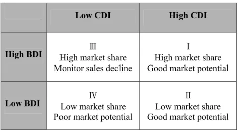
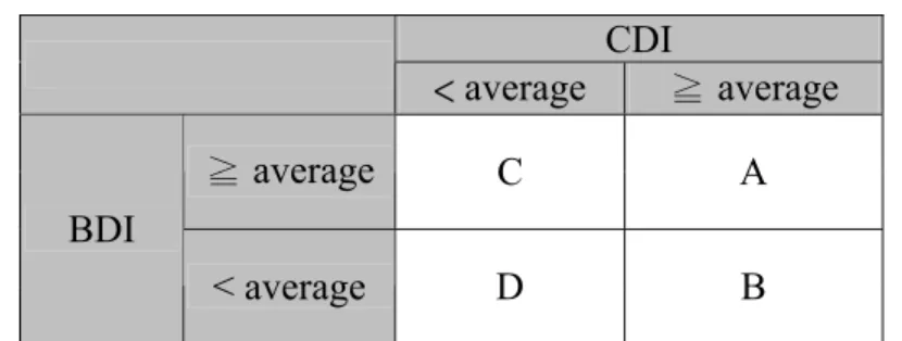
(31) the local Chinese intermediaries can generate. However, some resellers are large, and others might be small. In other words, different scale of intermediaries in the city might generate different sales. Li (2003) identified one possible negative determinant on distribution intensity in emerging markets, distribution capabilities, as a major influential covariate. Therefore, by devising the BDI divided by the number of intermediaries, we can define such measure representing the actual performance of local channels, that is, distribution capabilities. CDI and BDI can describe market entry strategies with a 2 x 2 matrix, which separates the markets (Belch and Belch, 2004) as shown in Table 3.1.These various segments have different market potential. The market with high CDI and BDI (Ⅰ) represents good sales potential for both the product category and the brand itself. Otherwise, the one with high CDI but low BDI (Ⅱ) shows that customers appreciate this product category but are not willing to purchase the specific brand. While a market has low CDI but high BDI. (Ⅲ), the sales amount of the brand is performing. better than that of the other categories. That is, the customers seem to like the brand even if it is just a burgeoning product category within the market. Besides, the market with low both CDI and BDI (Ⅳ) represents that neither the product category nor the brand has been performing well. It is not a good target market for further investment, such as advertisements, inventory, logistics, IT networking, financial capital, HRM, and etc.. - 21 -.

(32) Table 3.1 CDI/BDI matrix Low CDI. High CDI. High BDI. Ⅲ High market share Monitor sales decline. Ⅰ High market share Good market potential. Low BDI. Ⅳ Low market share Poor market potential. Ⅱ Low market share Good market potential. Source: (Belch and Belch, 2004). - 22 -.

(33) 4. Data This chapter details our data sources, procedure for data collection, and data description.. 4.1 Samples Quer et al. (2007) reviewed the empirical articles focusing on the Chinese context published in 12 leading international academic journals between 2000 and 2005. Regarding the methodology applied, the quantitative approach was used in 148 of the 180 studies (82.2%). They also argued that due to the restrictions imposed by the Chinese authorities on the collection of information, foreign researchers frequently had to seek the support of the National Bureau of Statistics of China, or of Chinese enterprises specialized in market research. Correspondingly, as for the quantitative papers, which utilized reliable information, the primary data source in our research collected by a Chinese leading 3C distributor specialized in 3C channel market research, consists of four leading brands in different product categories within 3C industry in 2002, including PC for Lenovo, printer for HP, mobile phone for Nokia, and TV for Haier. These four product categories are generally classified as 3C products, but, in fact, they all have different characteristics and belong to various product life cycles. Two out of these companies are foreign companies, HP and Nokia, and the other two, Lenovo and Haier, are local enterprises and the flagship Chinese brands. The number of intermediaries, product category sales in volume units, and brand sales in volume units of these brands in 200 cities in China are included in this database. These cities (shown in Appendix A) are not chosen randomly but chosen by - 23 -.

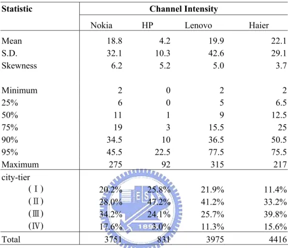
(34) city-tier so that the first-tier cities would be selected first, and then, the second-tier ones would be included successively. As a result, the two hundred cities in the database are relatively representative among all of the cities in China. Another auxiliary database used is China City Statistical Yearbook published by China Statistical Publishing House. It indicates economic infrastructure data among these cities.. 4.2 Data Description. This dataset identifies four categories of 3C industry in China, i.e., PC, printer, TV, and mobile phone. The leading brands are, Lenovo, HP, Haier, and Nokia, respectively. Table 4.1 reports summary statistics of the distribution of distribution intensity for these four leading brands. Since many PC owners did not buy any printer in the emerging market, China PC penetration rate was low at that time, not to mention the printer. Except for HP, the total number and the average of distribution intensity in different brands are similar. However, a great deal of variability can be observed by standard deviation divided by mean in Table 4.1, and the data are very positive skew as we can see that distribution intensity is soaring from 95 percentile to maximum intensity. In a skewed distribution, the mean is farther out in the long right tail than the median. The skewness shows that its distribution is not symmetric like the bell-shaped normal curve, especially in Nokia and HP (Skewness=6.2 and 5.2, respectively). In both Chinese brands, the distribution intensity of Lenovo averages slightly less than that of Haier, but the variation in distribution intensity of Lenovo is larger.. - 24 -.

(35) Table 4.1 Summary statistics of distribution intensity across 200 cities in China Statistic. Channel Intensity Nokia. HP. Lenovo. Haier. Mean S.D. Skewness. 18.8 32.1 6.2. 4.2 10.3 5.2. 19.9 42.6 5.0. 22.1 29.1 3.7. Minimum 25% 50% 75% 90% 95% Maximum city-tier (Ⅰ) (Ⅱ) (Ⅲ) (Ⅳ). 2 6 11 19 34.5 45.5 275. 0 0 1 3 10 22.5 92. 2 5 9 15.5 36.5 77.5 315. 2 6.5 12.5 25 50.5 75.5 217. 20.2% 28.0% 34.2% 17.6% 3751. 25.8% 47.2% 24.1% 3.0% 831. 21.9% 41.2% 25.7% 11.3% 3975. 11.4% 33.2% 39.8% 15.6% 4416. Total. Table 4.1 also provides summary statistics for the city-tier classification used in this analysis. If the market visibility of a product category is high, we expect the number of its distributors should also be high. As shown in Table 4.1, the most common resource (distributors) allocation is setting in city-tier (Ⅱ), and city-tier (Ⅲ), followed by city-tier (Ⅰ) where only three metro cities, ShangHai, Beijing, and GuangZhou make up of the samples. The complementary effect also reveals different companies’ strategies. As the printer is complementary to the PC, i.e., we assume the consumer who owns a printer must also own a PC. This is one reason we can observe the similar distribution intensity patterns by city-tier both in HP and Lenovo among larger cities (city-tier - 25 -.

(36) (Ⅰ), (Ⅱ), and (Ⅲ)). Moreover, because of low penetration rate of the printer at that time, HP had cautiously selected its resellers. As shown in Table 4.1 , HP’s decision did not focus on city-tier (Ⅳ). The result by city-tier classification is reasonable (i.e., printer penetration rate is less than PC penetration rate in small market potential cities, not to mention market penetration of TV or mobile phone), while HP’s distribution intensity in city-tier (Ⅳ) is also less than that of any other brand in the dataset.. - 26 -.

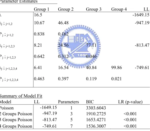
(37) 5. Results We present the results on finite mixture model from Poisson distribution, infinite mixture model (NBD) and its applications, BDI/CDI strategies, and NBD regression model.. 5.1 Poisson Model of Channel Density Table 5.1 provides the parameter estimates and model selection criteria of the Poisson model in equation (1) and (2) in analyzing distribution intensity of one benchmark brand such as Nokia. If two distinct segments, heavy and light intensities, are assumed, both BIC (Bayesian information criterion) and common likelihood ratio (LR) test (Winkelmann, 2008) reject the null hypothesis that channel densities of heavy and light segments are equally distributed since two segments model yields smaller BIC (=1910.3 < 3303.6043) and LR (= 2*|1649.15-947.19|) > Χ2 0.05, 2. The associated channel intensities λ 1 and λ 2 are 10.67 and 46.48, while the city penetration rates are 83.8% and 16.2%, respectively. The result indicates that Nokia products are unequally distributed to two distinct segments. The distribution intensity can be analyzed stepwisely to four distinct segments, where p-value of LR is less than 0.001 to show four segments model fits the data better than three segments model. Four segments model also has smallest Bayesian information criterion (BIC) in our analysis. The associated channel intensities λ1,λ2, λ3, and λ4 are 6.41, 16.54, 40.84, and 99.86, while the market-penetration levels are 46.3%, 39.7%, 11.9%, and 2.1%, respectively. That is, group 1 shares 46.3% of Nokia’s channel distribution and group. - 27 -.

(38) 2 shares 39.7%, and vice versa. The fact that higher lambda value yields low market-penetration level is due to the nature of Poisson distribution on distribution density where the occurrence of distributed channel’s probability is low, but the number of opportunities for occurrence is high – both groups 3 and 4 have high distribution intensity, despite their relatively small shares.. Table 5.1. Parameter estimates and model selection criteria of models for distribution intensity_ Nokia. Parameter Estimates Group 2. λ. Group 1 16.5. Group 3. Group 4. λj ; j=1,2. 10.67. 46.48. P j ; j=1,2. 0.838. 0.162. λj ; j=1,2,3. 8.21. 24.56. 77.11. P j ; j=1,2,3. 0.642. 0.312. 0.046. λj ; j=1,2,3,4. 6.41. 16.54. 40.84. 99.86. P j ; j=1,2,3,4. 0.463. 0.397. 0.119. 0.021. LL -1649.15 -947.19. Summary of Model Fit Model LL Parameters -1649.15 Poisson 1 -947.19 2 Groups Poisson 3 3 Groups Poisson -813.47 5 4 Groups Poisson -749.61 7. BIC 3303.6043 1910.2725 1653.4271 1536.3007. -813.47. -749.61. LR (p-value) <0.001 <0.001 <0.001. Although the four groups are separately identified due to their different channel densities, there are some limitations for the application use of Poisson distribution model since the outliers (extremely low or extremely high) of actual distribution intensity might not be able to detect. In other words, among Nokia’s 275 channel - 28 -.

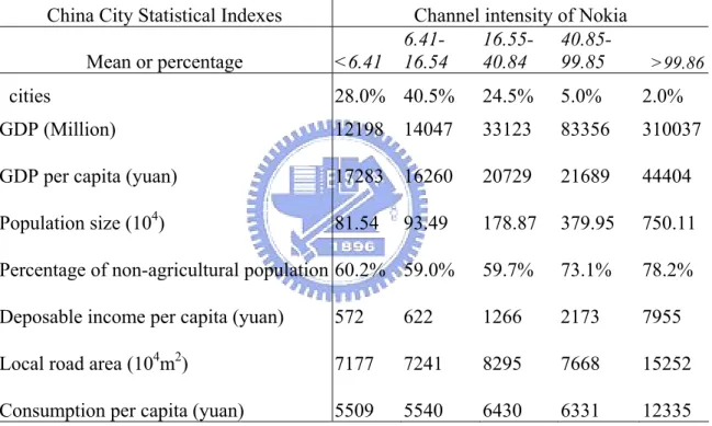
(39) density maximum, some types of counts of channel density smaller than 6.41 or channel density greater than 99.86 may fail to generate the proper occurrence. Since four cutoff pints have been indentified, we now use economic and infrastructure indicators that include GDP per capita, gross domestic products (GDP), and population size to identify those summary statistics for economic performance of different cities as shown in Table 5.2. Table 5.2. Summary descriptive statistics for economic infrastructure indexes among different distribution intensity cities. China City Statistical Indexes Mean or percentage cities. <6.41. Channel intensity of Nokia 6.4116.55- 40.8516.54 40.84 99.85. >99.86. 28.0% 40.5%. 24.5%. 5.0%. 2.0%. GDP (Million). 12198. 14047. 33123. 83356. 310037. GDP per capita (yuan). 17283. 16260. 20729. 21689. 44404. Population size (104). 81.54. 93.49. 178.87. 379.95. 750.11. Percentage of non-agricultural population 60.2% 59.0%. 59.7%. 73.1%. 78.2%. Deposable income per capita (yuan). 572. 622. 1266. 2173. 7955. Local road area (104m2). 7177. 7241. 8295. 7668. 15252. Consumption per capita (yuan). 5509. 5540. 6430. 6331. 12335. As we can see from those cities with higher distribution intensity in the Table 5.2, the values of economic infrastructure indexes are also higher. The top 2% cities command the highest GDP (RMB$310,037 million), population size (7.5×106), disposal income and consumption expenditure. The monotonically increasing relationship between distribution intensity and economic infrastructure indicator reveals that Nokia prefers to develop higher channel density in higher economic growth areas. This evidence could provide an example to show that the faster the - 29 -.

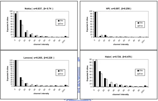
(40) market grows, the more likely that exporting manufactures prefer high distribution intensity.. 5.2 Gamma-Poisson Mixture Model and Its Applications The Poisson distribution of channel density results come with some limitations including the process is assumed to have a certain rate of regularity among segments and the inability to model underdispersed counts for extreme low and extreme high cases. The hierarchical Poisson model with Gamma prior, so called the NBD (Negative Binomial Distribution) model in equation (4), allows capturing latent propensity for channel distribution for each particular city in each product category. We use infinite mixture of Gamma-Poisson distribution in this section where the Gamma distribution represents different channel intensity distributed across the cities rather than FMM. The Gamma distribution retains two parameters α (the shape parameter) and β (the scale parameter) to accommodate the heterogeneity of channel density across cities. The shape parameter is directly proportional to the latent propensity for channel distribution; the larger the value of α, the more homogeneous intensity of channel market in all cities for each product category. The scale parameter controls the balance of heavy and light channel density within each product category, if scale parameter increases, the proportion in heavy channel density is higher. Concentration of channel density regarding NBD model has been discussed in section 3.3. While modeling NBD approach to each channel intensity data, we derive estimated NBD parameters to report statistics for the distribution of channel intensity in each 3C category. In Figure 5.1, the fitting of the distribution is a matter of determining which two parameters create the shape and scale of the NBD that most - 30 -.

(41) closely fits the observed data. The observed and theoretically expected distributions for each category are plotted on the same set of axes in order to give a picture of these 3C benchmarks’ channel structures. While looking at histograms of channel intensity, distribution is valuable for considering the fit of the model and gaining a “picture” of the channel allocation behavior.. 80. 70. 60. 50. 40. 30. 20. 0. Haier( α=0.724, β=0.478 ) 90. Expected # cities. 80. Obs Exp. 70 60 Obs. 50. Exp. 40 30 20 10. channel intensity. 10 0+. 90. 80. 70. 60. 50. 40. 30. 20. 0. 10. 90. 10 0+. channel intensity. 80. 70. 60. 50. 40. 30. 20. 10. 0 0. Expected # cities. Exp. channel intensity. Lenovo( α=0.265, β=0.228 ) 120 110 100 90 80 70 60 50 40 30 20 10 0. Obs. 90 10 0+. channel intensity. 90 10 0+. 80. 70. 60. 50. 40. 30. 20. 10. Exp. 100 90 80 70 60 50 40 30 20 10 0 10. Expected # cities. HP( α=0.097, β=0.256 ). Obs. 0. Expected # cities. Nokia ( α=0.837, β= 0.74 ) 100 90 80 70 60 50 40 30 20 10 0. Figure 5.1 Fit of the NBD model_ distribution intensity. In Figure 5.1, the first thing we see is that light bars and dark bars denote closely with each other to show goodness-of-fit. By further calculation of the differences between light bars and dark bars in each part of Figure 5.1, aside from the best fit of the NBD distribution model in Haier (p-value of Chi-Square Goodness-of-Fit Test = 0.76), the least fit of the NBD distribution model in Lenovo is also reliable (p-value of Chi-Square Goodness-of-Fit Test = 0.09). We also calculate that approximate numbers of channel intensity in more or less than 100 are not over 10 cities, and that only small parts of cities are over 30, especially for HP.. - 31 -.

(42) These four channel intensity distribution figures exhibit the classic reverse J-curve of the NBD for certain parameter values. We can imagine that the NBD draws a line straight through the histogram and describes the 3C leaders’ channel allocation behavior. It is valuable to note whether the “tail” to the right hand side of the graph is fatter. We will later show that the fatter “tail” of the cities with higher channel intensity gives a higher Pareto Share. As a whole, the infinite mixture model (NBD) is able to fit these types of 3C leaders’ channel intensity instead of finite mixture Poisson model. In reality, categories have big and small markets in China. In the empirical study of this phenomenon, we examined four categories of 3C products data in 2002, and asked the key question, “How important to marketing strategy is the top concentration 20th percentile of the market base?”. The NBD’s two parameters, α and β, coefficient of variation in equation (6) and (7) tells the scale and shape of channel density;. the. Gini index based on equation (8) captures the degree of concentration of that density, the theoretical Pareto Shares based on equation (5), and the observed Pareto Shares as the percentage of total channel intensity to the top 20% of one brand’s channel markets, considers how resources are distributed among cities and define the pareto-optimality of channel density. Compared with equation (6), the “empirical” coefficient of variation (7) based on observable number is proposed to decrease with the increases of category’s homogeneity (α) and to change according to that category’s scale (β) parameter. An increase in β represents an increase in the coefficient of variation in equation (7). On the other hand, Pareto Share is calculated from the percentage of the total brand channel intensity accounted for by the top 20th percentile of its channel markets. Theoretical values of Pareto Share are calculated from the theoretical (NBD) estimates in equation (5) that we have adopted each α in Figure 5.1. Schmittlein, - 32 -.

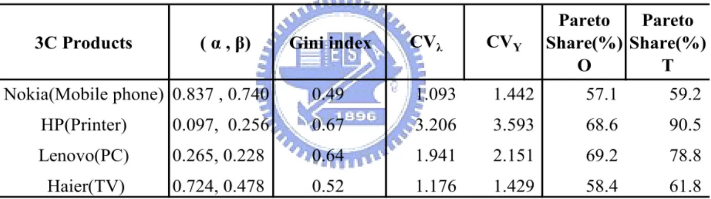
(43) Cooper, and Morrison (1993) demonstrated that the NBD could be extrapolated to estimate the market behavior for periods beyond the observed period in consumption data. We assess the theoretical Pareto Share in NBD for the same purpose to extrapolate into longer time period since we have only one-year cross sectional data. In order for transforming go-to-market strategies from the inference in NBD model-based analysis, the theoretical concentration statistics based on latent market concentration structure can provide insight into a company’s long-range planning for resource allocation. Since companies establish new distribution channel in emerging markets is an adamant investment, one-year observed measures may mislead decision.. Table 5.3 The concentration performance measures varies markedly between categories 3C Products. ( α , β). Gini index. Nokia(Mobile phone) 0.837 , 0.740. CVλ. CVY. Pareto Pareto Share(%) Share(%) T O. 0.49. 1.093. 1.442. 57.1. 59.2. HP(Printer). 0.097, 0.256. 0.67. 3.206. 3.593. 68.6. 90.5. Lenovo(PC). 0.265, 0.228. 0.64. 1.941. 2.151. 69.2. 78.8. Haier(TV). 0.724, 0.478. 0.52. 1.176. 1.429. 58.4. 61.8. 1.CVλ: the coefficient of variation based on unobservable or latent concentration structure. 2.CVY: the coefficient of variation based on observable number. 3.Pareto Share ( O= observed, T = theoretical).. Table 5.3 illustrates the consistency in relative concentration levels and sales productivity of distribution intensity among different 3C leaders. For empirical coefficient of variation in channel intensity distribution, only HP is greater than 3, says that HP established its most of channels just in small portion of cities. The CV value (3.593) was above Lenovo (2.15), Nokia (1.44) and Haier (1.42), infers that printer was less appeal than Mobile phone or TV among cities in China at that time. The observed Pareto Share (0.686) for HP was also greater than those of Nokia (0.571) - 33 -.

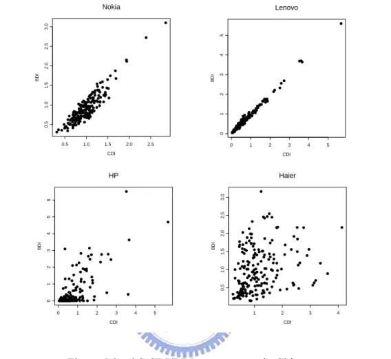
(44) and Haier (0.584), meaning that HP’s top percentile of market base was much more than those of Nokia or Haier. As a result, the theoretical Pareto Share for the two categories, printer for HP (.905), and PC for Lenovo (.788) accounted for more than 78%, which is “high channel intensity.” Both HP and Lenovo follow faithful the Pareto principle to allocate nearly 80% of their channel density in 20% of the cities. For the other two market leaders, Nokia (0.49) and Haier’s (0.52), their Gini indexes were low, meaning both companies widespread their distributions to more cities. All these measures above reflect concentration of resource allocation. In particular, the parameter α demonstrates a good concentration performance measures to deal with channel market bases, while the Pareto Share can add depth to the analysis of channel concentration.. 5.3 3C Benchmark Brands’ BDI/CDI Strategies In this section, many interesting patterns will be geared down with application to BDI and CDI. For instance, BDI/CDI calculates the visibility (distribution efficiency) of a brand. If the ratio is high, we expect the number of distributors should also be high. The logic is that if the BDI is high, then the firm has put many efforts to the city. Therefore, if the ratio is greater than one (i.e., BDI > CDI), then the company might waste some resource to distribute to that city. The reason why a company makes such decision might be due to the intensive competition, or, the expectation of the future growth potential of that city, and vice versa. The upper part of Figure 5.2 shows that Nokia’s and Lenovo’s CDI vs. BDI distribution patterns among 200 cities. The x-axis is for CDI, and BDI is on the y-axis. The upper half of scatter plots obviously. - 34 -.

(45) indicates that distribution pattern nearly follows a straight line. It means that the more CDI number is, the more BDI will be. Nokia. 3 0. 0.5. 1. 1.0. 2. 1.5. BDI. BDI. 2.0. 4. 2.5. 5. 3.0. Lenovo. 0.5. 1.0. 1.5. 2.0. 2.5. 0. 1. 2. CDI. 4. 5. Haier. BDI. 3 0. 0.5. 1. 1.0. 2. 1.5. 4. 2.0. 5. 2.5. 6. 3.0. HP. BDI. 3 CDI. 0. Figure 4.3 3C CDI/BDI scattergrams in China 1. 2. 3. 4. 5. 1. CDI. 2. 3. 4. CDI. Figure 5.2 3C CDI/BDI scattergrams in China. Lenovo’s market entry pattern is similar to Nokia’s, the ratio of BDI/CDI is close to one. As a contrast to Nokia’s scatter plot, Lenovo’s pattern is much relatively closed along the 45 degree line, indicating that market entry pattern for Lenovo is “to dance to the other PC companies’ tune” and thus close to the path of total development of PC products in the markets. Lenovo has aggressively distributed its products; therefore, the resource (distributors) allocation does not seem to be efficient, i.e., it has distributed many small (market potential) cities where both CDI <1 and BDI< 1.. - 35 -.

(46) Although the governmental data does not include the printer data, printer is complementary to the PC, i.e., we assume the consumer who owns a printer must also own a PC. Therefore, we calculate CDI for PC to represent CDI for Printer, called PC_CDI. The result is reasonable (i.e., printer penetration rate is less than PC penetration rate) since many PC owners do not buy printers. Because of low penetration rate of the product, HP has cautiously selected its resellers. As a result, HP’s decision is more fit with Westerner’s thinking, i.e., it focuses on the cities where BDI >1 and PC_CDI > 1. Figure 5.2 also shows HP’s distribution pattern, which is totally different from the patterns in upper part of Figure 5.2. The pattern of HP’s market development seems to have a random shape, but most points of the cities are distributed as BDI and PC_CDI are greater than one. The lower half of Figure 5.2 also illustrates Haier’s pattern. Distinct pattern from other companies, Haier’s channel market penetration pattern is not followed by another Chinese brand, Lenovo. It is filled with “full coverage market” consideration. Although these market leaders’ products are all categorized into 3C products, their market penetration strategies seem to be quite different. If we want to explore their difference among 200 cities in China, we can divide these cities into four city groups, A, B, C, and D, according to CDI and BDI. In this study, we use the averages of CDI and BDI as the operational definition of threshold to divide the markets to match the classification in Table 3.1, and it is shown in Table 5.4.. Table 5.4 Grouping cities by the averages of CDI and BDI CDI < average ≧ average ≧ average. C. A. < average. D. B. BDI. - 36 -.

(47) The number of cities in four different market groups for each brand is shown in Table 5.5. Except for Nokia, the market development situation of the other three companies, Haier, Lenovo and HP, are rather similar in the group D. The group D has most numbers of cities across these three brands, especially for Lenovo, as Table 5.5 shows that more than half of the 200 cities belong to group D. Using average distribution intensities among city groups as market penetration ratio, we also use city group at four brands as another classification for dataset. The further analysis of the Chi-Square test shows that inconsistent patterns under these two classifications (p-value < 0.01). That is, the distributions of channel allocation in these four products look like following different market penetration ratios.. Table 5.5 Numbers of cities and average distribution intensities of cities in each group. (Numbers/Avg.). City group. Classifications. A B C 31/8 15/47.7 Nokia 68/30.27 43/28.63 31/15.71 44/35.36 Haier Company 2/1 5/15 Lenovo 63/61.4 35/23.56 30/4.65 9/4.14 HP. D 36/12.9 82/14.35 130/9.42 126/1.18. An important and obvious step in the examination of bivariate data, such as CDI and BDI in Figure 5.2, is to examine their scatter plots. These can give evidence of outliers, clusters, as well as indicating the strength and type of relationship between these two variables. The simple scatter plot can, however, be enhanced in a variety of ways with the aim of detecting or highlighting more subtle features of the relationship with distribution intensity. Here the use of a contour plot is considered. A contour plot is a graphical display for representing a 3-dimensional surface by plotting the third dimensional slices, called contours, on a 2-dimensional format. The - 37 -.

(48) contour plot is an alternative to a 3-D surface plot. An additional variable may be required to specify the third dimension values for drawing the iso-value curves (Fader et al., 2005). The explicit third dimension values here are channel intensities. The contour plot is used to explore the question: How does distribution intensity change as a function of CDI and BDI? Plain contours are not very easy for eye catching, so we fill the spaces between the contours with grayscale colors. That makes the general form of the data clearer to see immediately where the highs and lows in distribution intensity are.. 8. 3.0. 8.5 13. 16 5.. 2.5. 2.0. .9 83. 2.0. .1 93 0 1 21. 1.2 7.7 1 24. BDI. 22 0. 4. 0 2. 56 .6. 1.5. 1813 1.9. 2. 56 .6. . 138. 56 .6. .2. 165.8. 5. 0.5. 1 11. 29 .3. 9. .6 56. . 83. 2.0. 29 .3. 1.0. .3 29. 275.0 223.1 0.4 19. 13 8.5. 0.5. 1.0. 1.5 CDI. 2.0. 2.5. Figure 5.3 Contour plot of distribution intensity- Nokia (Mobile phone). Figure 5.3 shows that the distribution intensity as contour which joins points of equal elevation above a given Nokia’s CDI/BDI data. We cannot find the channels in higher BDI >1.5 but lower CDI <1, yet can see that the upper right peaks are in Figure 5.3, and the left corner is a peak in city group C defined in Table 5.4. According to the previous marketing knowledge, it is better to enter into city group A because city group A has higher CDI and BDI, which indicates that this kind of market is well. - 38 -.

(49) developed. In reality, Nokia does allocate many channels in city group C (i.e., 1(avg.) > CDI, but 1.5>BDI > 0.91(avg.)). One of the reasons is that the mobile phone industry is in the mature stage of product life cycle in China. According to the report of International Telecommunication Union (2003), the number of mobile phone owners in China had increased to more than 200 billions. The market of first-tier city is saturated. The companies in mobile phone industry must switch their target from first-tier cities, such as Beijing, to the second-tier cities or third-tier cities. That is why Nokia chooses to put its resources in the emerging markets (city group C), in which mobile phone category is not saturated, and the brand can perform well.. 221. 5. 9..82 11827 5.9 9 0 2.. 4. BDI. .1. 863.5 163543.. 3 532..07.4 31221.815 22. 2. 64.6. 1. 95.9. 21128519182 ...1857.2 2 38 153 52.7 ..4 0. 2.0. 1. 2. 3 CDI. 4. 5. Figure 5.4 Contour plot of distribution intensity- Lenovo (PC) Figure 5.4 shows that the distribution intensity of Lenovo for CDI/BDI data. It is different from the pattern of Nokia. The peaks show that the city groups which have the most number of distributors are in A, B, and C. The pattern seems to be consistent with the common strategy using CDI/BDI matrix. According to the report of International Telecommunication Union (2003), every one hundred people in China have only 1.93 PCs. The PC industry is still in the. - 39 -.