行政院國家科學委員會專題研究計畫 成果報告
熟悉偏誤:市場法人與集團關係之研究(2/2)
計畫類別: 個別型計畫 計畫編號: NSC92-2416-H-004-023- 執行期間: 92 年 08 月 01 日至 93 年 07 月 31 日 執行單位: 國立政治大學財務管理學系 計畫主持人: 劉玉珍 報告類型: 完整報告 處理方式: 本計畫可公開查詢中 華 民 國 93 年 10 月 28 日
I
Home bias for group-affiliated financial institutions
Abstract
This paper provides empirical evidence on overconfidence and information asymmetry by analyzing the trading preference of group-affiliated financial institutions. We examine the group-affiliated financial institution’s activities involving in group stocks and non-group stocks, documenting that there is a preference of traded for financial institutions. This study, then compare the trading performance for group-affiliated financial institutions involving in the trades on group stocks and non-group stocks, and we find that their trades on non-group stocks perform better than those on group stocks, and even more, the trades on group stocks are unprofitable. Our results indicate that their trades are not based on private information; instead, the information advantage of group stocks makes group-affiliated dealers overconfident, supporting the home bias hypothesis.
II
集團所屬企業之券商是否存在熟悉偏誤
摘要 本文針對集團所屬企業之券商是否存在熟悉偏誤進行研究,以提供過 度自信與私有資訊假說提供實證證據。我們分析集團所屬企業之券商對於 集團股票與非集團股票的交易,結果顯示集團所屬企業之券商有偏好交易 集團股票的現象。本研究比較集團所屬企業之券商對於集團股票與非集團 股票的交易利潤,結果發現後者的績效遠大於前者,而且當集團所屬企業 之券商交易集團股票的獲利為負值。此一結果顯示集團所屬企業之券商對 於集團股票的交易被非根基於私有資訊,反而集團所屬企業之券商對於集 團股票所認為的資訊優勢容易導致該券商過度自信,支持熟悉偏誤假說。 關鍵字:熟悉偏誤,過度自信,資訊不對稱。III
Home bias for group-affiliated financial institutions
I. Introduction
Home bias is an unresolved puzzle; investors prefer to allocate their investments mostly in their own countries ignoring foreign investments. Past researchers on international portfolios argue government restrictions and national barriers to explain the home bias puzzle. Recently, an increasing amount of scholars propose information asymmetry explanation to look at the home bias phenomenon by examining the preference for geographic proximity. However, geographic proximity may be subject to the bias due to technology improvement on information transmission.
To complement the two lines of researches on geographic proximity, we propose a non-geographic proximity to address home bias issue. In this paper, we study whether access to information for group stocks affects the trading behavior and performance of group-affiliated financial institutions. Group-affiliated financial institutions may own certain information advantage and they are possibly familiar with group stocks, yet at the same time, it may lead to investor overconfidence due to the close relationship between financial institutions and group companies.
We analyze whether group-affiliated financial institutions prefer to trade and generate abnormal returns on investments in group stocks. Group-affiliated financial institutions may think that they can always trade on the potential private information, which is not always the case. If overconfidence is likely to be
IV pervasive in group stocks where financial institutions believe that they have access to private information, then we should find that group-affiliated financial institutions trade too much in group stocks and this leads to bad performance. Our findings are consistent with overconfidence theory proposed by Daniel, Hirshleifer and Subramanyam (1998, 2001) that investors tend to be overconfident about the private information, and Odean (1998) documents that overconfidence leads to excessive trading, and lower returns.
According to French and Poterba (1991), home bias puzzle exists not only in the U.S., but also the other countries as well. Such phenomenon may lead to inefficiency in portfolio diversification, which refutes the implication of Capital Asset Pricing Model (CAPM). In recent years, many scholars start to think how to rebuild the investor behavior into the standard asset pricing models. However, the modification of the CAPM has to rely on the empirical evidence on the behavior of investors. A strong empirical evidence of a home bias in national investment portfolios is a well-documented characteristic of international investment portfolios. For example, French and Poterba (1991), Cooper and Kaplanis (1994), DeSantis and Gerard (1997), La and Mb (1995), Glassman and Riddick (1996a,b), Pastor (2000) document that there is a strong bias in favor of domestic securities despite the potential gains from international diversification.
Initial explanations of home bias involve with government restrictions (capital flow, foreign taxation and transaction costs), which increase the barriers of investing in international portfolios. However, the major reason for home bias explanation is the existence of national boundaries such as the political and monetary boundaries (exchange rate risk, culture, sovereign risk, etc.). La and Mb (1995) study the
V international portfolio investment in five OECD countries, and find that transaction costs are an unlikely explanation for home bias. Glassman and Riddick (1996,a,b) examine whether perceived riskiness of foreign assets and omitted assets may account for home bias, and they find that no single reason can explain home bias. Stockman and Dellas (1989) and Serrat (1997) argue that the primary motive for preference of domestic stocks is the hedging of nontraded goods. Cooper and Kaplanis (1994) conclude that home bias can not be explained by either investors trying to hedge inflation risk or direct observable costs (withholding taxes) of international investment unless investors have very high levels of risk tolerance.
Recently, some researchers propose information asymmetry explanation to look at the home bias phenomenon: the preference for geographic proximity. For example, Coval (1996) and Brennan and Cao (1997) suggest that information asymmetry is the major explanation of home bias in domestic stocks. Kang and Stulz (1997) examine the foreign ownership using Japanese stocks, and they find that foreign investors prefer firms with large market capitalization, lowly levered and output tradability. They argue that the preference of foreign investors is due to information asymmetry associated with such firms. However, Magnusa and Goranb (2001) identify an institutional investor bias rather than a foreign investor bias using ownership data and attributes of Swedish firms. They find that they prefer trade for large firms, firms paying low dividends and firms with large cash balances. Dahlquist, Pinkowitz, Stulz, Williamson (2002) document that corporate governance is related to the portfolios held by investors, suggesting that for home bias to be disappeared, investor’s rights have to improve in the firms that are controlled by large shareholders.
VI Geographic proximity may not only exists in the international segmentation, but also arise even without country borders. Coval and Moskowitz (1999) is the first paper to uncover the effect of distance on domestic portfolio choice. They apply the home bias in favor of domestic stocks to preference for investing close to locally headquartered firms, in particular for small, highly levered firms or firms that produce nontraded goods. This implies that geography may proximate asymmetry information between local and non-local investors. Small and highly levered firms are firms where local investors may have easy access to information and such information would be most valuable. Coval and Moskowitz (1999) document that there is an information advantage of local investment for mutual funds managers. Christoffersen and Sarkiss1an (2002) compare the performance of mutual funds located in and out of the financial centers, and find that domestic funds locate in financial centers outperform funds located in other areas. They suggest that the information advantage in the financial center makes managers of funds located in the area overconfident. Yet with the decrease of overconfidence, the domestic funds benefit from potential access of private information.
In addition to information-asymmetry-based explanation, home bias may come from a psychological desire simply because investors feel more familiar and thus more comfortable to invest in local companies. Huberman (1998) finds that individuals choose to invest in the local companies, and he claims such behavior to a cognitive bias for the familiar. Therefore, it is still an unsolved puzzle where home bias may be due to information asymmetry or cognitive bias for the familiar or both explanations.
VII factors (such as barriers, regulations, taxations and non-traded goods) found in the past. GrinBlatt and Keloharju (2001) use the ratios of various shareowner weights to document distance and language biases, and they find that these distance and language biases are less for firms that are more nationally known, for distances that exceed one hundred kilometers, for individuals with more educated and higher income. They also find that institutions have less these biases than individuals, implying the tendency towards the familiar may be due to limited rationality than information asymmetry. Due to the indirectly inference of information asymmetry, it is still an unconcluded whether home bias is due to information asymmetry or psychology bias.
To enhance our understanding of the home bias, it is very important to distinguish whether home bias is a pure geographic proximity or preference for the familiar is due to behavioral bias towards the familiar. To shed some light on the identification of home bias explanations on information asymmetry and psychology bias towards the familiar, we need to have direct and simplified proxy for information asymmetry rather than indirectly inferred from the investment decisions adopted in most of the studies.
Hau (2001) investigate the geographic bias by documenting the data of German Stock Exchange. This is the first paper that examines the informational asymmetry across the trader population by looking at the trading profits directly. Interestingly, he finds that evidence for an information advantage of corporate headquarters proximity rather than a financial center. However, Hau (2001) only use a dataset with only four-month period and eleven stocks, and thus fails to address the cross-section variation of asset pricing anomalies. Hence, there is a strong need for
VIII this line of research to combine the equity preference in examining the home bias phenomenon.
Following the spirit of Hau (2001), we document the trading preferences and trading profits of group-affiliated financial institutions by addressing the relation between investment tendency to the familiar and firm characteristics. Instead of focusing on the domestic securities preference by most studies, this paper concentrates on the domestic stocks following the line of Coval and Moskowitz (1999). It helps us to exclude the plausible confounding factors such as language, barriers on international regulations and taxation documented by GrinBlatt and Keloharju (2001) and the other scholars.
Since geographic proximity may be a renewed debate under vast innovation in information technology, unlike Coval and Moskowitz (1999) and Hau (2001) document a geographic bias, our paper analyzes the preference for group-affiliated financial institutions excluding geographic bias. The trading preference of financial institutions involve in group stocks is a relative direct test of information asymmetry than geography since the results of latter may be confounding with taxations and other transaction costs. GrinBlatt and Keloharju (2001) use investor sophistication to proxy for information asymmetry, Coval and Moskowitz (1999) and Hau (2001) adopt geographic proximity, while our paper adopts group-affiliated firms as the measurement of information advantage. To our best knowledge, this is the first paper that attempts to link the cross-sectional differences in home bias across stocks.
Many business groups in Asian markets such as India, Japan, Korea, Hong Kong and Taiwan are collections of publicly traded firms in a wide variety of industries. The majority of ownership and control are usually by a powerful family or a bank
IX (Claessens, Djankov and Lang (2000). Claessens, et al. (2000) and Fan and Wong (2000) document that group firms may be less transparent for outside investors to evaluate than independent firms. Claessenn, Fan and Lang (2003) investigate the firm value of group affiliation, focusing on the benefits and associated agency costs of using internal capital markets. There are over 200 business groups in Taiwan, with which the total market value concentrate on the top 20 business groups. This unique dataset of Taiwan stock market allows us to document the trading preference and trading motivations of group-affiliated financial institutions.
First, this paper compares the trading volume of group stocks and non-group stock that of non-group stocks generated by group-affiliated financial institutions by controlling the market volume. We test the home-bias phenomenon by examining trading of group-affiliated financial institutions involve in group stocks and non-group stocks. Specifically, the relationship between business groups and financial institutions is used to proxy for information asymmetry. For the home bias phenomenon, we argue that financial institutions prefer to trade on their group-affiliated firms.
Second, this study analyzes differences in trading profits of group-affiliated financial institutions between group stocks and non-group stocks to analyze whether asymmetry information may account for trading preference. To support the argument, we should find that the trading for group-affiliated financial institutions involve in group stocks than non-group-affiliated firms are profitable. In addition, if affiliated institutions have inside information about the affiliated-group stocks, we should find that their trades contain more information contents.
X Past literature document that business affiliated with diversified U.S. firms perform worse than their competitors. Accepted view claims that private benefits from the control of corporate groups are always harmful to minority shareholder wealth. Kang and Shivdasani (1999) examine the corporate governance structure of Japanese firms. Their results are consistent with the monitoring mechanisms of independent firms.
However, Brioschi, Marseguerra and Paleari (1999) build a theoretical model and analyze that the appropriation of control benefits may rise by the increase of the market value of the group and minority shareholder wealth. Khanna and Palepu (2000) examine the group affiliation in India and find that business groups have severe agency and information problems by offering benefits to member firms and to destroy value.
Third, we investigate the relation between trading behavior and profits to see if there is any overconfidence for group-affiliated financial institutions. This paper addresses the trading preference of affiliated financial institutions that involve in their affiliated-group stocks and whether the trading preference leads to bad trading performance. It is worthwhile for us to study if there is any inside trading of financial institutions whose trade generated in the stocks involved with intra-groups. If there is any inside information between group-affiliated dealers and intra-group stocks, the trading profits of intra-group stocks is greater than that of non-intra-group stocks since affiliated-group dealers may have more knowledge about the group stocks. Alternatively, if group-affiliated dealers trade excessively on group stocks and lose money from such trades, they may be subjected to overconfidence on the information advantage they think they should have most of the time.
XI The rest of the paper is organized as follows. Section 2 is the hypothesis and data description. Section 3 presents the empirical results, while we draw conclusions in section 4.
II. Hypotheses and Data
This paper tests the home-bias by examining the trading preference and the trading profits. For the home bias hypothesis, we argue that financial institutions prefer to trade their group-affiliated firms. Accordingly, financial institution’s trading volume in intra-group stocks should be greater than financial institution’s trading volume in non-intra-group stocks. Alternatively, we will find the trading involving in intra-group stocks is profitable.
We collect trades of the affiliated institutional investors from the internal affiliated and non-internal affiliated groups from the order flow data and transaction data from the Taiwan Stock Exchange. The list of the affiliated groups of financial securities firms is from the annual report of the Chung-Hwa Credit Company. This study, then, retrieves all records of buys and sells of the competitive dealers from the group-affiliated firms and non- group-affiliated firms. Competitive dealers work for financial securities firms and they trade for themselves, instead of acting as market makers.
Trading volume for a particular stock, trading volume for a group-affiliated financial institutions involved in the stock are used in this paper. In addition to trading volume used in previous section, our paper also adopts the net buys of
XII financial institutions. Using net buys measure helps us analyze the motivations of trades from the financial institutions. This study also uses Market share as the indicator, where market share is net buys normalized by total trading volume in the stock during the sample period. We use a one-tailed t test and Wilcoxon rank sum test to test for differing means at the same time.
III. Empirical Results
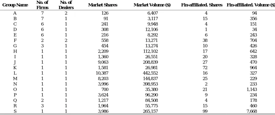
Table 1 is a summary of group-affiliation firms. We select the groups which have at least one dealer firms and one listed firms (excluding the securities firms) as our sample. The first column of the table is the name of the group, the second column is the number of the firms listed on the Taiwan stock exchange within the same affiliated group; and the third column is the number of dealers within the same group. Most of the groups have one listed firms and one dealer firm, while some of groups are relative large. For example, the number of listed firms of A and B is 7, and that of C, D, E is 6.
Column 4 (5) is the averaged daily market trading volume per stock in shares (dollars). As you can see from the two columns, some of the listed firms within the group are actively traded, while some of them are not. For example, the averaged daily trading volume of L Group is NT$ 442 millions (the highest) while that of B is NT$ 3 millions (the lowest). The last two columns are averaged daily dealers’ trades that involve in the intra-group listed firms (per stock) in terms of shares and dollars, respectively. Based on dollar volume, O’s volume is NT$ 1,143,000, (the highest), while D’s volume is NT$ 34,000 (the lowest). The results seem to indicate that the
XIII trading preferences of intra-group affiliated dealers are different from those of the market.
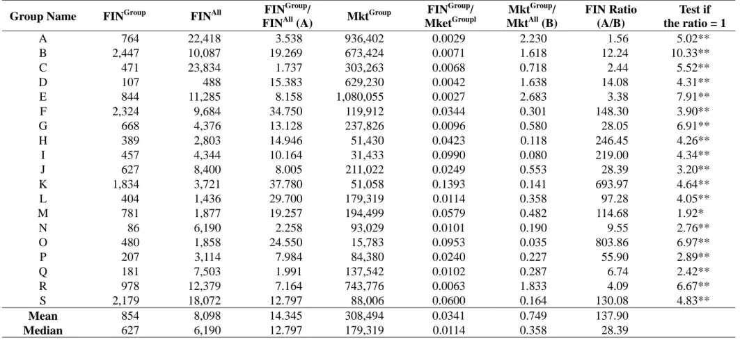
This paper documents trading preference of group-affiliated dealers by standardized the dealers’ trading volume (FIN Ratio) in Table 2. First, since financial institutions may tend to trade more than the other investors, we divide the averaged volume traded on the intra-group stocks(FINGroup)by the affiliated-group’s dealers by the daily averaged volume traded on the non-group-affiliated companies by the dealers (FINAlll), and obtain FINGroup/FINAll in column 4. Likewise, Market
Group
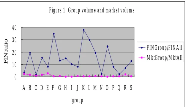
is the daily trading volume for the group in the market averaged across stocks. MarketALL is the total trading volume of the listed firms in the Taiwan stock markets. Thus, we obtain MarketGroup/MarketAll. in column 5. We report the results using trading shares (1,000 shares) in Table 2, and also Figure 1. Figure 1 shows that FINGroup/FINAll and MarketGroup/MarketAll.across all groups. The result indicate that FINGroup/FINAll is higher than MarketGroup/MarketAll.for most of the groups. This indicates that group-affiliated dealers tend to trade heavily on group stocks than that of the other investors.
We also calculate FIN ratio as the relative trading preference of group-affiliated financial institutions, measured by the ratio of FINGroup/FINAll and MarketGroup/MarketAll.. If FIN Ratio is greater than one, we may argue that the intra-group dealers prefer to trade heavily with intra-group stocks. In Table 2, the FIN Ratio varies widely from 1.56 to 803.86. All of FIN Ration is great than one. The mean (median) value of FIN is 137.9 (28.39) in terms of shares. This indicates that financial affiliated dealers trade heavily on the group stocks. We also provide binomial tests to see if the ratio is equal to one in the last column, and the results
XIV indicate that all of the ratios are significantly different from one. Our results suggest that group-affiliated dealers do have trading preferences on intra-group stocks. This paper also calculates the FIN Ratio using dollar volume, and the results are similar and upon request.
Table 3 presents the trading preference by conducting regression models. The affiliated group in our sample exhibit considerable diversity in their group size (proxy by no of stocks listed; Nojstock). Given this diversity, we conduct a regression
analysis to control for the factor mentioned above. Meanwhile, the dependent variable is the FIN Volume contributed by intra-group financial institutions j normalized by the market trading volume for stock k on date t. The independent variables are a dummy for trading preference (Groupj,k =1, if the stock traded is
affiliated with financial institution j ) and the number of listed firms in a group (Nojstock). We run the regression, respectively, for each affiliated group. All of the
coefficients are multiplied by 100.
Table 3 indicates that the coefficients of Group are positive for fourteen out of nineteen groups and the coefficient of number of firms in a group is positive. The coefficient of a pooling regression for all groups is 0.156, and statistically significant different from zero. The finding of Table 3 reveals that after we control for group size, the group-affiliated dealers still have a trading preference on their group stocks. The positive relationship between number of listed firms in a group and the FIN indicates that dealers affiliated with a large group intend to trade group stocks more heavily.
In Table 4, this paper controls for trading volume of Group stocks relative to the whole market in a particular period of time in testing trading preference
XV hypothesis. While, MktGroup i/Index Mktis the trading volume of Group stocks relative to the whole market in a particular period of time. The coefficient of Group is 2.451 and statistically significant, which is larger than that of Table 3, supporting trading preference hypothesis for group-affiliated dealers. However, the coefficients of MktGroup i/Index Mkt are negative, implying that when the trading volume of group stocks are low, group-affiliated dealers tend to involve more in their affiliated groups. One plausible reason is the dealers may be requested to provide liquidity to the group-affiliated stocks when the group-affiliated stocks are less liquid in the market.
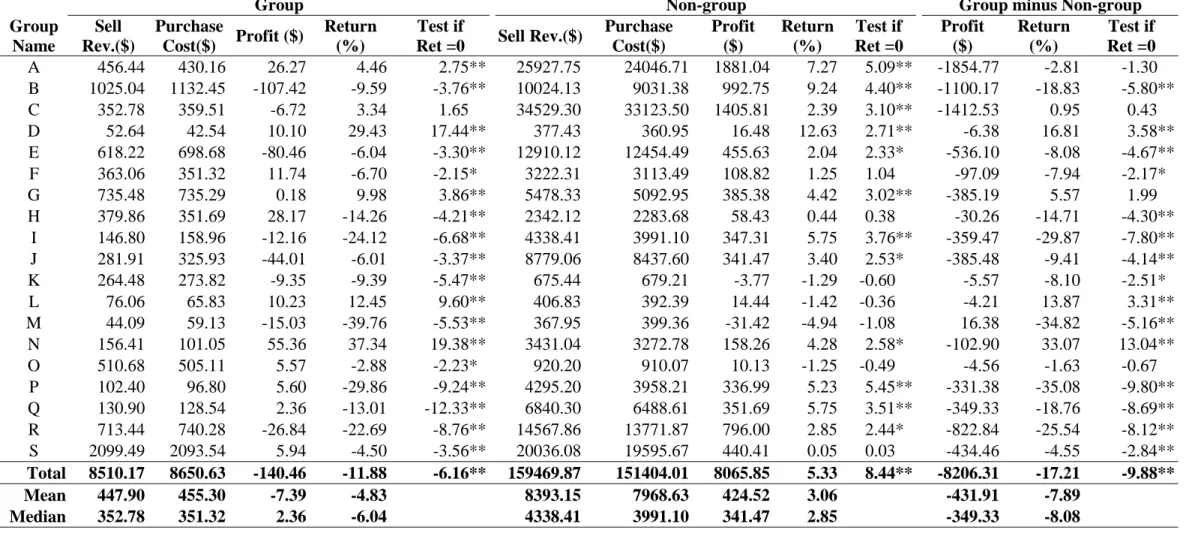
Table 5 reports the trading profits of group-affiliated dealers. The purpose of this table is to compare the performance of affiliated-dealers when they trade with intra-group stocks versus non-group stocks. We calculate the trading performance using dollar profits in millions and returns in percentage at the same time. From Table 5, we find that group-affiliated dealers are unprofitable with trades involving in intra-group stocks; the gross profit in terms of mean dollar profit is -7.39 millions, while in terms of averaged return is –4.83%. As to the trades with non-group stocks, dealers perform relatively well; the gross return is 3.06%, and the dollar profit is 424.52 millions. We also test the differences between dealer profits with trades in group stocks versus non-group stocks, and the gross dollar profit is -431.91 millions and the return is –7.89%. Our findings indicate that dealers did perform well when they trade with non-group stocks. Hence, we document that dealers tend to trade heavily in group-affiliated stocks, yet such kind of trades are unprofitable even before we consider transaction costs. The results support that dealers may have overconfidence toward group-affiliated stocks or they may be required to support liquidity to the listed stocks of their affiliated groups. Therefore, we do not find any
XVI evidence showing that there is any trading profits potential when dealers involve in intra-group stocks. Table 6 provide net profits in millions ($NT) and return in (%). We deduct the gross profits by the transaction tax for selling stocks and commission rate (0.1428) for buys and sells. The results are quite similar to those of Table 5, indicating that dealers tend to lose from trade on group-affiliated stocks.
Table 7 is the gross profits (Panel A) and net profits (Panel B) deducted by market return for group and non-group firms. We also test whether the returns from group and non-group are equal to zero. After adjusting market return, we find that all of the adjusted returns are negative no matter what dealers trade in group-affiliated stocks or non-group-affiliated stocks, and apparently the trading performance of group-affiliated stocks are worse than that of non-group-affiliated stocks. We further run regressions in Table 8 to control for group size, and most of the coefficients of the gross profits, net profits, gross profits adjusted for market returns and net profits adjusted for market returns regressions are negative, basically confirming that affiliated-group dealers encounter loss when they trade in their affiliated stocks.
IV. Conclusions
There is a well-documented home-bias phenomenon in the literature. However, it is unclear whether transaction costs, information asymmetry or overconfidence are the plausible reasons for the home bias. This paper studies that the trading preference of group-affiliated financial firms. Group-affiliated financial firms are supposed to have potential private information and familiarity with their group stocks
XVII than the other financial firms. Our results indicate that group-affiliated dealers do prefer to trade their group stocks after controlling market volume. By conducting trading profits analysis, we consider whether financial institutions are better able to extract private information. The results indicate that affiliated-group dealers encounter loss when they trade in their affiliated stocks. Hence, we may conclude that group-affiliated dealers tend to be overconfidence while they trade group stocks.
XVIII
References
Brennan, Michael J; Cao, H Henry, 1997, “International portfolio investment flows” Journal of Finance 52, 1851-1880.
Christoffersen Susan, and Sergei Sarkiss1an, 2002, “Location overconfidence,”
Mcgill University, Working paper.
Claessens, Stijn; Djankov, Simeon; Lang, Larry H P, 2000, “The separation of ownership and control in East Asian corporations” Journal of Financial
Economics 58, 81-112.
Cooper, Ian; Kaplanis, Evi, 1994, “The implications of the home bias in equity portfolios” Business Strategy Review 5, 41-53.
Coval Joshua D., and Tobias J. Moskowitz, 1999, “Home bias at home: Local equity preference in domestic portfolios” Journal of Finance 54, 2045-2073. Coval Joshua D., and Tobias J. Moskowitz, 2001, “The geography if
investment:Informed trading and asset prices, ” Journal of Political Economy 109, 811-841.
Dahlquist, Magnus; Robertsson, Goran, 2001, “Direct foreign ownership,
institutional investors, and firm characteristics” Journal of Financial Economics
59, 413-440.
Dahlquist Magnus, Lee Pinkowitz, Rene’ M. Stulz, Rohan Williamson, 2002, “Corporate governance and the home bias,” Georgetown University, working
paper.
Daniel, K., D. Hirshleifer, and A. Subramanyam, 1998, “Investor psychology and security market under-and overreactions,” Journal of Finance 53,
1839-1885.
French, Kenneth R; Poterba, James M, 1991, “Investor Diversification and International Equity Markets” American Economic Review, 222-226.
XIX Grinblatt, Mark; Keloharju, Matti, 2001, “How distance, language, and culture
influence stockholdings and trades” Journal of Finance 56, 1053-1073.
Grinblatt, Mark; Keloharju, Matti, 2001, “What makes investors trade?” Journal
of Finance 56, 589
Hau, Harald, 2001, “Location matters: An examination of trading profits”
Journal of Finance 56, 1959-1983.
Huberman, Gur, 1998, “Familiarity breeds investment” Columbia University
working paper.
Glassman, Debra A; Riddick, Leigh A, 1996, “Why empirical international portfolio models fail: Evidence that model misspecification creates home asset bias” Journal of International Money & Finance 15, 275-312.
Glassman, Debra A; Riddick, Leigh A, 1996, “What causes home assets bias and how should it be measured?” Journal of Empirical Finance 8, 35-54.
Kang, Jun-Koo; Stulz, Rene M, 1997, “Why is there a home bias? An analysis of foreign portfolio equity ownership in Japan” Journal of Financial Economics 46, 3-28.
Kang, Jun-Kooa,1; Shivdasani, Anil, 1999, “An analysis of independent and bank-affiliated firms” Pacific-Basin Finance Journal 7, 1-22
Maria Sole Brioschi, Giovanni Marseguerra, Stefano Paleari, 1999, “Corporate Groups and Minority Shareholder Wealth: A Role for Private Benefits?”
Asia-Pacific Financial Markets 6, 355-383.
Odean, T. 1998, “Volume, volatility, price, and profit when all traders are above average,” Journal of Finance 53, 1887-1934.
Pastor, Lubos, 2000, “Portfolio selection and asset pricing models” Journal of
Finance 55, 179-223.
Santis, Giorgio De; Gerard, Bruno, 1997, “International asset pricing and portfolio diversification with time-varying risk” Journal of Finance 52,
XX 1881-1912.
Stockman, Alan C; Dellas, Harris, 1989, “International Portfolio
Nondiversification and Exchange Rate Variability” Journal of International
Economics, 271-289.
Tarun Khanna, Krishna Palepu, 2000, “Is Group Affiliation Profitable in
Emerging Markets? An Analysis of Diversified Indian Business Groups” Journal
of Finance 55, 867-891.
Tesar, Linda La; Werner, Ingrid Mb, 1995, “Home bias and high turnover”
XXI
Figure 1 Group volume and market volume
0
10
20
30
40
A B C D E F G H I J K L M N O P Q R S
group
FI N r a ti oFINGroup/FINAll
MktGroup/MktAll
XXII
TABLE 1 Sample Description
This table shows the number of listed firms (column 2)and that of financial institutions(column 3), respectively, in the same affiliated group. Daily market volume of a specific affiliated group in terms of shares and dollars are shown in columns 4 and 5, respectively. The values in columns 6 (in terms of 1,000 shares)and 7 (in terms of thousands NT$)are the trading volumes made by the financial institutions that were in the same affiliated group. The values in columns 4-7 are divided by no. of dealers and listed firms in the same affiliated group. Daily market volume (Market Vol.) and Dealer volume (Dealer Vol.) are in 1,000 shares ( NT dollars).
Group Name No. of Firms
No. of
Dealers Market Shares Market Volume ($) Fin-affiliated. Shares Fin-affiliated. Volume ($)
A 7 2 126 6,407 4 94 B 7 1 91 3,117 15 356 C 6 1 241 9,948 4 151 D 6 1 308 12,106 1 34 E 6 1 216 8,292 6 243 F 2 2 558 13,271 38 704 G 3 1 454 13,274 10 426 H 1 1 2,209 112,102 17 642 I 1 1 1,360 26,551 20 328 J 1 1 9,063 208,839 27 470 K 1 1 1,581 26,981 72 964 L 1 1 10,387 442,552 16 327 M 1 1 8,203 144,837 25 229 N 1 1 3,996 398,953 2 233 O 1 1 700 35,380 21 1,143 P 1 1 3,624 96,290 9 234 Q 2 1 1,217 84,508 4 178 R 3 1 1,964 55,775 15 460 S 1 1 3,986 265,157 99 7,668
XXIII
TABLE 2 Trading preference of group-affiliated financial institutions
FINGroup is the averaged number of shares traded on the intra-group stocks by the affiliated-group’s financial institutions. FINAlll is the daily averaged number of shares traded on the non-group-affiliated companies by the financial institutions. FINGroup/FINARatio is the ratios of two averages, FINGroup and FINA. Market Group is the daily trading volume for the group in the market averaged across stocks. FINGroup/MarketGroup is the daily trading volume contributed by group-affiliated financial institutions normalized by the market trading volume. MarketALL is the total trading volume of the listed firms in the Taiwan stock markets. FIN ratio is the relative trading preference of group-affiliated financial institutions, measured by the ratio of FINGroup/FINAll and MarketGroup/MarketAll. Market volume (Market Vol.) and Dealer volume (Dealer Vol.) are in 1,000 shares (NTdollars). We use binomial tests to see if the ratio is equal to one. ** represents the significance level of 1%, while * represents the significance level of 5%.
Group Name FINGroup FINAll FIN Group
/
FINAll (A) Mkt
Group FINGroup/ MketGroupl MktGroup/ MktAll (B) FIN Ratio (A/B) Test if the ratio = 1 A 764 22,418 3.538 936,402 0.0029 2.230 1.56 5.02** B 2,447 10,087 19.269 673,424 0.0071 1.618 12.24 10.33** C 471 23,834 1.737 303,263 0.0068 0.718 2.44 5.52** D 107 488 15.383 629,230 0.0042 1.638 14.08 4.31** E 844 11,285 8.158 1,080,055 0.0027 2.683 3.38 7.91** F 2,324 9,684 34.750 119,912 0.0344 0.301 148.30 3.90** G 668 4,376 13.128 237,826 0.0096 0.580 28.05 6.91** H 389 2,803 14.946 51,430 0.0423 0.118 246.45 4.26** I 457 4,344 10.164 31,433 0.0990 0.080 219.00 4.34** J 627 8,400 8.005 211,022 0.0249 0.553 28.39 3.20** K 1,834 3,721 37.780 51,058 0.1393 0.141 693.97 4.64** L 404 1,436 29.700 179,319 0.0114 0.358 97.28 4.05** M 781 1,877 19.257 194,499 0.0579 0.482 114.68 1.92* N 86 6,190 2.258 93,029 0.0101 0.190 9.55 2.76** O 480 1,858 24.550 15,783 0.0953 0.035 803.86 6.97** P 207 3,114 7.984 84,380 0.0240 0.227 55.90 2.89** Q 181 7,503 1.991 137,542 0.0102 0.287 6.74 2.42** R 978 12,379 7.164 743,776 0.0063 1.833 4.09 6.67** S 2,179 18,072 12.797 88,006 0.0600 0.164 130.08 4.83** Mean 854 8,098 14.345 308,494 0.0341 0.749 137.90 Median 627 6,190 12.797 179,319 0.0114 0.358 28.39
XXIV Table 3 Trading preference hypothesis: control for group size
Given this diversity in number of listed firms affiliated with a group, we conduct a regression analysis to control for the factor.
Fin Volj,k,t /Market Vol k,t = a + b1 Groupj,k + b2 Nojstock + ej, k,t
The dependent variables are the FIN Volume contributed by intra-group financial institutions j normalized by the market trading volume for stock k on date t. Groupj,k is a dummy for trading preference; Group=1, if the stock traded is affiliated
with financial institution j. No of stock (Nojstock) means the number of listed firms in
a group. We run the regression, respectively, for each affiliated group. All of the coefficients are multiplied by 100.
Trading Shares (in lots)
Group Name Intercept Group Nojstock AR2
A 0.384** -0.058** x 0.0005 B 0.233** 0.245** x 0.0090 C 0.260** 0.079** x 0.0009 D 0.764** 0.117 x 0.0007 E 0.268** -0.010 x 0.0001 F 0.181** 0.367** x 0.0285 G 0.262** 0.545** x 0.0482 H 0.291** 0.228** x 0.0217 I 0.238** 0.438** x 0.0445 J 0.253** 0.026 x 0.0004 K 0.338** 0.322** x 0.0112 L 0.377** -0.147 x 0.0050 M 0.533** -0.087 x 0.0009 N 0.284** -0.120** x 0.0035 O 0.166* 0.965** x 0.0439 P 0.186** 0.057** x 0.0020 Q 0.242** -0.046* x 0.0009 R 0.222** 0.034* x 0.0005 S 0.298** 0.050** x 0.0010 All Group 0.285** 0.156** -0.049** 0.0278
XXV Table 4 Trading preference: control for the market volume and group size
This table controls for trading volume of Group stocks relative to the whole market in a particular period of time.
Fin Voli/Mkt groupi=a+b1*Group+b2*Mkt groupi /Index Mkt+b3*Nojstock + ei
The dependent variables are the FIN Volume contributed by intra-group financial institutions j normalized by the market trading volume for stock k on date t. Groupj,k is a dummy for trading preference; Group=1, if the stock traded is affiliated
with financial institution j. MktGroup i/Index Mkt is the trading volume of Group stocks relative to the whole market in a particular period of time. No of stock (Nojstock) means the number of listed firms within the same intra-group. We run the
regression, respectively, for each affiliated group. All of the coefficients are multiplied by 100.
Group
Name Intercept Group MktGroup
i /Index Mkt ( Nojstock AR2 A 2.705** -0.103 -102.979** x 0.0405 B 2.245** 0.834** -66.470** x 0.0584 C 1.739** 0.883** -62.302** x 0.0467 D 3.013** 3.384** -98.536** x 0.0856 E 1.379** 0.337** -52.744** x 0.0402 F 1.069** 6.378** -46.758** x 0.1901 G 2.038** 3.544** -70.213** x 0.1051 H 1.726** 2.591** -68.984** x 0.0952 I 2.882** 7.142** -128.722** x 0.1164 J 2.469** 0.556* -75.252** x 0.0526 K 1.453** 12.530** -55.607* x 0.2534 L 1.348** 0.020 -52.281** x 0.0739 M 4.500** 2.050 -159.783** x 0.0601 N 2.614** -1.186* -102.638** x 0.0535 O 1.269** 8.289** -46.776** x 0.3348 P 1.745** 0.938** -61.570** x 0.0699 Q 2.629** -0.475 -102.392** x 0.0466 R 2.268** 1.176** -79.431** x 0.0424 S 3.320** 2.892** -136.802** x 0.0599 All Group 3.083** 2.451** -81.484** -0.261* 0.0684
XXVI
TABLE 5 Gross Profits Calculation
We calculate the selling revenues (Sell Rev) and purchasing costs (Purchase Cost) for each round-trip trade. Trading profits (Profit) is calculated by selling revenues deducted by purchasing costs. Return is measured by the trading profits divided by purchasing costs. Group means the trades that involve in group-affiliated firms made by the financial institutions, while Non-group means the trades that involve in non-group-affiliated firms made by the financial institutions. The paper tests whether return is equal to zero using t tests. ** represents the significance level of 1%, while * represents the significance level of 5%.
Group Non-group Group minus Non-group
Group Name Sell Rev.($) Purchase Cost($) Profit ($) Return (%) Test if
Ret =0 Sell Rev.($)
Purchase Cost($) Profit ($) Return (%) Test if Ret =0 Profit ($) Return (%) Test if Ret =0 A 456.44 430.16 26.27 4.46 2.75** 25927.75 24046.71 1881.04 7.27 5.09** -1854.77 -2.81 -1.30 B 1025.04 1132.45 -107.42 -9.59 -3.76** 10024.13 9031.38 992.75 9.24 4.40** -1100.17 -18.83 -5.80** C 352.78 359.51 -6.72 3.34 1.65 34529.30 33123.50 1405.81 2.39 3.10** -1412.53 0.95 0.43 D 52.64 42.54 10.10 29.43 17.44** 377.43 360.95 16.48 12.63 2.71** -6.38 16.81 3.58** E 618.22 698.68 -80.46 -6.04 -3.30** 12910.12 12454.49 455.63 2.04 2.33* -536.10 -8.08 -4.67** F 363.06 351.32 11.74 -6.70 -2.15* 3222.31 3113.49 108.82 1.25 1.04 -97.09 -7.94 -2.17* G 735.48 735.29 0.18 9.98 3.86** 5478.33 5092.95 385.38 4.42 3.02** -385.19 5.57 1.99 H 379.86 351.69 28.17 -14.26 -4.21** 2342.12 2283.68 58.43 0.44 0.38 -30.26 -14.71 -4.30** I 146.80 158.96 -12.16 -24.12 -6.68** 4338.41 3991.10 347.31 5.75 3.76** -359.47 -29.87 -7.80** J 281.91 325.93 -44.01 -6.01 -3.37** 8779.06 8437.60 341.47 3.40 2.53* -385.48 -9.41 -4.14** K 264.48 273.82 -9.35 -9.39 -5.47** 675.44 679.21 -3.77 -1.29 -0.60 -5.57 -8.10 -2.51* L 76.06 65.83 10.23 12.45 9.60** 406.83 392.39 14.44 -1.42 -0.36 -4.21 13.87 3.31** M 44.09 59.13 -15.03 -39.76 -5.53** 367.95 399.36 -31.42 -4.94 -1.08 16.38 -34.82 -5.16** N 156.41 101.05 55.36 37.34 19.38** 3431.04 3272.78 158.26 4.28 2.58* -102.90 33.07 13.04** O 510.68 505.11 5.57 -2.88 -2.23* 920.20 910.07 10.13 -1.25 -0.49 -4.56 -1.63 -0.67 P 102.40 96.80 5.60 -29.86 -9.24** 4295.20 3958.21 336.99 5.23 5.45** -331.38 -35.08 -9.80** Q 130.90 128.54 2.36 -13.01 -12.33** 6840.30 6488.61 351.69 5.75 3.51** -349.33 -18.76 -8.69** R 713.44 740.28 -26.84 -22.69 -8.76** 14567.86 13771.87 796.00 2.85 2.44* -822.84 -25.54 -8.12** S 2099.49 2093.54 5.94 -4.50 -3.56** 20036.08 19595.67 440.41 0.05 0.03 -434.46 -4.55 -2.84** Total 8510.17 8650.63 -140.46 -11.88 -6.16** 159469.87 151404.01 8065.85 5.33 8.44** -8206.31 -17.21 -9.88** Mean 447.90 455.30 -7.39 -4.83 8393.15 7968.63 424.52 3.06 -431.91 -7.89 Median 352.78 351.32 2.36 -6.04 4338.41 3991.10 341.47 2.85 -349.33 -8.08
XXVII
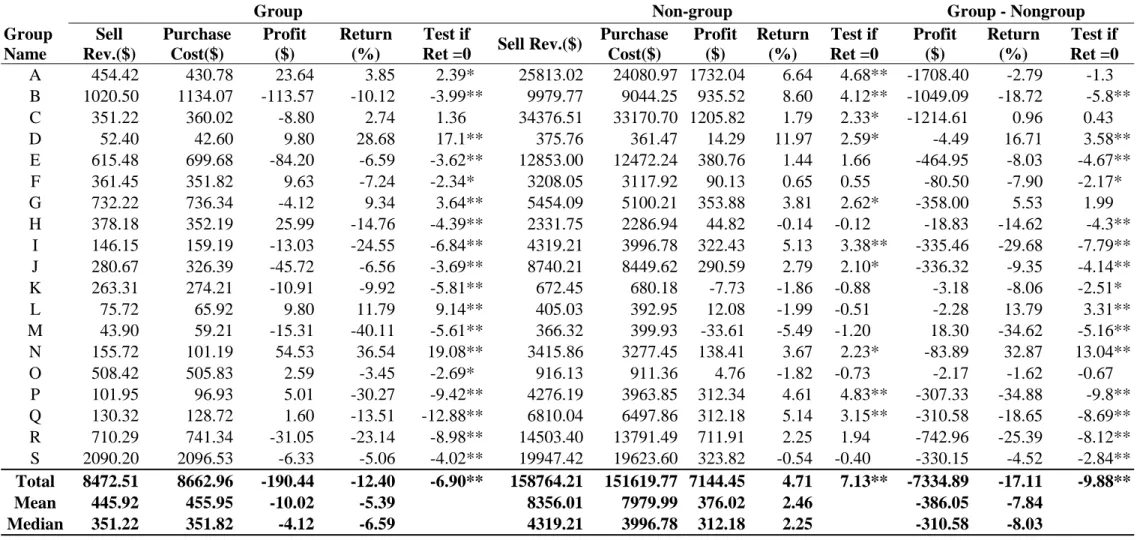
TABLE 6 Net Profits Calculation
We calculate the selling revenues (Sell Rev) and purchasing costs (Purchase Cost) for each round-trip trade. Trading profits (Profit) is calculated by selling revenues deducted by purchasing costs. Return is measured by the trading profits divided by purchasing costs. Group means the trades that involve in group-affiliated firms made by the financial institutions, while Non-group means the trades that involve in non group-affiliated firms made by the financial institutions. Net profits were calculated by the gross profits minus transaction costs in millions. The paper tests whether return is equal to zero using t tests. ** represents the significance level of 1%, while * represents the significance level of 5%.
Group Non-group Group - Nongroup
Group Name Sell Rev.($) Purchase Cost($) Profit ($) Return (%) Test if
Ret =0 Sell Rev.($)
Purchase Cost($) Profit ($) Return (%) Test if Ret =0 Profit ($) Return (%) Test if Ret =0 A 454.42 430.78 23.64 3.85 2.39* 25813.02 24080.97 1732.04 6.64 4.68** -1708.40 -2.79 -1.3 B 1020.50 1134.07 -113.57 -10.12 -3.99** 9979.77 9044.25 935.52 8.60 4.12** -1049.09 -18.72 -5.8** C 351.22 360.02 -8.80 2.74 1.36 34376.51 33170.70 1205.82 1.79 2.33* -1214.61 0.96 0.43 D 52.40 42.60 9.80 28.68 17.1** 375.76 361.47 14.29 11.97 2.59* -4.49 16.71 3.58** E 615.48 699.68 -84.20 -6.59 -3.62** 12853.00 12472.24 380.76 1.44 1.66 -464.95 -8.03 -4.67** F 361.45 351.82 9.63 -7.24 -2.34* 3208.05 3117.92 90.13 0.65 0.55 -80.50 -7.90 -2.17* G 732.22 736.34 -4.12 9.34 3.64** 5454.09 5100.21 353.88 3.81 2.62* -358.00 5.53 1.99 H 378.18 352.19 25.99 -14.76 -4.39** 2331.75 2286.94 44.82 -0.14 -0.12 -18.83 -14.62 -4.3** I 146.15 159.19 -13.03 -24.55 -6.84** 4319.21 3996.78 322.43 5.13 3.38** -335.46 -29.68 -7.79** J 280.67 326.39 -45.72 -6.56 -3.69** 8740.21 8449.62 290.59 2.79 2.10* -336.32 -9.35 -4.14** K 263.31 274.21 -10.91 -9.92 -5.81** 672.45 680.18 -7.73 -1.86 -0.88 -3.18 -8.06 -2.51* L 75.72 65.92 9.80 11.79 9.14** 405.03 392.95 12.08 -1.99 -0.51 -2.28 13.79 3.31** M 43.90 59.21 -15.31 -40.11 -5.61** 366.32 399.93 -33.61 -5.49 -1.20 18.30 -34.62 -5.16** N 155.72 101.19 54.53 36.54 19.08** 3415.86 3277.45 138.41 3.67 2.23* -83.89 32.87 13.04** O 508.42 505.83 2.59 -3.45 -2.69* 916.13 911.36 4.76 -1.82 -0.73 -2.17 -1.62 -0.67 P 101.95 96.93 5.01 -30.27 -9.42** 4276.19 3963.85 312.34 4.61 4.83** -307.33 -34.88 -9.8** Q 130.32 128.72 1.60 -13.51 -12.88** 6810.04 6497.86 312.18 5.14 3.15** -310.58 -18.65 -8.69** R 710.29 741.34 -31.05 -23.14 -8.98** 14503.40 13791.49 711.91 2.25 1.94 -742.96 -25.39 -8.12** S 2090.20 2096.53 -6.33 -5.06 -4.02** 19947.42 19623.60 323.82 -0.54 -0.40 -330.15 -4.52 -2.84** Total 8472.51 8662.96 -190.44 -12.40 -6.90** 158764.21 151619.77 7144.45 4.71 7.13** -7334.89 -17.11 -9.88** Mean 445.92 455.95 -10.02 -5.39 8356.01 7979.99 376.02 2.46 -386.05 -7.84 Median 351.22 351.82 -4.12 -6.59 4319.21 3996.78 312.18 2.25 -310.58 -8.03
XXVIII
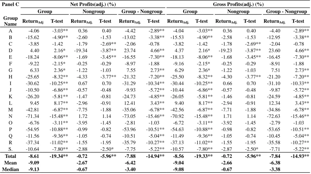
Table 7 Adjusted-Profits Differences
We deduct gross profits (Panel A) and net profits (Panel B) by the market return, and the calculated the differences of the profits between group (with financial-affiliated firms) and nongroup (without financial-affiliated firms). We also test whether the returns from group and nongroup, respectively, are equal to zero. Profits are in millions.
Panel C Net Profits(adj.) (%) Gross Profits(adj.) (%)
Group Nongroup Group - Nongroup Group Nongroup Group - Nongroup Group
Name ReturnAdj T-test ReturnAdj. T-test ReturnAdj. T-test ReturnAdj. T-test ReturnAdj. T-test ReturnAdj. T-test
A -4.06 -3.03** 0.36 0.40 -4.42 -2.89** -4.04 -3.03** 0.36 0.40 -4.40 -2.89** B -15.62 -4.90** -2.60 -1.53 -13.02 -3.38** -15.53 -4.90** -2.58 -1.53 -12.95 -3.38** C -3.85 -1.42 -1.79 -2.69** -2.06 -0.78 -3.82 -1.42 -1.78 -2.69** -2.04 -0.78 D 4.40 2.16* -19.34 -3.87** 23.74 4.66** 4.37 2.16* -19.23 -3.87** 23.60 4.66** E -18.24 -8.06** -1.69 -3.45** -16.55 -7.30** -18.13 -8.06** -1.68 -3.45** -16.45 -7.30** F -9.22 -2.15* -0.25 -0.29 -8.97 -1.88 -9.16 -2.15* -0.25 -0.29 -8.91 -1.88 G 6.33 2.36* -1.22 -1.03 7.55 2.73** 6.29 2.36* -1.22 -1.03 7.51 2.73** H -25.65 -8.32** -4.33 -3.77** -21.32 -7.20** -25.50 -8.32** -4.30 -3.77** -21.20 -7.20** I -30.62 -10.25** 0.67 0.70 -31.29 -10.34** -30.44 -10.25** 0.66 0.70 -31.10 -10.33** J -10.50 -6.86** -0.57 -0.48 -9.93 -5.72** -10.44 -6.86** -0.57 -0.48 -9.87 -5.72** K -26.20 -5.81** -1.47 -0.81 -24.73 -4.85** -26.05 -5.81** -1.46 -0.81 -24.59 -4.85** L 9.45 8.17** -2.96 -0.91 12.41 3.43** 9.40 8.17** -2.94 -0.91 12.34 3.43** M -42.81 -6.87** -7.75 -1.88 -35.06 -6.78** -42.56 -6.87** -7.71 -1.88 -34.86 -6.78** N -71.34 -15.48** 1.72 1.14 -73.05 -15.46** -70.92 -15.48** 1.71 1.14 -72.63 -15.46** O -6.76 -3.11** -3.95 -1.45 -2.81 -1.03 -6.72 -3.11** -3.92 -1.45 -2.79 -1.03 P -54.95 -10.88** -0.99 -0.82 -53.96 -10.51** -54.63 -10.88** -0.98 -0.82 -53.65 -10.51** Q -11.56 -9.36** -1.05 -0.74 -10.51 -5.04** -11.49 -9.36** -1.05 -0.74 -10.45 -5.04** R -37.34 -11.02** -1.55 -1.95 -35.79 -10.27** -37.13 -11.02** -1.55 -1.95 -35.58 -10.27** S. -10.64 -7.80** -2.88 -2.50* -7.75 -5.22** -10.57 -7.80** -2.87 -2.50* -7.71 -5.22** Total -8.61 -19.34** -0.72 -5.96** -7.88 -14.94** -8.56 -19.33** -0.72 -5.96** -7.84 -14.93** Mean -9.09 -2.67 -6.42 -9.04 -2.66 -6.38 Median -9.13 -0.67 -3.40 -9.08 -0.67 -3.38
XXIX Table 8 Profits of group-affiliated financial institutions
We run regressions to control for group size as follows:
Profits=a+b1*Group+b2*No+ e
The dependent variable is the profit in return for financial institution j that involve in stock k (group or non-group) for a sale on date t. Groupj,k is a dummy variable set to 1
if financial institution j involves in the stock k within the same group-affiliated firms on date t. Nojstock means the number of listed firms within the same intra-group.
NojFIN represents the number of financial institutions within the same intra-group. We
run the regression, respectively, for each affiliated group. The coefficients are multiplied by 100. The value in the cell is the coefficients of Group dummy multiplied by 100.
Group Name Gross profits Net profits Gross profits adjusted Net profits adjuested A -2.687 -2.671 -0.377 -0.375 B -12.200** -12.129** -1.654* -1.645* C -4.457** -4.428** -10.689** -10.626** D 10.552 10.49 29.419** 29.247** E -12.734** -12.660** -18.927** -18.817** F 0.164 0.163 3.627** 3.606** G -4.728* -4.701* 2.082** 2.070** H 4.685** 4.658** -0.937* -0.931* I -8.165** -8.111** -9.384** -9.328** J -17.31** -17.209** -21.341** -21.217** K -4.225** -4.200** -2.888** -2.871** L 11.016* 10.951* 9.568** 9.512** M -5.961 -5.926 -11.304** -11.237** N 48.188** 47.906** -16.654** -16.556** O -1.544 -1.535 3.704** 3.682** P -5.672 -5.639 5.937** 5.902** Q -4.551 -4.524 2.934 2.917 R -14.478** -14.391** -12.234** -12.162** S -5.388** -5.356** 1.983** 1.971** All Group -5.609** -5.576** -3.866** -3.843**