改善FP-growth資料挖掘演算法在巨大資料庫的效能

全文

(1)國立高雄大學資訊工程學系(研究所) 碩士論文. 改善 FP-growth 資料挖掘演算法在巨大資料庫的效能 Improving the Performance of the FP-Growth Mining Algorithm in Very Large Databases. 研究生：黃正男撰指導教授：洪宗貝. 中華民國九十八年七月 I.

(2) Acknowledgements 在研究所的學習過程中，首先感謝我的指導教授洪宗貝教授，在洪老師細心的指導下，讓我學會如何去思考解決問題及撰寫論文的方法，且不辭辛勞的修改論文。在老師指導下，使我在短短二年間能有成長與收穫，同時順利取得碩士學位，在此致上由衷的敬意與感謝！接著我要感謝我的碩士論文口試委員：本校資工系林文揚教授、成功大學資工所曾新穆、高雄第一科技大學曾守正教授於口試期間給予的建議與指教，並於口試期間給予我寶貴的指導與意見，使我的論文更趨完整。接著要感謝好友卓翰、志偉、博正、欣怡、升馨，在口試前互相的鼓勵與協助，使我口試順利完成。同時感謝研究室學長及學弟: Jerry、俊豪、國誠、韋体、廷一、偉屏。雖然每星期只有短短的幾小時 meeting，卻是我最開心快樂的時光，讓研究生涯更為深刻及難忘。最重要的是感謝我的父母，謝謝您們給我無後顧之憂的求學生涯，讓我可以全心投入研究，每當遇到困難或是開心事情時，總是願意傾聽給予意見，在此表達衷心的謝意。最後，這兩年來真的很感謝大家的支持與協助，才能順利完成研究所學業，在此致上我最深的謝意。黃正男. 謹致民國 98 年 7 月. I.

(3) Improving the Performance of the FP-Growth Mining Algorithm in Very Large Databases. Advisor: Dr. Tzung-Pei Hong Department of Computer Science and Information Engineering National University of Kaohsiung Student: Jheng-Nan Huang Department of Computer Science and Information Engineering National University of Kaohsiung ABSTRACT Along with the progress of information techniques and the increase of information need, some databases in the real world grow very quickly and their sizes become very huge. If the FP-Growth procedure is directly executed on these databases to mine association rules, the computer memory may not allow all nodes of a FP-tree generated from a huge database. This means the FP-Growth procedure will be inefficient because of the high page fault rate in the mining process. The thesis thus focuses on solving or easing off the mining problems incurred from memory limitation. A sophisticated mining approach with a flexible partition of items is proposed to effectively derive association rules under the constraint of memory limitation. The proposed approach can be divided into three phases. In the first phase, the domain items that appear in a transaction database are divided into a set of groups under the constraint that the number of items in each group cannot exceed a threshold. The groups in the partition may thus be independent or dependent according to the given data. In the second phase, we slightly modify the FP-tree structure by keeping II.

(4) the transaction numbers for each branch to effectively handle the cross-group mining problem. A modified FP tree is first built from each group of items and the FP-Growth procedure mine the frequent itemsets in individual groups. A compact representation for the frequent itemsets from each group is then designed to save the storage of itemsets. In the third phase, the frequent itemsets in the groups are then merged with the aid of the encoded representation. The proposed approach can make the partition flexible and balanced, thus causing the mining process under the memory limitation always feasible.. Keywords: data mining, association rule, FP-growth, very large database.. III.

(5) 改善 FP-growth 資料挖掘演算法在巨大資料庫的效能指導教授：洪宗貝博士國立高雄大學資訊工程所學生：黃正男國立高雄大學資訊工程所. 摘要. FP-growth 對於從交易資料庫裡挖掘關聯規則而言是一個非常重要的方法，但其在挖掘頻繁項目集前，需要先將在交易資料庫裡的所有挖掘頻繁項目建立成一樹狀結構(FP-tree)，並且保留這個樹狀結構在記憶體。在挖掘關聯規則的過程中如果電腦的記憶體不足，則會許多的硬碟存取動作導致 FP-growth 演算法的效率不佳。在這篇論文我們針對 FP-Growth 的記憶體問題提出一個演算法，以改善 FP-growth 演算法在巨大資料庫的效能。我們所提的演算法分成 3 部分，在第一部分我們會先將交易資料庫的物品項目，分成許多群，而每一群的項目數目都小於一個由使用者根據記憶體大小自行決定的門檻值。在第二部分我們針對每群的項目進行 FP-Growth，以便挖掘出各部分的頻繁項目集，而在挖掘的過程中我們修改原來的樹狀架構以有效找尋頻繁項目集所出現的交易編號，並使用一個壓縮表示法來表示這些尋頻繁項目集和交易編號。在第三部分，我們則利用這些壓縮的頻繁項目集和交易編號，去整合出所有跨群的頻繁項目集。我們所提的方法可以使得項目分群更平衡及更彈性，並且可以解決在尋找頻繁項目集過程中的記憶體問題。關鍵字：資料挖掘、關聯規則、FP-growth、巨大資料庫。. IV.

(6) CONTENTS ENGLISH ABSTRACT ................................................................................................ II CHINESE ABSTRACT ...............................................................................................IV CONTENTS.................................................................................................................. V List of Figures ..............................................................................................................VI List of Tables ............................................................................................................. VIII CHAPTER 1 Introduction.............................................................................................. 1 1.1 Background and Motivation ............................................................................ 1 1.2 Contributions.................................................................................................... 4 1.3 Thesis Organization ......................................................................................... 5 CHAPTER 2 Literature Survey ..................................................................................... 7 2.1 The FP-Growth Algorithm ............................................................................... 7 2.1.1 Construction of an FP-tree .................................................................... 7 2.2 The Domain Item Grouping Algorithm ......................................................... 15 2.3 The Database Projection Algorithm ............................................................... 17 CHAPTER 3 Item Partition by Tree Search ................................................................ 20 3.1 The Proposed Algorithm ................................................................................ 20 3.2 An Example .................................................................................................... 25 CHAPTER 4 Item Partition by Genetic Algorithms .................................................... 31 4.1 The Proposed Algorithm ................................................................................ 31 CHAPTER 5 Generation of Frequent Itemsets from a Partition of Items ................... 41 5.1 The Modified FP Tree.................................................................................... 41 5.2 The Enumeration Tree ................................................................................... 47 5.3 Compacted Frequent Itemsets ........................................................................ 49 5.4 Reconstructing the Enumeration Tree from CFIs .......................................... 54 5.5 Generating the Frequent Itemset Table from a Partitions of Items ................ 55 CHAPTER 6 Finding Cross-Group Frequent Itemsets ................................................ 57 6.1 The Proposed Algorithm .......................................................................... 57 CHAPTER 7 Conclusions............................................................................................ 71 References .................................................................................................................... 73. V.

(7) List of Figures Figure 2-1: The FP-tree after the first transaction is processed ............................ 10 Figure 2-2: The FP-tree after the second transaction is processed........................ 11 Figure 2-3: The resulting Header_Table and FP-tree in the example ................... 11 Figure 2-4: The conditional FP-tree for item p ....................................................... 13 Figure 2-5: The conditional FP-tree for item m ...................................................... 14 Figure 2-6: The conditional FP-tree for item am .................................................... 15 Figure 3-1: The search tree to divide a big group into small sub-groups ............. 28 Figure 4-1: The initial constant order of the items in the example ....................... 34 Figure 4-2: The transformation from a chromosome to a partition ..................... 36 Figure 4-3: The execution process of the transformation procedure .................... 38 Figure 5-1: The MFPT after the first transaction is processed ............................. 44 Figure 5-2: The MFPT after the second transaction is processed ......................... 45 Figure 5-3: The MFPT after the third transaction is processed ............................ 45 Figure 5-4: The final MFPT ...................................................................................... 46 Figure 5-5: The final FPT for a comparison ............................................................ 46 Figure 5-6:The enumeration tree for representing the execution order of the modified FP-Growth procedure ............................................................ 47 Figure 5-7: The pruned enumeration tree ............................................................... 48 Figure 5 8: All the CFIs from the enumeration tree in Figure 5-6 ........................ 51 Figure 5-9: An example for finding transaction IDs from a MFPT ...................... 54 Figure 5-10: The reconstruction process of a path from a CFI ............................. 55 Figure 6-1: Merge of FIT(A, B, C), FIT(D, E, F), FIT(G, H, I) and FIT(J, K)..... 57 Figure 6-2: Using a prefix tree to enumerate all the combinations of the frequent itemset tables .............................................................................................................. 58 Figure 6-3: An incremental merging approach for FIT operations ...................... 59 Figure 6-4: Pruning the superset of FIT(A, B, C) X FIT(D, E, F) ......................... 61 Figure 6-5: Merge CFI1 and CFI2............................................................................. 63 Figure 6-6: An example for finding all the missing frequent itemsets .................. 64 Figure 6-7: Check whether the itemsets (AD, ADE, ADEF) are frequent or not . 64 Figure 6-8: Check whetherthe itemsets (ABD, ABDE, ABDEF) are frequent or not ................................................................................................................................ 65 Figure 6-9: Check whether the itemsets (ABCD, ABCDE, ABCDEF) are frequent VI.

(8) or not ........................................................................................................................... 65 Figure 6-10 : Merge CFI({ABC}(…)) and CFI({ABC}(…)) .................................. 66 Figure 6-11: The content of FITall after merging FIT(D, E, F) and FIT(A, B, C) 66. VII.

(9) List of Tables Table 2-1: A database with five transactions ............................................................. 8 Table 2-2: All the items with their counts .................................................................. 9 Table 2-3: The transactions with only sorted large items......................................... 9 Table 2-4: The transaction database in the example............................................... 16 Table 2-5: All the 2-itemsets in the transaction database ....................................... 16 Table 2-6: The merging process in the example ...................................................... 17 Table 3-1: The transaction database in the example............................................... 25 Table 3-2: All the 2-itemsets in the transaction database ....................................... 26 Table 3-3: The merging process in the example ...................................................... 26 Table 3-4: All the 2-itemsets and their scores from the items in the big group .... 29 Table 4-1: An example for a chromosome................................................................ 37 Table 4-2: All infrequent 2-itemsets of group ({A, B, C, D, E, F, G, H}) ............... 39 Table 4-3: An example for crossover ........................................................................ 40 Table 4-4: An example for mutation......................................................................... 40 Table 5-1: The transaction data set used as the example ....................................... 43. VIII.

(10) CHAPTER 1 Introduction 1.1 Background and Motivation Years of effort in data mining have produced a variety of efficient techniques. Depending on the type of databases processed, these mining approaches may be classified as working on transaction databases, temporal databases, relational databases, and multimedia databases, among others. On the other hand, depending on the class of knowledge derived, the mining approaches may be classified as finding association rules, classification rules, clustering rules, and sequential patterns [4], among others. Among them, finding association rules in transaction databases is most commonly seen in data mining [1][5][6][7][8][9][10][11][12]. In the past, many algorithms for mining association rules from transactions were proposed, most of which were based on the Apriori algorithm [1], which generated and tested candidate itemsets level by level. This may cause iterative database scan and high computational cost. Han et al. thus proposed the Frequent-Pattern-tree (FP-tree) structure for efficiently mining association rules without generation of candidate itemsets [2]. The FP-tree [2] was used to compress a database into a tree structure which stored only large items. It was condensed and complete for finding all 1.

(11) the frequent patterns. The construction process was executed tuple by tuple, from the first transaction to the last one. After that, a recursive mining procedure called FP-Growth was executed to derive frequent patterns from the FP-tree. They showed the approach could have a better performance than Apriori. Along with the progress of information techniques and the increase of information need, some databases in the real world grow very quickly and their sizes become very huge. If the FP-Growth procedure is directly executed on these databases to mine association rules, the computer memory may not allow all nodes of a FP-tree generated from a huge database. This means the FP-Growth procedure will be inefficient because of the high page fault rate in the mining process. Han et al. then proposed the concept of database projection [4] to solve the memory problem. Their approach used “data copy” to generate a set of independent databases, with the number of domain items in each database smaller than a threshold β , which is indicated by users. The approach needs many IO operations and extra disk space in building independent databases. Nan et al. then proposed the concept of grouping domain items [3] to solve the memory problem. Their approach first calculated all frequent 2-itemsets, which were then used to divide the items into a set of independent groups, which meant that there were no frequent itemsets across the groups. The sizes of the groups might, however, 2.

(12) be very unbalanced, thus it is possible for a group to be still too large to be handled due to the memory limitation. The thesis thus focuses on solving or easing off the mining problems incurred from memory limitation. A sophisticated mining approach with a flexible partition of items is proposed to effectively derive association rules under the constraint of memory limitation. The proposed approach can be divided into three phases. In the first phase, the domain items that appear in a transaction database are divided into a set of groups under the constraint that the number of items in each group cannot exceed a threshold. The purpose of the phase is to assure the processing can satisfy the memory limitation. The groups in the partition may thus be independent or dependent according to the given data. Two methods are proposed to partition the items. The first one is based on the branch-and-bound search strategy to find the best partition under the criterion that the cross-group itemsets should be the least. Due to its high time complexity, a heuristic partition method based on genetic algorithms is then proposed. The proposed approach designs a new indirect coding scheme to effectively avoid redundant search. In the second phase, we slightly modify the FP-tree structure by keeping the transaction numbers for each branch to effectively handle the cross-group mining problem. A modified FP tree is first built from each group of items and the FP-Growth procedure mine the frequent itemsets in individual 3.

(13) groups. A compact representation for the frequent itemsets from each group is then designed to save the storage of itemsets. In the third phase, the frequent itemsets in the groups are then merged with the aid of the encoded representation. The proposed approach can make the partition flexible and balanced, thus causing the mining process under the memory limitation always feasible.. 1.2 Contributions The contributions of this thesis are stated in this section. They include the following. 1.. An effective algorithm based on the branch-and-bound strategy is proposed to find an appropriate item partition from a transaction database. The proposed algorithm will first find an independent partition and then divide the partition into a finer one if the item number in a group is too large. An evaluation criterion is designed to achieve the purpose. The proposed approach can thus flexibly guarantee that the mining process within each group of items can be easily handled within the memory limitation.. 2.. An efficient GA-based partition algorithm is proposed to speed up the execution time of the first approach. It can divide each big group into a set of small groups quickly by sacrificing a little accuracy. A trade-off between accuracy and 4.

(14) computation cost can easily be achieved in this way. 3.. The modified FP-tree (MFPT) is proposed to make the mining process from partitioned items easy to perform. It can help search the transactions in which a query itemset appears.. 4.. A new representation is designed to code all the frequent itemsets and their appearing transactions in an impact way. It needs a smaller memory space than before to represent all the contents generated by the FP-Growth procedure.. 5.. A cross-group mining process is designed to integrate the mining results from individual groups of items. All missed frequent itemsets across dependent groups can be efficiently found out.. 1.3 Thesis Organization The remaining parts of this thesis are organized as follows. Some related researches including FP-growth, item partition and database projection are reviewed in Chapter 2. The proposed two methods for dividing a big group into a set of smaller dependent groups are shown in Chapters 3 and 4. The new representation designed to effectively encode frequent itemsets and its construction approach are explained in Chapters 5. The merging approach for finding all frequent itemsets across dependent groups is described in Chapters 6. Conclusion and future works are finally given in 5.

(15) Chapter 7.. 6.

(16) CHAPTER 2 Literature Survey In this chapter, some important concepts related to this thesis are briefly reviewed. They include FP-Growth, domain item grouping, and database projection.. 2.1 The FP-Growth Algorithm Han et al. proposed the Frequent-Pattern-tree structure (FP-tree) for efficiently mining association rules without generation of candidate itemsets [2]. The FP-tree mining algorithm consists of two phases. The first phase focuses on constructing the FP-tree from the database, and the second phase focuses on deriving frequent patterns from the FP-tree. They are described below.. 2.1.1 Construction of an FP-tree. The FP-tree [2] is used to compress a database into a tree structure storing only large items. It is condensed and complete for finding all the frequent patterns. Three steps are involved in FP-tree construction. The database is first scanned to find all items with their frequency. The items with their supports larger than a predefined minimum support are selected as large 1-itemsets (items). Next, the large items are 7.

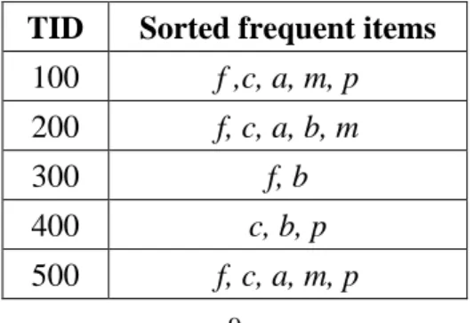
(17) sorted in descending frequency. At last, the database is scanned again to construct the FP-tree according to the sorted order of large items. The construction process is executed tuple by tuple, from the first transaction to the last one. After all transactions are processed, the FP-tree is completely constructed. The Header_Table is also built to help tree traversal. The Header_Table includes the sorted large items and their pointers (called frequency head) linking to their first occurrence nodes in the FP-tree. If more than one node has the same item name, they are also linked in sequence. Note that the links between nodes are single-directional from parents to children. Below, a simple example is given to illustrate the process of the FP-tree construction. Assume there are five transactions shown in Table 2-1. Also assume the minimum support is set at 50%. The FP-tree is constructed in the following way.. Table 2-1: A database with five transactions TID. Items. 100. a, c, d, f, g, i, m ,p. 200. a, b, c, f, l ,m, o. 300. b, f, h, j, o. 400. b ,c, k, s, p. 500. a, c, e, f, l, m, n, p. First, the database is scanned to find large items. All the items with their counts. 8.

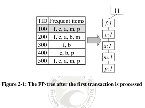
(18) are shown in Table 2-2, in which the large items are marked.. Table 2-2: All the items with their counts Item. frequency. item. frequency. a. 3. j. 1. b. 3. k. 1. c. 4. l. 2. d. 1. m. 3. e. 1. n. 1. f. 4. o. 2. g. 1. p. 3. h. 1. s. 1. i. 1. w. 1. From Table 2-2, it can be observed that the set of large 1-itemsets, named L1, includes {a:3, b:3, c:4, f:4, m:3, p:3}, where the number after an item represents its count. Next, the items in L1 are sorted according to their descending frequency. The sorted L1, named L1’, is {f:4, c:4, a:3. b:3, m:3, p:3}. At last, the database is scanned again to construct the FP-tree. The transactions with only sorted large items are shown in Table 2-3 for illustrating the construction process easily.. Table 2-3: The transactions with only sorted large items TID. Sorted frequent items. 100. f ,c, a, m, p. 200. f, c, a, b, m. 300. f, b. 400. c, b, p. 500. f, c, a, m, p 9.

(19) In Table 2-3, the first transaction is (f, c, a, m, p). The root of the FP-tree is first set Null. This transaction is then inserted into the FP-tree as the first branch. Each node in the branch is attached a count of 1. The results after the first transaction is processed are shown in Figure 2-1.. {} TID Frequent items 100 f, c, a, m, p 200 f, c, a, b, m 300 f, b 400 c, b, p 500 f, c, a, m, p. f:1 c:1 a:1 m:1 p:1. Figure 2-1: The FP-tree after the first transaction is processed. The second transaction is next processed. It shares the same prefix (f, c, a) as the first branch of the FP-tree. The counts of nodes f, c and a are then incremented by 1, and a new node (b:1) is created and linked to (a:2) as its child. Another new node (m:1) is then created and linked to (b:1). Besides, a link is created between the two nodes of m. The results after the second transaction is processed are shown in Figure 2-2.. 10.

(20) {} TID Frequent items 100 f, c, a, m, p 200 f, c, a, b, m 300 f, b 400 c, b, p 500 f, c, a, m, p. f:2 c:2 a:2 m:1 b:1 p:1 m:1. Figure 2-2: The FP-tree after the second transaction is processed. The same process is then executed for the other transactions. After all the transactions are processed, the resulting Header_Table and FP-tree are shown in Figure 2-3.. {} f:4. Header Table Item. c:1. frequency head. c:3. f c a b m p. b:1. a:3. b:1 p:1. m:2. b:1. p:2. m:1. Figure 2-3: The resulting Header_Table and FP-tree in the example. 11.

(21) 2. 1. 2 Mining of Large Itemsets After the FP-tree is constructed from a database, a mining procedure called FP-Growth [12] is executed to find all large itemsets. FP-Growth does not need to generate candidate itemsets for mining, but derives frequent patterns directly from the FP-tree. It is a recursive process, handling the frequent items one by one and bottom-up according to the Header_Table. A conditional FP-tree is generated for each frequent item, and from the tree the large itemsets with the processed item can be recursively derived. Specifically, a conditional FP-tree is generated in the following way. Let a prefix path of an item I in the FP-tree be the preceding part of a branch above I. The corresponding prefix paths for a large item I are first extracted from the FP-tree. The count of each node in a prefix path is set as the count of I in the same branch. The counts of an item appearing in different prefix paths are then summed up. The items with their counts larger than or equal to the minimum count are then selected to build the conditional FP-tree for I. Each prefix path, like a transaction, is used to build the conditional FP-tree as in the FP-tree construction. A conditional FP-tree is thus a little like a sub-FP-tree with the processed item lying at its leaves. An itemset composed of the original item I and each item in the conditional FP-tree is thus certainty large. The process is recursively executed until all the items in a conditional FP-tree are processed. 12.

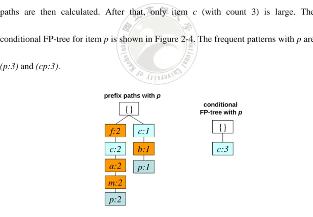
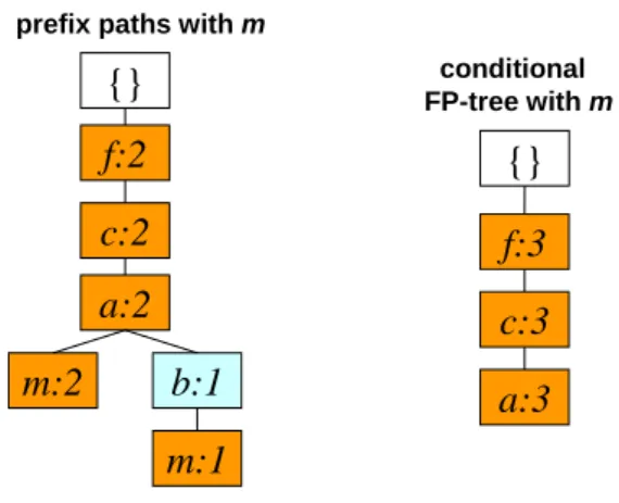
(22) Below, the FP-tree formed in the previous example is used to illustrate the FP-Growth procedure. The frequent items in the Header_Table in Figure 2-3 are processed bottom-up and one by one. Item p is first processed. Two prefix paths exist for item p: (f:4)(c:4)(a:3)(m:2)(p:2) and (c:1)(b:1)(p:1). The counts of all the nodes in the first prefix path are then updated as 2 since they appear only twice with item p in the branch. Similarly, the counts of the nodes in the second prefix path are all updated as 1 since they appear only once with item p. Thus, two converted prefix paths are (f:2)(c:2)(a:2)(m:2) and (c:1)(b:1). The counts of the items in the two prefix paths are then calculated. After that, only item c (with count 3) is large. The conditional FP-tree for item p is shown in Figure 2-4. The frequent patterns with p are (p:3) and (cp:3). prefix paths with p conditional FP-tree with p. {} f:2. c:1. {}. c:2. b:1. c:3. a:2. p:1. m:2 p:2 Figure 2-4: The conditional FP-tree for item p. 13.

(23) Next, item m is processed. There are two converted prefix paths for item m: (f:2)(c:2)(a:2) and (f:1)(c:1)(a:1)(b:1). Only the counts of items f, c and a are larger than or equal to the minimum count (3). The set of large items for the conditional FP-tree of item m are thus {f, c, a}. The conditional FP-tree for item m is then generated by inserting the prefix paths with only the large items one by one. The results are shown in Figure 2-5. prefix paths with m. m:2. {}. conditional FP-tree with m. f:2. {}. c:2. f:3. a:2. c:3 b:1. a:3. m:1 Figure 2-5: The conditional FP-tree for item m. The frequent patterns with m are (m:3), (am:3), (cm:3) and (fm:3). A conditional FP-tree is then recursively constructed in the sequence of am, cm, and fm. The prefix path for am is (f:3)(c:3). The conditional FP-tree for am is shown in Figure 2-6. The large itemsets with am are (am:3), (cam:3) and (fam:3).. 14.

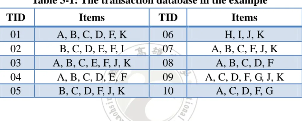
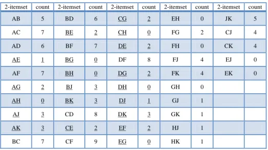
(24) conditional FP-tree with m. {}. conditional FP-tree with am. {} f:3 f:3 c:3 c:3. a:3. Figure 2-6: The conditional FP-tree for item am. The same process is then recursively executed to find all the conditional FP-trees, and to derive the large itemsets from the trees. After all the items on the conditional FP-tree of m have been processed, the following frequent patterns with m are derived: (m:3), (fm:3), (cm:3), (am:3), (fcm:3), (fam:3), (cam:3) and (fcam:3). All the other frequent items in the Header_Table can be processed in the same way.. 2.2 The Domain Item Grouping Algorithm Nan et al. proposed the domain item grouping algorithm to solve the memory problem. The method calculates all frequent 2-itemsets and uses the 2-itemsets to divide the domain items as a set of independent groups. The independent groups mean that there are not any frequent itemsets between the groups. In this section, an example is given to demonstrate their algorithm. This is a simple example to show how the proposed algorithm can be easily used to find an appropriate item partition from a transaction database. The proposed algorithm will find an independent partition. Assume the ten transactions shown in Table 2-4 are used as the example. 15.

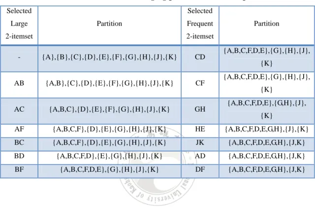
(25) Table 2-4: The transaction database in the example TID. Items. TID. Items. 01 02 03 04 05. A, B, C, D, F, K B, C, D, E, F, I A, B, C, E, F, J, K A, B, C, D, E, F B, C, D, F, J, K. 06 07 08 09 10. H, I, J, K A, B, C, F, J, K A, B, C, D, F A, C, D, F, G, J, K A, C, D, F, G. Assume there are 10 items, A to J, to be purchased in the domain. Also assume the predefined min_support is 5. All the 2-itemsets are then generated from the items and the ones with their counts equal to or larger than 4 are frequent 2-itemsets. Table 2-5 shows all the 2-itemsets generated from the transaction databases. The 2-itemsets without the underline in the table are frequent.. Table 2-5: All the 2-itemsets in the transaction database 2-itemset. count. 2-itemset. count. 2-itemset. count. 2-itemset. count. 2-itemset. count. AB. 5. BD. 6. CG. 2. EH. 0. JK. 5. AC. 7. BE. 2. CH. 0. FG. 2. CJ. 4. AD. 6. BF. 7. DE. 2. FH. 0. CK. 4. AE. 1. BG. 0. DF. 8. FJ. 4. EJ. 0. AF. 7. BH. 0. DG. 2. FK. 4. EK. 0. AG. 2. BJ. 3. DH. 0. GH. 0. AH. 0. BK. 3. DJ. 1. GJ. 1. AJ. 3. CD. 8. DK. 3. GK. 1. AK. 3. CE. 2. EF. 2. HJ. 1. BC. 7. CF. 9. EG. 0. HK. 1. Then the frequent 2-itemsets are used to find the independent partition of the items. If two items belong to the same frequent 2-itemset, they will be put into the same group. Initially, each item forms its own group. Then each frequent 2-itemset is used to merge two groups if the two items in the itemset belong to different groups. For instance, a frequent 2-itemset {A, B} is formed in the example. It will be used to 16.

(26) merge the two groups {A} and {B} together. Table 2-6 shows the merging process in the example. The two groups, {A, B, C, D, E, F, G, H} and {J, K}, in the final partition are thus independent.. Table 2-6: The merging process in the example Selected Large. Selected Partition. Frequent. 2-itemset. Partition. 2-itemset {A,B,C,F,D,E},{G},{H},{J},. -. {A},{B},{C},{D},{E},{F},{G},{H},{J},{K}. CD. AB. {A,B},{C},{D},{E},{F},{G},{H},{J},{K}. CF. AC. {A,B,C},{D},{E},{F},{G},{H},{J},{K}. GH. AF. {A,B,C,F},{D},{E},{G},{H},{J},{K}. HE. {A,B,C,F,D,E,G,H},{J},{K}. BC. {A,B,C,F},{D},{E},{G},{H},{J},{K}. JK. {A,B,C,F,D,E,G,H},{J,K}. BD. {A,B,C,F,D},{E},{G},{H},{J},{K}. AD. {A,B,C,F,D,E,G,H},{J,K}. BF. {A,B,C,F,D,E},{G},{H},{J},{K}. DF. {A,B,C,F,D,E,G,H},{J,K}. {K} {A,B,C,F,D,E},{G},{H},{J}, {K} {A,B,C,F,D,E},{G,H},{J}, {K}. 2.3 The Database Projection Algorithm Han et al. proposed the database projection concept to solve the problem that the memory size of a FP-tree is bigger than the memory. The method uses “data copy” to generate a set of independent databases and the number of domain items in every independent database must be smaller than a threshold β, which is indicated by users. In this section, an example is given to demonstrate the proposed algorithm. Assume the ten transactions database is shown in Table2-4, the value of the threshold β is 5 and the min_support is 4.. 17.

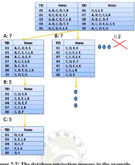
(27) Figure 2-7 shows the database projection of Table 2-4. In the example, we must first search for the transactions that have item A and then delete item A from the transactions. The contents of the transactions are then shown at the left branch of Table (A: 7) of the tree in Figure 2-7. Because the number of domain items in Table (A: 7) is 8, bigger than 5, we must generate the subtable (B: 5) in Figure 2-7. The subtable consists of the transactions that include item B in Table (A: 7), and deletes the item B from the transactions. Because the number of domain items in Table (B: 5) is 6, still bigger than 5, we must use the similar method to generate the subtable (C: 5). because the number of domain items in Table (C: 5) is 5, we do not generate any subtables at the branch. In the example, If we use FP-Growth to mine frequent itemsets from Table (C: 5), the itemsets generated must be a superset of the itemset ABC. Note that in the process that generates subtables, if the count of the appearing items is smaller than min_support, then the subtable for the item cannot be generated. For example, the count of item I is 2, less than min_support, Tables (I :2) does not be generated.. 18.

(28) Figure 2-7: The database projection process in the example. 19.

(29) CHAPTER 3 Item Partition by Tree Search 3.1 The Proposed Algorithm INPUT: 1.. A set of n transactions in a database with a set of m items {I1, I2, …, Im} named DIL (Domain Item List);. 2.. A minimum support threshold named min_support.. 3.. A number threshold β for constraining the number of items in each group of a partition.. OUTPUT: 1.. A proper partition P from the DIL with the item number in each group equal to or less than β.. 2.. The association relations between each big group and its refined sub-groups.. The proposed item-partition algorithm: PHASE 1: STEP 1: Generate all the 2-itemsets from the given items and calculate their counts. STEP 2: If the count of an itemset is larger than the threshold, min_support, then put it in the set of frequent 2-itemsets (FI). STEP 3: Initially set the partition P to have m groups, with each consisting of only one item in DIL. STEP 4: The two groups with the two items in a frequent 2-itemset will be merged 20.

(30) together if they belong to different groups for dependency consideration. STEP 5: Repeat the above step (STEP 4) until there is no frequent 2-itemsets or only one group in the partition. STEP 6: Output the partition into Phase 2 for possible finer division. PHASE 2: STEP 7: If in the partition there is at least one big group (with the item number larger than the number threshold β), do the next step; otherwise, exit the algorithm and output the partition. STEP 8: Use the “Refine-partition” procedure, which is based on the branch-and -bound strategy, to divide each big group into a set of small groups (with their item numbers equal to or smaller than β). STEP 9: Set the association relations between each big group and its refined sub-groups for the usage of later mining. STEP 10: Output the final partition and the association relations between each big group and its refined sub-groups.. Note that after step 10, a proper partition with no or little inter-group dependency can be found. The partition may then be used to improve the efficiency of data mining under some situations. For example, mining association rules under memory limitation in a good application of it. Next, the “Refine-Partition” procedure, which divides each big group into a set of small groups, is introduced. Basically, it is based on the branch-and-bound strategy. It is stated as follows. For each big group, the procedure first finds how many sub-groups are enough for it. It can be easily done by dividing the item number of the original group over the item number threshold β and finding the ceiling of the result. This will cause the 21.

(31) minimum number of sub-groups for the group. This is also what we desire since the sub-groups will depend on each other and the minimum number of subgroups can reduce the computation time for the later mining process. Then, the procedure will try to find the sub-groups with less inter-group dependency and with the item number of each equal to or less than the item number threshold β. The inter-group dependency is measured by the number of infrequent 2-itemsets in each group. It is a relative measure. That is, if the number of infrequent 2-itemsets in a group is small, then the number of frequent 2-itemsets is large and the group is much self-contained. Thus, the total of the numbers of the infrequent 2-itemsets in all the groups is used to measure the fitness of the partition. The minimum the value is, the better the partition. Since the total number of frequent 2-itemsets is known, it means that the number of inter-group 2-itemsets in this way is the minimum among all the possible partitions. Note that only 2-itemsets are used here to measure the goodness of partition. Itemsets with more items can also be used to measure but they will raise the complexity of the real implementation and the computation time. The procedure is based on the branch-and-bound strategy. The content of each node includes two parts, the decided part and the undecided part. The sub-groups which have been decided in a search branch are put in the decided part. All the remaining items are then put in the undecided part. After each search level, one more sub-group will be decided and moved from the undecided part to the decided part. The details of the procedure are written below.. 22.

(32) The “Refine-Partition” procedure INPUT: A big group (with the item number larger than the number threshold β). OUTPUT: A set of small groups (with the item number equal to or larger than the number threshold β) with the minimum total of the numbers of the infrequent 2-itemsets in all the groups. STEP 1: Initially set the upper bound as an infinite value. STEP 2: Set the score of each infrequent 2-itemset generated from the big group is 1 and that of each frequent one is 0. STEP 3: Initially set the decided part of the root node of the search tree as null and the undecided part as the originally big group to be refined with its lower bound being 0. The root node is the currently only one unexplored node. STEP 4: Generate the child nodes from the unexplored node. Each child node is formed by moving one possible sub-group from the undecided part to the decided part. The sub-group must contain the first item in the originally undecided part. The possible item number of the subgroup is between the ceiling and the floor of the average item number of a sub-group from the group to be divided. STEP 5: Calculate the lower bound of each child node by the following substeps. SUBSTEP 5.1: Calculate the scores (Sdecide) of the decided part by the summation of the scores of the 2-itemsets covered in the decided part. SUBSTEP 5.2: Calculate the number n of the 2-itemsets generated from the final refinement of the undecided part as:. R n     C (  , 2)  C (( R mod  ), 2),   where R is the item number in the current undecided part and β 23.

(33) is the item number threshold defined in the above algorithm. SUBSTEP 5.3: Calculate the lower bound (Sunecide) of the undecided part as the summation of the lowest n scores among the possible 2-itemsets generated from the current undecided part. SUBSTEP 5.4: Calculate the lower bound of the node as the summation of Sdecide and Sundecide. STEP 6: If the lower bound of a node is equal to or larger than the kept upper bound, then stop the search from the node. STEP 7: Choose the node with the minimum lower bound among all the unexplored nodes. If several nodes have the same minimum lower bound, choose the one with the deepest level among them. STEP 8: If the child chosen has been a feasible partition, its lower bound becomes its actual fitness value. Compare the value with the previously kept upper bound. If the new value is smaller than the previous one, replace the upper bound with the current one. STEP 9: Repeat STEPs 4 to 8 until there are no un-explored nodes.. Note that in Step 4, the sub-group to be newly formed must contain the first item in the originally undecided part. The purpose is to avoid generating redundant branches, which are of the same partition but with different group orders.. 24.

(34) 3.2 An Example In this section, an example is given to demonstrate the proposed algorithm. This is a simple example to show how the proposed algorithm can be easily used to find an appropriate item partition from a transaction database. The proposed algorithm will first find an independent partition and then divide the partition into a finer one if the item number in a group is too large. Assume the ten transactions shown in Table 3-1 are used as the example. Table 3-1: The transaction database in the example TID. Items. TID. Items. 01 02 03 04 05. A, B, C, D, F, K B, C, D, E, F, I A, B, C, E, F, J, K A, B, C, D, E, F B, C, D, F, J, K. 06 07 08 09 10. H, I, J, K A, B, C, F, J, K A, B, C, D, F A, C, D, F, G, J, K A, C, D, F, G. Assume there are 10 items, A to J, to be purchased in the domain. Also assume the predefined min_support is 5. All the 2-itemsets are then generated from the items and the ones with their counts equal to or larger than 4 are frequent 2-itemsets. Table 3-2 shows all the 2-itemsets generated from the transaction databases. The 2-itemsets without the underline in the table are frequent.. 25.

(35) Table 3-2: All the 2-itemsets in the transaction database 2-itemset. count. 2-itemset. count. 2-itemset. count. 2-itemset. count. 2-itemset. count. AB. 5. BD. 6. CG. 2. EH. 0. JK. 5. AC. 7. BE. 2. CH. 0. FG. 2. CJ. 4. AD. 6. BF. 7. DE. 2. FH. 0. CK. 4. AE. 1. BG. 0. DF. 8. FJ. 4. EJ. 0. AF. 7. BH. 0. DG. 2. FK. 4. EK. 0. AG. 2. BJ. 3. DH. 0. GH. 0. AH. 0. BK. 3. DJ. 1. GJ. 1. AJ. 3. CD. 8. DK. 3. GK. 1. AK. 3. CE. 2. EF. 2. HJ. 1. BC. 7. CF. 9. EG. 0. HK. 1. Then the frequent 2-itemsets are used to find the independent partition of the items. If two items belong to the same frequent 2-itemset, they will be put into the same group. Initially, each item forms its own group. Then each frequent 2-itemset is used to merge two groups if the two items in the itemset belong to different groups. For instance, a frequent 2-itemset {A, B} is formed in the example. It will be used to merge the two groups {A} and {B} together. Table 3-3 shows the merging process in the example. The two groups, {A, B, C, D, E, F, G, H} and {J, K}, in the final partition are thus independent. Table 3-3: The merging process in the example Selected Frequent. Selected Partition. Frequent. 2-itemset. Partition. 2-itemset. -. {A},{B},{C},{D},{E},{F},{G},H},{J},K}. CD. {A,B,C,F,D,E},{G},{H},{J},{K}. AB. {A,B},{C},{D},{E},{F},{G},{H},{J},{K}. CF. {A,B,C,F,D,E},{G},{H},{J},{K}. AC. {A, B, C},{D},{E},{F},{G},{H},{J},{K}. GH. {A,B,C,F,D,E},{G,H},{J},{K}. AF. {A, B, C, F},{D},{E},{G},{H},{J},{K}. HE. {A,B,C,F,D,E,G,H},{J},{K}. BC. {A, B, C, F},{D},{E},{G},{H},{J},{K}. JK. {A,B,C,F,D,E,G,H},{J,K}. BD. {A, B, C, F, D},{E},{G},{H},{J},{K}. AD. {A,B,C,F,D,E,G,H},{J,K}. BF. {A,B,C, F,D,E},{G},{H},{J},{K}. DF. {A,B,C,F,D,E,G,H},{J,K}. 26.

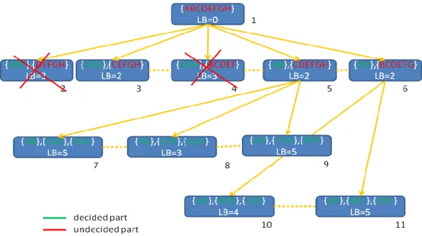
(36) Assume in the example, β is set at 3. The results from Phase 1 include two independent groups {A, B, C, D, E, F, G, H} and {J, K} in the partition. It means that each 2-itemset with one item from one group and the other item from the other group will be infrequent. However, the number of the first group {A, B, C, D, E, F, G, H} is eight, larger than the number threshold β. The group thus needs to be divided although it is an independent group as a whole. The group will be divided into 3 groups by the Refine-Partition procedure. The refining process will be shown later. Assume the procedure divide the group into three sub-groups {AB}, {CDF}, and {EGH}. The final partition is thus {{AB}, {CDF}, {EGH},{JK}} and the association relation between the parent group {A, B, C, D, E, F, G, H} in Phase 1 and its three sub-groups {AB}, {CDF}, and {EGH} are also kept for later mining. Next, the Refine-Partition procedure is explained. In the above example, the item number of the group {A, B, C, D, E, F, G, H} is bigger than β, and is thus a big group. It then needs to be refined into sub-groups by the proposed procedure, which is based on the branch-and-bound strategy. A search tree will be used to find the best refinement of the big group. It proceeds as follows. First, the upper bound of the whole solution space is set as an infinite value. Then the root node of the search tree is formed, with its decided part as null and its undecided part as the group {A, B, C, D, E, F, G, H}. The lower bound of the root node is initially set at 0. Then the child nodes are generated from the root node, each with one possible sub-group from the undecided part to the decided part. In this example, since there are 8 items in the group and the item number threshold is 3, each sub-group can then include 3 or 2 items. Besides, the sub-group must contain the first item {A} in the originally undecided part to avoid redundant checking. The results are shown in the top two levels of the search tree in Figure 3-1. 27.

(37) Figure 3-1: The search tree to divide a big group into small sub-groups. In Figure 3-1, all the subgroups with 3 and 2 items are enumerated based on the big group in the root node. Each sub-group must contain the item {A} and forms a child node. The low-bound of each child node is then calculated according to the proposed evaluation mechanism. Take the first node {{ABC}, {DEFGH}} as an example to show how to calculate the low-bound. In the example, {ABC} is in the decided part and {DEFGH} is in the undecided part. Table 3-4 shows the evaluation scores of all the 2-itemsets from the items in the big group. If a 2-itemset is infrequent, its score is 1; otherwise, it is 0.. 28.

(38) Table 3-4: All the 2-itemsets and their scores from the items in the big group 2-itemset. score. 2-itemset. score. 2-itemset. score. 2-itemset. score. AB. 0. BD. 0. CG. 1. EH. 1. AC. 0. BE. 1. CH. 0. FG. 1. AD. 0. BF. 0. DE. 1. FH. 1. AE. 1. BG. 1. DF. 0. GH. 1. AF. 0. BH. 1. DG. 1. AG. 1. CD. 0. DH. 1. AH. 1. CE. 1. EF. 1. BC. 0. CF. 0. EG. 1. The score of the decided part is first evaluated. It contains the subgroup {ABC}, which includes the three 2-itemsets AB, AC and BC. The score (Sdecide) of the decided part is then the summation of the individual scores, which is 0 + 0 + 0 (= 0) from Table 3-4. On the contrary, the undecided part contains {DEFGH}, which may be later divided into 2 sub-groups, respectively with 3 and 2 items. The number of 2-itemsets after it is divided will thus be C(3, 2) + C(2, 2), which is 4. The lower bound of the undecided part can then be set as the summation of the lowest four scores among the 2-itemsets generated from the undecided part, which are marked in underline in Table 3-4. Only one 2-itemset generated from the undecided part is with the score 0, and the others are with 1. Thus, the score (Sundecide) of the undecided part is 0 + 1 + 1 + 1, which is 3. The low-bound of the child node with {{ABC}, {DEFGH}} is then the summation of Sdecide and Sundecide, which is 0 + 3 (=3). All are the child nodes are then evaluated in this way. The unexplored node with the best lower bound is then chosen for search. In this example, the node with {{AB}, {CDEFGH}} has the minimum lower bound and will first be explored. 29.

(39) For the node {{AB}, {CDEFGH}} to be explored next, the undecided part is {CDEFGH}. It can then be further divided into two sub-groups with 3 items because the group in the decided part already contains two items. In this case, when one sub-group has been moved out from the undecided part to the decided part, the other sub-group has also been decided. Feasible solutions are thus generated at this level. Note the first sub-group to be moved out will contain the first item {C} in the undecided part for avoiding redundant checking. For example, a feasible solution generated from the above node is {{AB}, {CDF}, {EGH}} and the score is evaluated from the decided part since all the sub-groups are determined. The feasible solution has the best score (3) among all the unexplored nodes. Since it has been a possible refinement of the original big group and its score is larger than the original upper bound, which is infinite, it is then used as the new upper bound for the search. The nodes with their upper bounds equal to or larger than 3 are then pruned away. For example, the node {{ABC}, {DEFGH}} will be pruned since its lower bound is 3, equal to the upper bound. Next, the unexplored node {{AH}, {BCDEFG}} is searched since its lower bound is 2, smaller than the upper bound. Its child nodes were not better than the current best one and thus not the solutions. The same process is then repeated for the other unexplored nodes. For this example, the best refinement of the big group is {{AB}, {CDF}, {EGH}}. The final partition from the proposed algorithm is thus {AB}, {CDF}, {EGH}, and {JK}.. 30.

(40) CHAPTER 4 Item Partition by Genetic Algorithms 4.1 The Proposed Algorithm INPUT: 1.. A set of n transactions in a database with a set of m items {I1, I2, …, Im} named DIL (Domain Item List);. 2.. A minimum support threshold named min_support.. 3.. A number threshold β for constraining the number of items in each group of a partition.. OUTPUT: 1.. A proper partition P from the DIL with the item number in each group equal to or less than β.. 2.. The association relations between each big group and its refined sub-groups.. The proposed item-partition algorithm: PHASE 1: STEP 1: Generate all the 2-itemsets from the given items and calculate their counts. STEP 2: If the count of an itemset is larger than the threshold, min_support, then put it in the set of frequent 2-itemsets (FI). STEP 3: Initially set the partition P to have m groups, with each consisting of only one item in DIL. STEP 4: The two groups with the two items in a frequent 2-itemset will be merged 31.

(41) together if they belong to different groups for dependency consideration. STEP 5: Repeat the above step (STEP 4) until there is no frequent 2-itemsets or only one group in the partition. STEP 6: Output the partition into Phase 2 for possible finer division. PHASE 2: STEP 7: If in the partition there is at least one big group (with the item number larger than the number threshold β), do the next step; otherwise, exit the algorithm and output the partition. STEP 8: Use the “GA-based Refine-partition” procedure (shown later) to divide each big group into a set of small groups (with their item numbers equal to or smaller than β). STEP 9: Set the association relations between each big group and its refined sub-groups for the usage of later mining. STEP 10: Output the final partition and the association relations between each big group and its refined sub-groups.. Note that after step 10, a proper partition with no or little inter-group dependency can be found. The partition may then be used to improve the efficiency of data mining under some situations. For example, mining association rules under memory limitation is a good application of it. Next, the “GA-based Refine-partition” procedure, which divides each big group into a set of small groups, is introduced. It is stated as follows.. For each big group, the procedure first finds how many sub-groups are enough for it. It can be easily done by dividing the item number of the original group over the 32.

(42) item number threshold β and finding the ceiling of the result. This will cause the minimum number of sub-groups for the group. This is also what we desire since the sub-groups will depend on each other and the minimum number of subgroups can reduce the computation time for the later mining process. Then, the procedure will try to find the sub-groups with less inter-group dependency and with the item number of each equal to or less than the item number threshold β. The inter-group dependency is measured by the number of infrequent 2-itemsets in each group. It is a relative measure. That is, if the number of infrequent 2-itemsets in a group is small, then the number of frequent 2-itemsets is large and the group is much self-contained. Thus, the total of the numbers of the infrequent 2-itemsets in all the groups is used to measure the fitness of the partition. The minimum the value is, the better the partition. Since the total number of frequent 2-itemsets is known, it means that the number of inter-group 2-itemsets in this way is the minimum among all the possible partitions. Note that only 2-itemsets are used here to measure the goodness of a partition. Itemsets with more items can also be used to measure but they will raise the complexity of the real implementation and the computation time. The proposed GA-based partition refinement procedure is stated below.. The GA-Based Partition Refinement Procedure INPUT: A big group (with the item number larger than the number threshold β). OUTPUT: A set of small groups (with the item number equal to or larger than the number threshold β) with the minimum total of the numbers of the infrequent 2-itemsets in all the groups. The procedure is based on genetic algorithms. Some important details of the procedure are explained below. 33.

(43) Chromosome Representation It is important to design an appropriate chromosome representation for GAs to be applied. Several possible encoding approaches have been described in [3, 17, 21, 22]. Here, what we like to solve is to partition a big group into smaller sub-groups to satisfy the item number criterion. Assume the big group G to be divided consists of m items, represented as G = {I1, I2, …, Im}, where Ij is the j-th item in the group. Traditional integer coding schemes may generate infeasible solutions, thus needing extra checking time. For avoiding this, we design a new scheme, called partition transformation coding scheme, to assume all the offspring solutions generated by crossover or mutation operators are feasible. The proposed scheme is based on a hybrid scheme of binary and integer values. It is stated below. Assume the items in the initial big group are numbered according to their alphabet order. For example, assume the big group {A, B, C, D, E, F, G, H} are to be divided into smaller sub-groups. Their initial numbers are then encoded as 1 to 8, which remain unchanged in the whole GA process. They are called as the initial constant order of the items. Figure 4-1 shows the concept.. Figure 4-1: The initial constant order of the items in the example. For the partition refinement to satisfy the item number constraint in each group, the item number combination in the final resulting sub-groups may be known in advance. For consistency, the sub-groups with a smaller number of items are listed at front of those with a larger one. For example, assume the item number threshold is set at 3. The big group will thus be divided into 3 small sub-groups, with their item 34.

(44) numbers set at 2, 3, 3, respectively. The partition for the items with initial constant order in the big group is then formed according to the sequential numbers and the item numbers in the group. For the above example, A and B are in the first sub-group since their numbers are 1 and 2 and the group contains only two items. Similarly, C, D, E are in the second group, and F, G, H are in the third group. For the genetic process to be performed, a population composed of a set of chromosomes must be formed. As mentioned above, a new hybrid coding scheme is proposed, by which each chromosome consists of m+1 genes. Each of the first m genes corresponds to an item in the big group. The values of the first m genes are binary, with 0 or 1. The gene with the value 1 means its corresponding item has its original number. The gene with the value 0 means the number of its corresponding item will be shifted right for several steps, which are controlled by the last gene with an integer value. For example, 011001103 is a possible chromosome for the above example. The items A to H originally have their corresponding numbers 1 to 8, which are used to group them, as mentioned above. In the chromosome, the second gene is 1, which means the number of B is still 2. Similarly, the numbers of C, F, G are 3, 6, 7 since their corresponding gene values are 1. The numbers (1, 4, 5, 8) of the other items (A, D, E, H) will be shifted right for 3 times. Thus (4, 5, 8, 1) will be the new numbers for the four items. The numbers of the items from the chromosome is then (4, 2, 3, 5, 8, 6, 7, 1). The two items with the numbers 1 and 2 are B and H. They are then grouped together. The partition generated from the chromosome is then {B, H}, {A, C, D} and {E. F. G}. The process is shown in Figure 4-2.. 35.

(45) Figure 4-2: The transformation from a chromosome to a partition. From Figure 4-2, it can be easily observed that each chromosome can be transformed into a unique feasible partition from the binary values on itself with the aid of the initial constant order of the items. In implementation, a chromosome can be represented by an array c. Let length(c) represent the number of bits in the chromosome. Then length(c) = m +1, where m is the number of items to be processed. Let c[i] represent the i-th element in c. The first m bits of the chromosome thus represent the flags for whether the orders of the items are kept, and the last bit represents the sep number for order rotation. Formally, c[i] is defined as follows:.  0 or 1, if 1  i  lenngth (c)  1, c[i ]   Integer ( 0), if i  length (c).. In Table 4-1, we show the c array for the above example. In the example, length(c) is 9, the rotation value (last bit) is 3, the chromosome values for the items A, B, C, D, E, F, G, H, are 0, 0, 1, 0, 1, 0, 0, 0, 3.. 36.

(46) Table 4-1: An example for a chromosome. Item A B C D E F G H c[i] 0 0 1 0 1 0 0 0 3 Formally, the transformation process is stated in the following procedure.. The Chromosome Transformation Procedure: INPUT: A chromosome c with m+1 genes, the item number in each sub-group from the big group, and the initial constant order of the items. OUTPUT: A partition corresponding to the chromosome c. STEP 1: Set a temporary array shift to shift the order of the items with their corresponding genes being 0. STEP 2: Initially set a mapping array mapping as zero array, which will be used to keep the final mapping results from the chromosome c. STEP 3: If c[i] = 1, then mapping[i] = ICO[i], where c[i] is the i-th gene of the chromosome c and ICO is the initial constant order of the items, 1≦i≦m. STEP 4: If c[i] = 0, sequentially put ICO[i] in the array shift. STEP 5: Rotate right the array shift for c[m+1] positions. STEP 6: Sequentially put the contents in the array shift to the un-filled elements (with their corresponding genes = 0) of the array mapping. STEP 7: Group the items according to their numbers in the array of mapping with the aid of the known item number in each group.. After STEP 7, each chromosome can be uniquely mapped to a partition of the items. As it can be seen from the representation, each possible chromosome is feasible. 37.

(47) Take the data in Figure 4-3 as an example. Its processing is shown in Figure 4-3. The initial constant order (ICO) of the items in the group is (1, 2, 3, 4, 5, 6, 7, 8). The temporary array shift initially contains the four elements (1, 4, 5, 8) for the chromosome (0, 1, 1, 0, 0, 1, 1, 0, 3). It will be shifted right for 3 positions as {4, 5, 8, 1}. The array of mapping will thus become (4, 2, 3, 5, 8, 6, 7, 1). Assume the item number threshold is 3 in the example. The numbers of the three groups are thus 2, 3, 3, respectively. The first group is then {H, B} because their order numbers are 1 and 2. Similarly, the second and the third groups are {A, C, D} and {E, F, G}. The uniquely transformed partition for the chromosome (0, 1, 1, 0, 0, 1, 1, 0, 3) is then {{H, B}, {A, C, D}, {E, F, G}}.. Figure 4-3: The execution process of the transformation procedure. The Fitness Function The fitness value of a chromosome is the number of infrequent itemsets that are covered by the feasible solution represented by the chromosome. In the algorithm, the feasible solution with a smaller fitness value is better than that with a bigger value.. In the example, we assume the group ({{A, B, C, D, E, F, G, H}}) is divided as three groups ({A, B, C}, {D, E, F}, {G, H}). The group ({A, B, C}) can cover AB, 38.

(48) AC and BC, which are colored as red in Table 2. The group ({D, E, F}) can cover DE, DF and EF, which are colored as blue. The group ({G, H}) can cover GH, which is colored as green. The fitness value of the partition ({A, B, C}, {D, E, F}, {G, H}) is thus 3 because it covers 3 infrequent 2-itemsets.. Table 4-2: All infrequent 2-itemsets of group ({A, B, C, D, E, F, G, H}) 2-itemset. frequent. 2-itemset. frequent. 2-itemset. frequent. 2-itemset. frequent. AB. Yes. BD. Yes. CG. No. EH. No. AC. Yes. BE. Yes. CH. No. FG. No. AD. No. BF. No. DE. No. FH. No. AE. No. BG. No. DF. No. GH. No. AF. No. BH. No. DG. No. AG. Yes. CD. No. DH. Yes. AH. Yes. CE. Yes. EF. Yes. BC. Yes. CF. No. EG. No. The Crossover Operators Let the first chromosome be represented by the array c1, the second chromosome be represented by c2, the mask be represented by the array M, and the new chromosome be represented as the array cnew, which is the chromosome resulting from crossover of c1 and c2. Also let length(c1), length(cnew) and length(M) represent the number of elements of the chromosomes c1, cnew and M, respectively. length(DNA1)= length(DNA2)= length(DNAnew)= length(M). The i-th element of cnew can be represented as follows:. c [i ], if M [i ]  0, cnew[i ]   1 c2 [i ], if M [i ]  1.. 39.

(49) An example is shown in Table 3. cnew[i] represents the result from the crossover of c1[i] and c2[i]. In the example, cnew[1] = c2[1] = 1 because M[1] = 1, and cnew[2] = c1[2] = 0 because M[2] = 0. Table 4-3: An example for crossover c1[i]. 0. 0. 1. 1. 1. 0. 0. 1. 5. c2[i]. 1. 1. 1. 0. 0. 1. 1. 0. 4. M[i]. 1. 0. 0. 1. 1. 0. 0. 0. 0. cnew[i]. 1. 0. 1. 0. 0. 0. 0. 1. 5. The Mutation Operator Let a chromosome to be mutated be c, a mask be M, and the resulting chromosome be cmutation. Let length(c) and length(M) represent the number of elements in c and M, respectively. length(c) = length(M). The i-th element in cmutation can be represented as follows..  c[i], if M [i]  0 and 1  i  length (c)  1,  c[i], if M [i]  1 and 1  i  length (c)  1,  cmutation[i]   c[i], if M [i]  0 and i  length (c),  c[i]  arbitrary integer ( 0), if M [i]  1 and i  length (c).. An example is shown in Table 4. The value of cmutation[1] is changed to 1 because M[1] = 1, and the value of cmutation[2] is not changed because M[2] = 0. Table 4-4: An example for mutation c[i]. 0. 0. 1. 1. 1. 0. 0. 1. 5. M[i]. 1. 0. 0. 1. 1. 0. 0. 0. 0. cmutation[i]. 1. 0. 1. 0. 0. 0. 0. 1. 5. 40.

(50) CHAPTER 5 Generation of Frequent Itemsets from a Partition of Items 5.1 The Modified FP Tree In the past, many algorithms for mining association rules from transactions were proposed, most of which were based on the Apriori algorithm, which generated and tested candidate itemsets level-by–level. Han et al. proposed the Frequent-Pattern-tree (FP-tree) structure for efficiently mining association rules without generation of candidate itemsets. The FP-tree was used to compress a database into a tree structure which stored only large items. It was condensed and complete for finding all the frequent patterns. A recursive mining procedure called FP-Growth was executed to derive frequent patterns from the FP-tree. They showed the approach could have a better performance than the Apriori approach. In this paper, we slightly modify the FP-tree structure for effectively handling the cross-group mining problem. In the cross-group mining problem, items are partitioned into several groups and the mining process is first executed on each group to find individual itemsets. Since there may be some dependency among the items across the groups for mining, merging individual results is thus needed and is usually 41.

(51) complicated. Some additional information is then kept on the FP-tree to make the merging process easily. Here, the transaction numbers for each branch in the FP-tree is retained to achieve the purpose. The procedure for building the modified FP-tree (abbreviated as MFPT) is stated as follows. It is similar to the construction of an FPtree except for the consideration of group items and retaining of transaction IDs.. The MFPT construction procedure: Input: A data set D with n transactions with m items, a group of k items, and a user- defined minimum support (min_support). Output: The modified FP-tree (MFPT). STEP 1: Generate an initial MFPT with only the empty root node. STEP 2: Set the initial count of each item in the given group as 0. STEP 3: Sequentially read a transaction from the given data set D and delete the items that does not appear in G. STEP 4: If an item in G appears in the transaction, add its count by 1. STEP 5: Repeat STEPs 3 and 4 until all the transactions are processed. STEP 6: Compare the items with min_support and remove the items which are not frequent. STEP 7: Sort the items in G according to their final counts. 42.

(52) STEP 8: Sequentially read a transaction T from the given data set D. STEP 9: Generate a tree path P from the transaction T with only the frequent items according to the sorted order in STEP 7. Merge P into MFPT in a way similar to FPT. STEP 10: Add the count of each node in P of MFPT by 1 and add the transaction ID (TID) of T to the last node of P. STEP 11: Repeat STEPs 8 to 10 until all transactions in D are processed.. After STEP 11, the modified FP-tree is built. Below an example is given to show the difference and the procedure for building the modified FP-tree.. Example 1: Assume the 10 transactions shown in Table 1 are used as the data set. In Table 5-1, the domain of the transaction database includes 10 items (A to J). Table 5-1: The transaction data set used as the example TID. Items. TID. Items. 01. A, B, C, D, F, G. 06. B, C, D, E, F, H. 02. B, C, D, G, H, I. 07. C, F, G, H. 03. A, B, D, E, F, G. 08. A, B, C, D, F, H. 04. B, D, E, G, H. 09. A, B, C, F, J. 05. A, B, E, F, I. 10. B, C, D, F, J. Also assume the group to be processed contains only the three items {A, B, D}. 43.

(53) The procedure proceeds as follows. First, The counts of the three items {C, F, G} are initially set as 0. The first transaction in the transaction data set is read, which is composed of the six items, {A, B, C, D, F, G}. The items C, F, and G are removed and not processed because they are not in the group. The count of the three items {A, B, D} are thus added by 1. Then the other transactions are processed one by one by the same process. At last, the counts of the three items are 6, 9, 6, respectively. The three items are then sorted as the order of B, A, D. Then the first transaction is scanned again to build the first branch (B, A, D) of the tree according to the sorted order as shown in Figure 5-1. The Transaction ID for the branch is also put in the last node.. Figure 5-1: The MFPT after the first transaction is processed. The second transaction is then processed. Its content is {B, C, D, G, H, I}. The above procedure will generate the path (B, D) and merge it with the previous MFPT. The MFPT after this transaction is processed is shown in Figure 5-2.. 44.

(54) Figure 5-2: The MFPT after the second transaction is processed. Next, the third transaction is processed. Its content is {A, B, D, E, F, G}. The above procedure will generate the path (B, A, D) and merge it with the previous MFPT. The transaction ID (03) for the path will be put in the node D of the path (B, A, D) in the MFPT. The resulting MFPT is shown in Figure 5-3.. Figure 5-3: The MFPT after the third transaction is processed. Continuing the same procedure for the other transactions, the final MFPT after all the ten transactions are processed for the group of items {A, B, D} is shown in Figure 5-4. 45.

(55) Figure 5-4: The final MFPT. Note that the FPT for the item {A, B, D} is also shown in Figure 5-5 for a comparison. As you can see from Figures 5-4 and 5-5, the main difference of the two trees lies in the transaction IDs in the nodes. These transactions IDs will be used to help find cross-group itemsets effectively and efficiently.. Figure 5-5: The final FPT for a comparison. 46.

(56) 5.2 The Enumeration Tree The modified FP-Growth mining process is then executed on the MFPT to get the frequent itemsets in a recursive way. It will generate the conditional modified FP trees and find out the frequent itemsets from the conditional trees in a similar way to FP-Growth. However, in generating the frequent itemsets, the transactions belong to each frequent one can be easily found with the aid of keeping corresponding transactions IDs in the nodes of MFPT. Besides, the recursive process of the modified FP-Growth procedure will check the itemsets in an enumerated order of the frequent items in G. For the above example, its enumerated order will be (B, BA, BAD, A, AD, D). The order can be presented by the enumeration tree as shown in Figure 5-6. All the itemsets in the enumerated tree are generated by the items B, A and D. The transaction IDs belonging to each itemset can also be easily obtained with the aid of the MFPT and are also shown in the enumeration tree.. Figure 5-6:The enumeration tree for representing the execution order of the modified FP-Growth procedure. 47.

(57) In Figure 5-6, the content of each node contains an itemset and its corresponding transaction numbers. For example, the node {BA}(01, 03, 05, 08, 09) means that the transactions IDs of the itemset {BA} are 01, 03, 05, 08 and 09. In the actual implementation, the tree may be not complete because of the downward-closure property. That is, when the frequent itemset represented by a node in the tree is not frequent, its child nodes will not be frequent also and don’t need to be enumerated in the tree. Assume the minimum support value is 5. The pruned enumeration tree is shown in Figure 5-7.. Figure 5-7: The pruned enumeration tree. An enumeration tree has the following properties. 1.. The itemset in a node must be the superset in its parent node. The also means that the transaction IDs in a node must be included in the transactions IDs in its parent node.. 2.. The item number of a node is the item number of its parent node plus 1.. 3.. The item that appears in a node and does not appear in its parent node is put at 48.

(58) the most right side of the items in the node.. 5.3 Compacted Frequent Itemsets As mentioned before, Figure 5-6 shows all the frequent itemsets and transaction IDs in the enumeration tree. Usually in real applications, the item numbers are very large, and thus the memory space for storing an enumeration tree may also be very large as well. In order to reduce the memory space, we use the above properties of an enumeration tree to compact the contents of the tree. The method is explained below. First, each path in the pruned enumeration tree is identified. It has the property that an itemset in a path cannot be in another path. Besides, according to the properties of an enumerated tree, the itemset at the leaf node of a path is the superset of the other itemsets in the same path. For example, in the path of {B} -> {BA} -> {BAD}, the itemset of {BA} can be obtained by deletion of the most right item from the leaf node {BAD}, and the itemset of {B} can be obtained by deletion of the most right two items from the leaf node. Besides in an enumeration tree, the transaction IDs in a node must be included in the transactions IDs in its parent node. According to the property, we may represent path information from the viewpoint of transaction IDs. That is, for each path, the number of itemsets appearing in a transaction may be counted and kept. For the above 49.

(59) example, the information in the path {B} -> {BA} -> {BAD} can be summarized as {01: 3, 02: 1, 03: 3, 04: 1, 05: 2, 06: 1, 08: 3, 09: 2, 10: 1}, where the first number in each item is a transaction ID and the second number is the itemset number. For example, the information “01: 3” means that three itemsets appear in the first transaction in the path. The list is thus called the appearing count list and abbreviated ACL. The transactions for the itemset BAD at the leaf node of the path can then be easily known as (01, 03, 08) from the above summary information with the itemset number of a transaction equal to the item number of BAD, which is 3 in the case. Similarly, the itemset number for BA is 2 and for A is 1 since the itemset BAD includes BA and BA includes B. The transaction IDs for BA and B are thus found to be {01, 03, 05, 09} and {01, 02, 03, 04, 05, 06, 08, 09, 10}, respectively. The itemset in a leaf node of a path with the above information is then called a compact frequent itemset, abbreviated as CFI. A CFI can then represent a path in an enumeration tree. It consists of a leaf frequent itemset (LFI) of a path in the enumeration tree and an appearing count list (ACL). All the CFIs gathered together can represent the enumeration tree. In other words, an enumeration tree can be completely reconstructed from the kept CFIs. Figure 5-8 shows all the CFIs obtained from the enumeration tree in Figure 5-6.. 50.

(60) Figure 5 8: All the CFIs from the enumeration tree in Figure 5-6. Formally, the construction process of CFIs from an enumeration tree is stated as follows. It can be executed together when FP-Growth finds all the frequent itemsets that are in a path of the enumeration tree.. The construction process of CFIs from an enumeration tree: INPUT: A path of frequent itemsets FI generated by the modified FP-Growth approach, each of which has its known covered transaction IDs. OUTPUT: A CFI corresponding to the given itemsets. STEP 1: Initially set the appearing count list (ACL) as an empty list. STEP 2: Find the leaf frequent itemset LFI that has the maximum number k of items in FI. STEP 3: Put (LFI, ACL) to CFI. STEP 4: If k-1 > 0, then do the next step; otherwise go to STEP 9. 51.

(61) STEP 5: For each transaction covering LFI, which can be known from input, form the pair (transaction ID, 1) and put the pair to ACL. STEP 6: Find the next frequent itemset NFI that has k-1 items in FI. STEP 7: For each transaction covering NFI, which can be known from input, form the pair (transaction ID, 1) and append it to ACL if the transaction has not been in ACL yet, and increase the itemset value of the transaction by 1 if the transaction has been in ACL. STEP 8: Set k = k – 1 and go to STEP 4. STEP 9: Output CFI.. After STEP 9, the CFI corresponding to the given path of itemsets are generated. Note that in the procedure, the input includes the transaction IDs for an itemset to appear. They can be easily found through the following Transaction-IDs-Search procedure.. The Transaction-IDs-Search Procedure: INPUT: A MFPT , an itemset IS in it and the sorted list of items according to the counts (which may be generated when the MFPT is constructed). OUTPUT: The set of transactions IDs in which the itemset IS appears. 52.