全流域數值模型研發及其在淹水改善檢討之應用─以大台北都會區淹水改善檢討為例－總計畫暨子計畫:洪汛期間水庫操作規線上限對河川洪水位之影響(I)

行政院國家科學委員會專題研究計畫 成果報告

全流域數值模型研發及其在淹水改善檢討之應用─以大台

北都會區淹水改善檢討為例--總計畫暨子計畫:洪汛期間水

庫操作規線上限對河川洪水位之影響(I)

研究成果報告(完整版)

計 畫 類 別 ： 整合型 計 畫 編 號 ： NSC 95-2625-Z-002-018- 執 行 期 間 ： 95 年 08 月 01 日至 96 年 07 月 31 日 執 行 單 位 ： 國立臺灣大學土木工程學系暨研究所 計 畫 主 持 人 ： 徐年盛 共 同 主 持 人 ： 鄭昌奇、簡振和 計畫參與人員： 博士後研究：魏志強 處 理 方 式 ： 本計畫可公開查詢

中 華 民 國 96 年 09 月 29 日

洪汛期間水庫操作規線上限對河川洪水位之影響（I）

Effect of Flood Control Curve On River Stage During Flood Period (I)

摘

要

本研究第一年建立一多水庫防洪最佳即時操作模式以供水庫在颱洪來臨時據以運轉水庫及降 低洪災之用。多水庫防洪最佳即時操作模式之目標函數包括：(1)降低下游控制點之洪峰流量最大 化；以及(2)滿足洪水過後水庫蓄水量最大化。模式限制式採納適用於台灣水庫短期距防洪之三階 段放水原則。本研究以淡水河流域為範例，結果顯示多水庫防洪最佳即時操作模式可較歷史營運記 錄及防洪放水規則操作更有效地降低洪峰並達到洪峰後蓄水目標，由此彰顯了模式之應用性。 關鍵詞：防洪即時最佳操作，優選模式，水庫放水

Abstract

Effect of flood control curve to river stage during flood period is estimated by a multireservoir optimization model for basin-scale flood control at the first year. In order to determine the optimal hourly releases from reservoirs under the estuary tidal effects during typhoon periods, this paper develops a generalized multipurpose multireservoir optimization model for basin-scale flood control. The model objectives include: reducing the downstream floodwaters, and meeting reservoir target storage at the end of flood. The model constraints include the reservoir operations and the neural-based linear channel level routing. The proposed channel level routing based on feed-forward back-propagation neural network is used to estimate the downstream water levels. The developed optimization model has been applied to the Tanshui River Basin system in Taiwan. The results of optimization model running, in contrast to historical records, successfully demonstrate the practicability in solving the problem of flood control operations.

1. Introduction

Tanshui River Basin is located in the northern part of Taiwan having steep terrain and excessive rainfall. The most severe disaster in Tanshui River Basin is flooding which is caused by the intensive rainfall and rapid flows during typhoon seasons. Once typhoon strikes, the water level at the estuary rises abnormally by typhoon surge. Meanwhile, receiving voluminous rainfalls from upstream watershed, considerable streamflows usually converge downstream in a short time. Therefore, it is very difficult to release such voluminous water into ocean for the downstream reach. With all these unfavorable natural conditions, multireservoir operations play an important role in mitigating the downstream flood disaster.

For developing a multireservoir operation model for a river basin system, Windsor (1973), Needham

et al. (2000), and Braga and Barbosa (2001) described an application of deterministic optimization using

a linear programming (LP) model to treat the flood control problem, using the Muskingum method for channel routing and mass balance equation for reservoir operations. Wasimi and Kitanidis (1983) applied the discrete-time linear quadratic Gaussian (LQG) stochastic control for the real-time daily operation under flood conditions. The streamflow routing along a channel reach used the Muskingum linear channel routing model. Unver and Mays (1990) formulated a nonlinear programming (NLP) model to address the real-time hourly flood control problem. The constraints included the reservoir operation constraints, which are defined by bounds on reservoir releases, surface elevations and gate facilities; the hydraulic constraints are defined by the one-dimensional unsteady flow. The above published papers have studied the multireservoir operation problem well. However, such case with tidal effects by typhoon surge has not been studied in the past.

For solving the complicated flow routing under the interaction between upstream flows and tidal effects, Lai (1986; 1999; 2002) developed a CCCMMOC model, which is one of the gradually varying unsteady flow methods. In the last two decades, he has succeeded in applying a model for simulating the complicated behavior of water movement and interaction at each river section in Tanshui River (Lai, 2002). The CCCMMOC model demonstrates that it is good at accurately analyzing the variations of water surface elevation under the unsteady channel flow. In the CCCMMOC model, however, the multireservoir operations have not been taken into consideration. Moreover, the time consumed for computer calculation makes it inefficient.

Artificial neural networks (ANN) are good at identifying and learning correlated patterns between input data sets and the corresponding target values (Chang and Chen, 2001; Huang, 2001). After McCulloch and Pitts (1943) established the first neural network, a number of ANNs were developed to solve different problems such as water level predictions (e.g., Bazartseren et al., 2003; Chang and Chen, 2003; Tissot et al., 2004). This study proposes a neural-based linear channel level routing algorithm based on feed-forward back-propagation neural network (BPNN) to estimate the downstream water level.

The purpose of this paper is to formulate a generalized multipurpose multireservoir optimization model for basin-scale flood control to determine the optimal hourly releases under tidal effects. The presented optimization model is formulated as a mixed-integer linear programming (MILP) model. The model constraints include the reservoir operation rules and the neural-based linear channel level routing.

The developed optimization model will apply to the Tanshui River Basin system in Taiwan.

2. Tanshui River Basin System

2.1. SYSTEM DESCRIPTION

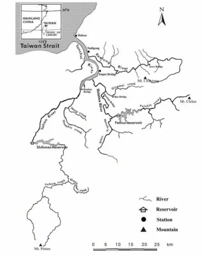
Figure 1 shows the geographical location of the greater Tanshui River Basin. The Tanshui River consists of three major river basins: Tahan River, Hsintien River, and Keelung River. The major stream flows of Tanshui River go through the Taipei Bridge and Tudigong, and finally reach Hekou. In this basin, the parallel Shihmen and Feitsui Reservoirs, have been used for joint operations for flood control.

Tahan River originates from Mt. Pinten and joins the Hsintien River at Chiangchutsui, which is the starting point of Tanshui River. The length of Tahan River is 126 km with a drainage area of 1,163 km2. There are four major creeks in the Tanhan River, including Yufong creek, Shankwan creek, Shanshia creek, and Heng creek. The Shihmen Reservoir, completed in 1964, is the most important hydraulic structure in the Tahan River. The maximum elevation of 245 m is for normal operation, whereas the maximum elevation of 248 m is for flood-mitigation operation. Approximately the capacity of 27 106 m3 is reserved for flood control during typhoon invasions. The Shihmen Reservoir currently managed by the Water Resources Agency was built primarily for flood control and the water is used for the irrigation and domestic water supply along the Tanhan River (Hsu and Cheng, 2002).

Hsintien River originates from Mt. Chilan and joins Tanshui River at Chiangchutsui. The length of Hsintien River is 82 km, with a drainage area of 916 km2. There are three major creeks in the Hsintien River, including Peishih creek, Nanshih creek, and Gingmei creek. The Feitsui Reservoir, completed in 1985, is the most important hydraulic structure in the Hsintien River. The maximum elevation of 170 m is for normal operation and the maximum elevation of 171 m is for flood-mitigation operation. Approximately 9 106 m3 of the storage is reserved for flood control during the typhoon season. The Feitsui Reservoir currently managed by the Taipei City Government was built primarily to provide domestic water supply to the Taipei Metropolitan area (Hsu and Cheng, 2002).

2.2. NETWORK REPRESENTATION

For the easy representation of a complex study area, the network representation (see Figure 2) is used. In Figure 2, nodes are introduced to represent reservoirs, control points, and the estuary; arcs are used to represent rivers. In this study, the two gauge stations (i.e., Taipei Bridge and Tudigong, locations are shown in Figure 1) are selected as control points. Table I lists the denotations of nodes and arcs.

3. Optimization Model

The proposed linear optimization model requires all relations associated with objective functions and constraints to be linear or linearized representations. The proposed optimization model can be described in detail as in the following.

3.1. CONSTRAINTS

The model constraints involve two parts: (1) the multipurpose multireservoir operations for flood control, and (2) the control-point level routing by using neural-based linear channel level routing algorithm. The configuration of Part 1 and Part 2 can be seen in Figure 2.

For the Multireservoir system operations (Part 1), the constraints include reservoir continuity and physical limitations. In addition, in view of implementing the reservoir flood operations in Taiwan, the flood control polices (rules) are embedded into constraints.

 Reservoir continuity: The constraints associated with a reservoir node (see Figure 2) for continuity of mass in inflowI_{i t,} , outflow R_,

i t

X , and storage S_, i t

X can be expressed according to the finite difference

formula



, 1 ,





, 1 ,



, , 1 , [ , ]0 2 2 R R S S i t i t i t i t i t i t t t I _ I X _ X X X _ i t t T          (1)

where i is the index of reservoir; t is the index of time period; t is a short time interval in hours for routing;  is the set of reservoirs; T is the flood duration; and t0 is the operating initial time. The

whole control horizon is the time length between t0and T. It is noticed that when t is equal to t0, both

the reservoir initial release

0 , 1

R i t

X _ (can be denoted asR_i,0) and storage

0 , 1 S i t X _ (denoted asS_i,0) are known.

 Physical limitations: The reservoir storage ranges from full storage ( max

i

S ) to dead storage (Sidead) over the control horizon, that is

dead max

, , [ , ]0

S

i i t i

S X S i t t T (2) In addition, for reservoir outflow capacity, the outflow amounts based on hydraulic facilities by employing linearized representations are limited. It can be achieved in four steps (Needham et al., 2000):

Step 1: Dividing storage. The whole reservoir storage volume is divided into zones (e.g., three zones in Figure 3). Hence, the total storage ( S_,

i t

X ) can be the sum of storage ( S_,l

i t X ) in these divided zones, that is , , 0 , , [ , ] l S S i t i t l l X X i t t T  



  (3)

where l is the index of storage zone, and  is the set of storage zones. Step 2: Limiting storage zone. The storage in each zone is constrained as

max , , , , [ , ]0 l S i t l i X S i  l t t T (4) where max , l i

S is the maximum value of storage zone l in reservoir i.

reservoir storage. The restricted release can be specified as





, , , 1 , 0 , 0 , [ , ] 2 l l S S R l i i t i t i t l l m X X _ X i t t T   



   (5)

where ml i, is the slope of the storage-release capacity relationship at storage zone l in

reservoir i.

Step 4: Correcting the release logic. To correctly represent release logic, for example, storage zones 1 and 2 are filled before water is stored in zone 3. The following binary variable ( ) andi t,

logical constraints must be added for each reservoir i.

3 2 2 max , , , 1 1 , 0 max , , 3, {0,1}, , [ , ] l S i t i t l i l l i t S i t i t i X S i t t T X S         _        _





(6)

 Operation rules: The reservoir flood control rules stipulate the release operation rules in Taiwan in order to mitigate flood damage (Water Resources Agency, 2002; Taipei City Government, 2004). A summary of release rules regarding the two flood stages and the corresponding constraints are described as follows.

For the peak-flow-preceding stage, there are two rules in this stage: Rule 1, that is, the reservoir release is less than or equal to the reservoir inflow; Rule 2, that is, the release at current period is greater than that at the previous period. Rule 1 and Rule 2 can be integrated into an equation

, 1 , , , [ , ]0

R R

i t i t i t a

X _ X I i t t t (7) where t_a is the ending time of the peak-flow-preceding stage when reservoir peak inflow occurs.

For the peak-flow-proceeding stage, there are two rules: Rule 1, that is, the release at each period is less than the reservoir peak inflow; Rule 2, that is, the release at the current period is less than that at the previous period. Rule 1 and Rule 2 can be integrated as follows:

peak

, , 1 , [ 1, ]

R R

i t i t i a

X X _I i  t t T (8)

where I_ipeak is the peak inflow at reservoir i.

For the downstream flood movement (Part 2), this study proposes a neural-based linear channel level routing algorithm. Figure 4 is a schematic of a typical BPNN with a three layer (i.e., an input layer, a hidden layer, and an output layer). Mathematically, a three-layer BPNN with N1 input nodes, N2 hidden

nodes, and N3output nodes, can be expressed as (Xu and Li, 2002)

2 1 2 1 2 1 3 0 0 [1, ] N N r qr pq p q p y f w f w x r N       _  _  _    





 (9)

the weight set connecting input layer and hidden layer; wqr2 is the weight set connecting hidden layer and

output layer; yr is the outputs from the network; f1



is the activity function on the hidden layer;

and f2



is the activity function on the output layer.

The bias weights and terms appear when p or q equals 0. The commonly used activity function includes linear, sigmoid and hyperbolic tangent (Imrie et al., 2000; Xu and Li, 2002). This study introduces the linear activity function for this algorithm. Thus, Eq. (9) can be rewritten as

2 1 2 1 3 0 0 [1, ] N N r qr pq p q p y w w x r N   



   (10)

As in Figure 4, the input layer can be used to receive the hydrological time series information including the reservoir releases, tributary and lateral runoffs, estuary levels, control-point levels, time delay, and so on; and the output layer is to output the control-point water level. From Eq. (10), the formula of the linear channel level routing can be expressed as

3 1 2 1 1 2 2 3 3 1 2 3 1 2 3 tribu , 1, 2, 1 1 1 W W W L R R k t kd t d kd t d kd t d d d d X X X I          



 



 



 5 6 4 4 4 5 5 6 6 4 5 6 4 local 5 mouth 6 , 1 1 1 W_{kd t d} W_{kd t d} W_{kd k t d}L d d d I L X k          



 



 



  (11)

where k is the index of control points;  is the set of control points (i.e., Control-point 1 and Control-point 2);d₁ d are indices of lag-time;₆ ₁ are lengths of lag-time associated with the related₆

hydrological information; and

1 1

Wkd ₆

6

Wkd are the weighting parameters. The seven terms of Eq. (11) are defined as follows.

,

L k t

X = variable associated with the water level elevation at Control-point k at time t, k{1, 2};

1 1,

R t d

X _ = variable associated with the release of Reservoir 1 at lag-time d1;

2 2,

R t d

X _ = variable associated with the release of Reservoir 2 at lag-time d2;

3 tribu

t d

I _ = flow of the Tributary at lag-time d3;

4 local

t d

I _ = flow of the total amount of Lateral 1, Lateral 2, and Lateral 3 at lag-time d4;

5 mouth

t d

L_ = water level elevation at Estuary at lag-time d5;

6 ,

L k t d

3.2. OBJECTIVE FUNCTION

In this study, for a multipurpose multireservoir operating system taking into consideration of controlling flood and regulating storage, the model objectives include (1) maintaining reservoir safety, (2) mitigating downstream flood hazard, and (3) meeting target reservoir storage at the flood ending. Mathematically, the objective function can be formulated as

, , , Min RP EP LP i i k i i i i k k X X X          







 (12) where RP i

X is the maximal release at reservoir i; EP

i

X is the maximal target storage error that is the

difference between storage and target value (i.e.,Sitarget, the target storage in normal periods at reservoir i);

and LP

k

X is the maximal water level at Control-point k.  The first objective (i.e.,

, Min RP i i i X 



) is to minimize the maximal reservoir release. For a min-max problem, it should be subjected to

, , [ , ]0 P R R i t i X X i t t T (13)  The second objective (i.e.,

, Min EP i i i X 



) is to minimize the maximal target storage error during the specific time interval at the flood ending periods. Thus, the min-max problem is subjected to

target , , [ , ] P P E S E i i t i i b X X S X i t t T       (14)

where tb is the starting time for regulating storage. It is noted that ta   .tb T  The third objective (i.e.,

, Min LP k k k X 



) is to minimize the maximal water level at the selected control points during flood. Similarly, the min-max problem is subjected to

, , [ , ]0 P L L k t k X X k t t T (15) The above objective function is used to explicate the trade-offs between the three objectives. However, there exists a problem with different scales among these objectives. Therefore, this study uses the dimensionless method to tackle the problem. Thus Eq. (12) can be rewritten as

peak target bank , , , Min P P P R E L i i k i i i i i i k k k X X X I S L          







 (16)

where Lbankk is the elevation of embankment at Control-point k.

Prior to application of the proposed model, this section concentrates on the parameters setup and weights calibrating.

4.1. PARAMETERS SETUP

For the Tanshui River Basin system, the reservoir characteristics are listed in Table II. Currently, the embankment elevations of Control-points 1 and 2 are at the altitude of 10.0 m and 4.8 m, respectively. The setup of time phases regarding the peak-flow-preceding stage and the peak-flow-proceeding stage are defined as:

 For Reservoir 1: Based upon Water Resources Agency (2002), the initial operating time t0 is at 600

m3/s inflow. In addition, this study assumes that the starting regulating storage time tb is at 400 m3/s inflow and the flood ending time T is at 300 m3/s inflow.

 For Reservoir 2: Based upon Taipei City Government (2004), the initial operating time t0 is at 500

m3/s inflow. Also, both the starting regulating storage time tbat 150 m3/s inflow and the flood ending time T at 100 m3/s inflow are supposed.

In order to choose the suitable lag-time lengths from various hydrological sources of the channel level routing, for simplicity, the travel time caused by propagating flood wave from a source point to the specific control point has been regarded as the lag-time length. For example, empirically, the travel time (1) of reservoir release from Reservoir 1 to Control-point 2 takes four hours roughly when flood occurs.

Table III lists all the lag-time lengths based upon the similar empirical way.

4.2. CHANNEL LEVEL ROUTING VALIDATION

In this section, the weights within the neural-based linear channel level routing formula (i.e., Eq. (11)) are first calibrated. Then, the linear channel level routing is compared to CCCMMOC model running.

For training the weights, the collected data for 36 typhoons (1987–2004), published by the Water Resources Agency, are divided into two independent subsets: the training and validating subsets. The training subset includes 26 typhoons (1,564 hourly records) and the validating subset has 10 typhoons (620 hourly records). Based on normalized data, two weight sets by BPNN are trained with the following parameters:

 For Control-point 1: The input nodes = 11, hidden nodes = 8, output node = 1, training cycles = 8,000, learning rate = 2.0, and momentum = 0.5. The BPNN is trained using the BFGS Quasi-Newton

algorithm as implemented within the software Matlab.

 For Control-point 2: The input nodes = 14, hidden nodes = 10, output node = 1, and other parameters are the same as Control-point 1.

The performance is assessed based on the criterion of root mean square error (RMSE), that is



_{sim obs}



2 1 ( ) ( ) RMSE= N j L j L j N  



(17) where sim ( )

L j is the simulated water level at record j; obs

( )

and N is the number of hourly records.

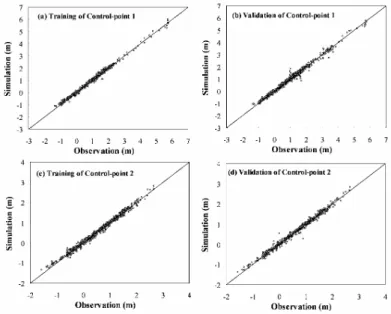
During the training processes, the weights gradually converge to values in which input vectors produce output values as close as possible to the target output desired. The results show that: (1) for Control-point 1, the RMSE of training = 0.020 and validation = 0.027; and (2) for Control-point 2, the RMSE of training = 0.015 and validation = 0.018. Figure 5 depicts the scatter plots of observation vs. simulation of the training and validation. By means of weights calibration, the linear channel level routing formulas at the two control points are obtained.

Prior to comparisons, the CCCMMOC model is briefly introduced. As mentioned in Section 1, CCCMMOC model is a powerful model for the simulation of riverine flow. The feature of the CCCMMOC model is to deal with the Compound-Complex Channel (network or dendritic) system based on the Multimode Method of Characteristics. Essentially, the governing equations of this one-dimensional model are based on Saint-Venant equations, which consist of the two following partial differential equations (i.e., continuity and motion) (Lai, 1986):

h Q B q t x       (18)



b f



Q Q Q Q h Q gA gA S S qu t A x x A x  _  _  _  _{   }     _{ }  (19)

where B is the width of the river cross-section; h is the flow depth (i.e., the elevation difference between water surface and channel bottom); Q is the river flow; q is the lateral flow per unit length; A is the cross-sectional area; g is the acceleration of gravity; Sbis the bed slope of channel; Sf is the slope of the energy gradient; and uis the lateral flow velocity in the x-direction. In order to solve this problem, Lai developed the multimode method of characteristics for multiple-reach rivers and estuaries. The details can be found in Lai (1965; 1986; 1988).

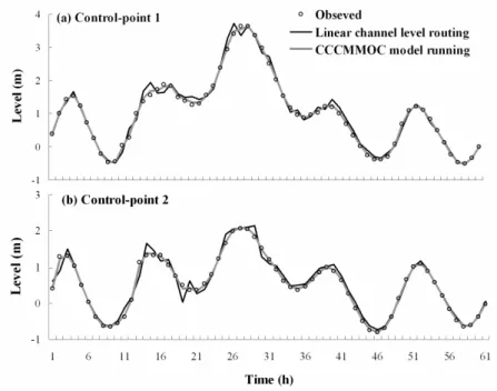
In here, the CCCMMOC model is used in the Tanshui River system which is divided into 17 reaches. Each reach corresponds to a resistance coefficient which was calibrated and verified by Lai (1999). The Hsinhai Bridge, Showlan Bridge, Bao Bridge and Tawa Bridge (the locations see Figure 1) are used as the upstream boundaries, and Hekou is the only downstream boundary. Typhoon Xangsane in 2000 is used for simulating the water level variations at Control-point 1 and Control-point 2. Figure 6 shows the simulation results of CCCMMOC model as well as the neural-based linear channel level routing. In comparison, the results of the linear channel level routing are slightly less accurate than the CCCMMOC model. However, the neural-based linear channel level routing demonstrates that it still is a good alternative method.

5. Application

Typhoons Aere in 2004 and Nari in 2001 are first selected for applying the proposed optimization model. Both typhoons were unusually extreme typhoons in recent years in Taiwan. Table IV, Figures 7 and 8 display the related hydrological characteristics of the two typhoons in Tanshui River Basin system. Typhoon Aere contains a single peak event in the two reservoir inflow hydrographs (see Figure 7a-b) while typhoon Nari has two peak events (see Figure 8a-b).

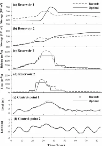
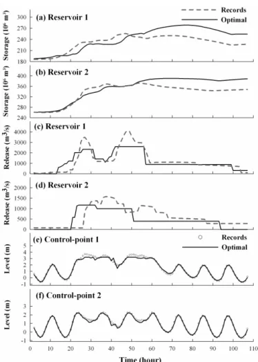
solving linear, nonlinear, and integer programming problems. LINGO uses the branch-and-bound algorithm to deal with the integer variables (LINGO, 2001). The computing time of each typhoon case with a Pentium M 1.70 GHz processor is 70 seconds approximately. Comparisons are made between the records and optimization model running. Figures 9 and 10 respectively show the results of typhoons Aere and Nari with respect to the reservoir storage and release hydrographs as well as the control-point level hydrographs.

From Figures 9c-d and 10c-d, one can see that the maximal releases of Reservoirs 1 and 2 in the two typhoons derived from optimization model are less than that historic operation records. In Figures 9e-f and 10e-f, the model results of the maximal levels of Control-points 1 and 2 exhibit more positive than records in reducing the downstream floodwaters. Also, for meeting reservoir target storage at the end of flood, Figures 9a-b and 10a-b show that the results derived from model can be carried out in Reservoirs 1 and 2.

It should be pointed out that for the water level at Control-point 2 in typhoons Aere and Nari (see Figures 9f and 10f), the difference between records and optimal values are limited. The reason is because Control-point 2 (i.e., Tudigong station) is close to the estuary in which it leads to the influence of tide much greater than that of upstream floodwater movement.

Additionally, this paper analyzes other four typhoons, including Herb of 1996, Zeb of 1998, Xangsane of 2000, and Haima of 2004 (the hydrological characteristics see Table IV). In order to assess the performance of the optimization model, several criteria are taken into account, defined as follows.

 Reservoir maximal release reduction rate (RR)

peak max peak RR(%) I R 100 I    (20)

where Ipeak is the reservoir peak inflow, and Rmax is the reservoir maximal release.  Reservoir target storage meeting rate (TM)

end target TM(%) S 100 S   (21) where end

S is the reservoir storage at the end of flood, and target

S is the target storage in normal periods.

 Control-point maximum level reduction rate (LR)

max LR(%) L L 100 L      (22) where max

L is the control-point maximal level during flood, and Lis the control-point maximal level based upon supposing no building upstream reservoir. The Lcan be derived from linear channel level routing (i.e., Eq. (11)) by substituting reservoir inflows for reservoir releases.

Generally, the higher the criterion is, the greater the performance is. Figure 11 shows that the bar charts concerning the performance of optimization model and records in six typhoons. Clearly, the results of the proposed model are better than records.

This paper develops a multipurpose multireservoir optimization model for basin-scale flood control. The optimization model is used to determine the reservoir releases. The model objectives include: preventing reservoir dam from overflow, reducing the downstream floodwaters, and meeting reservoir target storage at the flood ending. The model constraints include reservoir multipurpose flood control operation and channel routing under tidal effects. The optimization model is formulated as a mixed-integer linear programming (MILP) model. In order to formulate a linear channel level routing, the proposed neural-based linear channel level routing algorithm demonstrates a good alternative method in comparison with CCCMMOC model.

The developed model has been applied to the Tanshui River Basin system in Taiwan by using the observed hydrological data of six typhoons. The optimization model successfully demonstrates its practicability for the problem of multipurpose multireservoir flood control under tidal effects in contrast to records. For future studies, this paper suggests that the presented generalized optimization model can be used in real-time flood control operations to identify the multireservoir real-time releases at each flood period.

References

Bazartseren, B., Hildebrandt, G., and Holz, K. P., 2003, ‘Short-term water level prediction using neural networks and neuro-fuzzy approach’, Neurocomputing 55, 439–450.

Braga, B., and Barbosa, P. S. F., 2001, ‘Multiobjective real-time reservoir operation with a network flow algorithm’, Journal of the American Water Resources Association 37(4), 837–852.

Chang, F.-J., and Chen, Y.-C., 2001, ‘A counterpropagation fuzzy-neural network modeling approach to real time streamflow prediction’, Journal of Hydrology 245, 153–164.

Chang, F.-J., and Chen, Y.-C., 2003, ‘Estuary water-stage forecasting by using radial basis function neural network’, Journal of Hydrology 270, 158–166.

Hsu, N.-S., and Cheng, K.-W., 2002, ‘Network flow optimization model for basin scale water supply planning’, ASCE Journal of Water Resources Planning and Management 128(2), 102–112.

Huang, W., 2001, ‘Neural networks method in real-time forecasting of Apalachicola river flow’,

Proceedings of the World Water Environmental Resources Congress 2001, ASCE, Orlando, Florida,

USA, pp. 235–242.

Imrie, C. E., Durucan, S., and Korre, A., 2000, ‘River flow prediction using artificial neural networks: Generalization beyond the calibration range’, Journal of Hydrology 233, 138–153.

Lai, C., 1965, Flows of Homogenous Density in Tidal Reaches Solution by the Method of Characteristics, U.S. Geological Survey Open-file Report, Colorado, USA, pp. 65–93.

Lai, C., 1986, ‘Numerical modeling of unsteady open-channel flow’, In: Chow V.-T., and Yen B.-C. (eds),

Advances in Hydroscience, Florida, USA, pp. 161–133.

Lai, C., 1988, ‘Two multimode schemes for flow simulation by the method of characteristics’,

Proceedings of the 3rd International Symposium, Tokyo, Japan, pp. 159–166.

Lai, C., 1999, Simulation of Unsteady Flows in a River System: Operation Manual, NTU Hydrotech Research Institute Report, Taipei, Taiwan.

Lai, C., 2002, Model Development of Keelung River Flood Control Forecast System, Water Resources Agency Technical Report, Taipei, Taiwan. [In Chinese].

LINGO, 2001, LINGO 7.0 User’s Guide, Lindo Systems, Inc., Chicago, USA.

McCulloch, W. S., and Pitts, W., 1943, ‘A logical calculus of the ideas immanent in nervous activity’,

Bulletin of Mathematical Biophysics 5, 115–133.

Needham, J. T., David, W. W. J., and Jay, R. L., 2000, ‘Linear programming for flood control in the Iowa and Des Moines Rivers’, ASCE Journal of Water Resources Planning and Management 126(3), 118–127.

Taipei City Government, 2004, Guidelines of Feitsui Reservoir Operations, Taipei, Taiwan. [In Chinese]. Tissot, P., Cox, D., Sadovski, A., Michaud, P., and Duff, S., 2004, ‘Performance and comparison of water

level forecasting models for the Texas ports and waterways’, Proceeding of Ports 2004: Port

Development in the Changing World, ASCE, Houston, Texas, USA, pp. 1–9.

Unver, O. I., and Mays, L. W., 1990, ‘Model for real-time optimal flood control operation of a reservoir system’, Water Resources Management 4(1), 21–46.

Wasimi, S. A., and Kitanidis, P. K., 1983, ‘Real-time forecasting and daily operation of a multireservoir system during floods by linear quadratic Gaussian control’, Water Resources Research 19(6), 1511–1522.

Water Resources Agency, 2002, Guidelines of Shihmen Reservoir Operations, Taipei, Taiwan. [In Chinese].

Windsor, J. S., 1973, ‘Optimization model for the operation of flood control systems’, Water Resources

Research 9(5), 1219–1226.

Xu, Z. X., and Li, J. Y., 2002, ‘Short-term inflow forecasting using an artificial neural network model’,

Table I. Denotations of nodes and arcs in Tanshui River Basin system

Node Denotation Arc Denotation

Reservoir 1 Shihmen Reservoir Inflow 1 Yufong creek + Shankwan creek

Reservoir 2 Feitsui Reservoir Inflow 2 Peishih creek

Control-point 1 Taipei Bridge station Tributary Keelung River

Control-point 2 Tudigong station Lateral 1 Shanshia creek + Heng creek

Estuary Hekou station Lateral 2 Nanshih creek

Lateral 3 Gingmei creek

Table II. Characteristics of two reservoirs

Reservoir Full storage (106m3) Normal storage (106m3) Dead storage (106m3) Reservoir 1 280.8 254.0 18.3 Reservoir 2 397.3 388.2 8.7

Table III. Various lag-time lengths at control points

Lag-time length (hr) Gauge station

1 2 3 4 5 6

Control-point 1 3 2 0 2 2 2

Control-point 2 4 3 1 3 1 2

Table IV. Characteristics of six typhoons

Reservoir 1 Reservoir 2

Typhoon Date Flood

duration (hr) Maximum inflow (m3/s) Initial storage (106m3) Maximum inflow (m3/s) Initial storage (106m3) Estuary highest level (m) Herb 1996/07/30 93 6360 153.2 2590 276.8 2.51 Zeb 1998/10/15 85 4650 214.0 2640 342.7 2.51 Xangsane 2000/10/31 61 1850 193.0 2640 300.9 1.55 Nari 2001/9/16 106 4110 187.2 3500 261.8 2.07 Aere 2004/8/23 82 8600 234.4 2650 294.9 1.78 Haima 2004/09/11 53 1640 229.0 1340 331.3 1.56

Figure 1. Map of Tanshui River Basin system.

Figure 3. Piecewise linear approximations for reservoir release capacity function.

Figure 4. Architecture of the neural-based channel level routing algorithm.

Figure 6. Comparisons of neural-based channel routing and CCCMMOC model running during typhoon Xangsane.

Figure 8. Hydrologic observations during typhoon Nari.

Figure 10. Comparisons with optimization model running and historical records during typhoon Nari.

計畫成果自評

本研究內容為依據第一年計畫書之研究流程進行，並達到原預期目標包括：(1)完成基本資料 收集工作；(2)完成水庫防洪放水優選模式建立工作；(3)完成水庫防洪最佳即時操作模式建立工作。 本研究可提供參與之工作人員在水庫防洪最佳即時操作模式與最佳操作規則建立之訓練，並以實際 案例進行分析，使學術理論能進一步活用於實務面上，開拓解決實際問題之技能。本計畫之研究成 果將再進一步彙編並發表在學術期刊上。