Regulation and vibration control of an FEM-based single-link flexible arm using sliding-mode theory

http://jvc.sagepub.com/

http://jvc.sagepub.com/content/7/5/741

The online version of this article can be found at:

DOI: 10.1177/107754630100700508

2001 7: 741

Journal of Vibration and Control

Yon-Ping Chen and Huai-Te Hsu

Sliding-Mode Theory

Regulation and Vibration Control of an FEM-Based Single- Link Flexible Arm Using

Published by:

http://www.sagepublications.com

can be found at: Journal of Vibration and Control

Additional services and information for

http://jvc.sagepub.com/cgi/alerts Email Alerts: http://jvc.sagepub.com/subscriptions Subscriptions: http://www.sagepub.com/journalsReprints.nav Reprints: http://www.sagepub.com/journalsPermissions.nav Permissions: http://jvc.sagepub.com/content/7/5/741.refs.html Citations:

What is This?

- Jul 1, 2001

Version of Record

>>

Link Flexible

Arm

_{Using Sliding-Mode}

_Theory

YON-PING CHEN

HUAI-TE HSU

Department

of Electrical

and Control

_Engineering,

National

_Chiao-Tung

_University,

_Hsinchu, Taiwan _300,

_{Republic of China}

(Received 24 November _1997; accepted 19 _May 1999)

Abstract: Compared to the assumed-mode method (AMM), the finite-element method _(FEM) is not _only

more _applicable to the modeling of various kinds of flexible structures but also better in

_estimating

the natural

frequencies.

Motivated from these features and modified from the work _{of Yeung} and Chen for an AMM-based

model, the _sliding-mode controller introduced in this paper is developed to deal with the _{regulation problem}

and vibration _suppression of an FEM-based _single-link flexible arm. This paper will focus on the issue of how

to _change the FEM-based model into a form similar to the AMM-based model via the Schur _{decomposition.} A technique to measure the well-estimated state variables required for the control is also _presented.

_Finally,

numerical simulation results are _given to _verify the robustness of the modified _sliding-mode controller _against

payload variation.

Key Words: Flexible arm, FEM-based model, sliding mode, vibration control

1.

INTRODUCTION

The mathematical model of a flexible structure can be

_{approximately}

derived

_{by using}

the assumed-mode method

_(AMM)

or the finite-element method

_(FEM)

_(Junkins

and

_Kim,

1993).

Both methods have been

_{widely applied}

to diverse

_{applications (Bayo,}

_1987;

Cannon and

Schmitz, 1984;

Chang

and

Chen, 1997; Matsuno, Murachi,

and

Sakawa, 1994;

Yeung

and

Chen,

1989).

It is

_recognized

that the FEM is

_generally

more

_applicable

to the

_modeling

of various kinds of flexible structures and

_usually

also better in

_estimating

the natural

frequencies.

Motivated

_by

these

_features,

_{this paper introduces} a

_sliding-mode

control for

the FEM-based

_single-link

flexible arm to treat vibration

_suppression.

The

_{sliding-mode theory}

_{(Utkin, 1977;}

Itkis,

1976)

is one of the

_important

robust control

theories.

Recently,

many

investigators

have

paid

attention to the

sliding-mode

control of the

robotic flexible arm; for

examples,

see

_Yeung

and Chen

₍₁₉₈₉₎

and Nathan and

_Singh

_{( 1991 ).}

In the work of

_Yeung

and Chen

_(1989),

the authors

_{successfully developed}

a robust

sliding-mode controller with

_respect

to the

_payload

variation for the AMM-based

_single-link

flexible

arm. Most

significantly,

they proposed

a

_systematic

scheme to choose the

_sliding

function

based on the AMM-based model. The determination of a

_sliding

function

is, however,

an

effort for conventional

_sliding-mode

controller

_design.

_Therefore,

to

_adopt

their

_sliding-mode

control

_{appropriately,}

it is necessary to

_change

the FEM-based model into a form similar to

and

Van Loan,

1989)

for the

_symmetric

inertia and stiffness matrices.

_{By using}

_{the Schur}

decomposition,

the FEM-based model is

_decomposed

into two

_subsystems:

one is for the lower natural

_frequencies

and the other for the

_higher

natural

_frequencies.

Since

_only

the lower natural

_frequencies

are well

_estimated,

the FEM-based model is _{further reduced}

_by

neglecting

all the terms related to the

_higher

natural

_frequencies.

Most

_important,

such

a reduced FEM-based model is

expressed

in a similar fashion to the AMM-based model.

Therefore,

its

_sliding-mode

controller

_design

can be

developed

by modifying

the work

proposed by

Yeung

and Chen

₍₁₉₈₉₎

for the AMM-based model.

_{Furthermore, n}

_{strain gauges}

are

required

to obtain the variables for the FEM-based control

_input

when the flexible arm is

considered to possess n

equal-length

_segments.

Note that the number of the strain gauges is

the same as that needed for an n-mode AMM-based model.

The next section will derive the reduced FEM-based model. In Section

_3,

a modified

sliding-mode

controller is

_developed

to deal with vibration

_suppression.

The robustness to

the

_payload

variation of the

_sliding-mode

control will be illustrated

_by

simulation results shown in Section 4.

_Finally,

the

_concluding

remarks are

_given

in Section 5.

2.

REDUCED

FEM-BASED MODEL OF A SINGLE FLEXIBLE ARM

Based on the finite element method

_(Junkins

and

Kim,

_1993),

the

_{dynamic equations}

of a

single-link

flexible arm

_moving

in a horizontal

_plane,

shown in

_Figure

_1,

can be derived in a

straightforward

manner.

_First,

the flexible arm is assumed to _{possess n}

_equal-length

_segments

with a concentrated

_payload

m, at the

tip position.

Further define v

i and v

_{2 as the}

_bending

deflection and

_slope

of the ith

_segment

at the

_right

end.

_Then,

_{by using}

Hamilton’s

_principle,

the FEM-based

_{dynamic equations}

of a

_single

flexible arm can be derived as

where 0 is the rotor’s

_angular

_position

and u

_represents

the control

_torque

and

_bending

variables v =

(v i v 2 v i v

_{2 ... V}

i V 2 ~T .

It is noticed that

{m~Hi~M~}

are all

functions

_{of mt}

and

_<M~,K~

meB

meV

are all

symmetric positive-definite

~

mov Mvv

_{J j}

matrices. For

convenience,

when a variable is related to the

_payload

mt or the ith _segment,

1 :::; i <

n, it will be denoted with a

_superscript

t or i. The

_payload

mt is

uncertain,

bounded between

_mm’n

and

_mmax,

with a nominal value

_m~

( E [~~’&dquo;,

mmaxl ) _

Since v _{possesses 2n}

variables,

2n natural

frequencies

will result from

(1). By

using

the

Schur

_{decomposition}

_(Golub

and Van

_Loan,

_1989),

the

_{symmetric positive-definite}

matrix

Mvv

can be

_expressed

as

where U is an

orthogonal

matrix,

A is a

positive diagonal

matrix,

and N =

A1~2U.

Let

KvN

=

N-T

Kvv

N-1,

which is also

symmetric positive-definite.

Once

again, by using

the Schur

_{decomposition,}

we have

K,,N

=

pT

HP,

where P is _an

orthogonal

matrix and His _a

Figure 1. _Single-link flexible arm.

where L = PN. Note that all the matrices

A, S2, N,

P,

and L

depend

on the

_payload

_mt.

Since P is

_orthogonal,

that

_is,

PT P

=

I,

from

(2)

it _can be obtained that

Let y = Lv =

( yl

...

y2&dquo; ~ T ,

then

(1)

can be rewritten as

where

_{b(ml )}

=

L ~ni~.

Clearly,

in _case that

b

=

0,

_a vibration motion _can be deduced

from

₍₅₎

as below:

with OJ1 < OJ2 < ... < OJ2n. This means the FEM-based model possesses 2n natural

frequencies

from OJ1 to cv2&dquo; . It is known that the lower n natural

frequencies

of a flexible

arm are well estimated

by

~1 to co,.

However,

unlike col to OJn, the

higher

frequencies

a~&dquo;+1 to cv2n do not

correspond

to any

physical

natural

_frequencies.

An

_approximate

FEM-based model is

_usually

obtained

_by

_neglecting

all the

_components

related to these

_higher

frequencies

OJn+1 to OJ2n. Such

_{approximation}

is conceivable since the _{accumulated energy} of

_{frequencies higher}

than COn is

generally

much smaller than that of lower

frequencies

from OJ1 to ~&dquo; .

Besides,

to further make the

approximate

model more

precise,

the number of nature

modes n is often

carefully

selected so as not to _{excite any}

_component

with

_frequency

_higher

than mn via the

applied

control

input.

Now the FEM-based model

(5)

is reduced as

where

_y

=

yl

... yn ~

T .

Here,

all the variables

of yh

=

[Yn+1 ...

~2~

~T ,

related to OJn+1

to <~2/!. are eliminated. It is

important

to

_point

out that the reduced model

₍₇₎

is similar to

the AMM-based model shown in the work

_{of Yeung}

and Chen

_{( 1989)}

_{and, hence,}

the

sliding-mode controller

_developed

for

₍₇₎

will be a modified version of the controller

proposed by

them.

Under the variation

of mt

( E

IM min

jy~maxl 1 ~

the control

_{obj ective}

is to

_{robustly regulate}

the

_angular

_{position 0}

to a

_specified

value 0 d

without _any vibration. Before the controller

design,

the main task is to obtain the variables

_y

=

[yl

... y&dquo;

jT

required

for the control

algorithm.

Strain gauges are used as the sensors. Each

_segment

_along

the flexible arm

is instrumented with one strain gauge, and then n strain values are measured to be z =

[Zl

z2 ... zn

T .

. These

quantities

can be related to

bending

variables v as z

= Gv with

G c

Rnx2n .

Since _y =

Lv,

_we have _z

= r y

with r =

GL-1.

It _can be further

expressed

by

z =

r 1Y

+

r2Yh,

where

rl

(E R&dquo;&dquo;n )

is assumed

nonsingular.

The

neglect Of Yh yields

z x5

_rly,

that

_is,

the

required

_y

can be obtained as

Unfortunately,

y

is still not achievable from

₍₈₎

due to the fact that

_{r 1 ==}

_{rl (mt ),}

_depending

on the uncertain

payload

mt . To solve such a

_problem,

an intuitive way is to make the nominal

approximation

Evidently,

there exists an unknown deviation

_y-y°,

which should be

carefully

handled in the

controller

design.

Next,

we

_develop

the

sliding-mode

controller for the reduced FEM-based

3. SLIDING-MODE CONTROLLER

DESIGN

The reduced model

₍₇₎

can be rewritten into the

_following

form:

Under the uncertain

_payload

_mt, the control

_objective

is to

_{robustly regulate}

the

_angular

position 0

to a

specified

value 0 d

without any

vibration,

that

is, 8 - e d

= 0 and

y

=

0.

Define e = 9 - 6 _d, then

₍₁₀₎

and

₍₁₁₎

are

_rearranged

as

In

_general,

there are two basic _steps for the

_sliding-mode

controller

_design.

First,

the

_sliding

variable is selected such that the

_system

is stabilized in the

_sliding

mode.

Second,

the control

algorithm

is

_designed

to

_satisfy

the

_sliding

condition.

In the first

_step,

the

_sliding

variable is chosen to be

where _c,

_c’,

aT =

_[a,

a2 ...

an ] ,

and

a’T -

(ai

a2

...

a;, )

are all constant and will be

determined

_by

the

_{pole-placement}

method. Since

_y°

=

ri 1 (mt )z

and

y

=

r11 (mt )z,

_we

have

where

_(a(mt)

=

ri 1(m~ )rl(m~)

and

Q(mo)

= I. Assume that the

_system

is

successfully

controlled to

_perform

the

_sliding

motion s = 0. From the

_concept

of

equivalent

control

(Utkin,

1977),

it can be obtained that 9 = 0 _as the

equivalent

control is

applied

_to the _system.

Therefore,

differentiating (14)

yields

Now,

the _system in the

_sliding

mode can be described

by (16)

and

(13).

Note that

(12)

has

where E and

Y

are the

Laplace

transforms of e and

_y,

_{respectively.}

It can be found that the

characteristic

_equation

of

₍₁₇₎

is

_expressed

_by

where the coefficients _c,

_c’,

a, and a’ are

commonly

determined

by

the

pole-placement

method.

_{Unfortunately,}

the uncertain

_payload

_mi makes it more

_complicated.

In this paper,

the

_{pole-placement}

method is

_{adopted only}

for the nominal case _{mt -}

_{mt ,}

where the characteristic

_{equation (18)}

can be written as

Note that

_{Q(mo) =}

I.

_According

to the work

_by

_Yeung

and Chen

_(1989),

the 2n + 2

coefficients

_{c,

_{c’, aI,}

_{ai, ... ,}

_{a&dquo;, a;, ~}

in

₍₁₉₎

are

uniquely

determined

by assigning

2n + 2 stable

_eigenvalues.

In

fact,

these stable

_eigenvalues

should be

_{carefully assigned}

such that with the coefficients obtained from the nominal case, the characteristic

equation (18)

must

also possess stable

eigenvalues

for all ml E

IM min, mmax~.

If so, the robust feature

against

the

payload

variation is

_guaranteed.

A rule of thumb to choose the

_appropriate

stable

_eigenvalues

for the

_single-link

flexible arm was also shown in the work

of Yeung

and Chen

(1989).

This

paper will

adopt

their

suggestion

and demonstrate it in the next section.

Once the coefficients

_{~c, c’, al, ai, ... , a&dquo; , an }}

in the

_sliding

variable

_{( 14)}

are

determined,

the first _step of the controller

_design

is

_completed.

The second

_step

is to

_develop

the control

_algorithm

to

_satisfy

the

_sliding

condition. From

₍₁₂₎

and

_(13),

it can be obtained

that

where A =

moo -

brb.

Since A > moo -

bT b

=

moo -

me Mv,,l me,,

>

_0,

the candidate of

_Lyapunov

function can be

_given

as

1

where the

_equality

is true

_only

for s = 0. From

_o _

where T = ce ₊ c’e ₊

aT

y

₊

a’Ty°.

It can be further

rearranged

from

(8)

and

(20)

as

where

wT -

_{bTSZri 1.}

Since w =

( ) A -

0(ml), and mt

E

_{(m~’in,mmaxl~}

we

were w - ~ r, ₁ lnce w = w _{mt ,} u - u _{mt ,} an _{mt t t} , we

assume that

Jt

Let the control law be

then

where the

_equality

is true

_only

for s = 0.

Therefore,

V is _a

Lyapunov

function and the _system will be driven to the

_sliding

mode s =

0,

_as desired.

In

_practice,

the

_{implementation}

of

_sgn(s)often

_generates

undesirable

_{high-frequency}

chattering

and

_degrades

the

_system

_performance.

To smooth out the

_chattering,

the control law is

_changed

into

where

is used to

_replace

_sgn(s).

As a _{consequence, the system} is no

_longer

restricted to the infinitesimal

_sliding

mode s = 0 but constrained in the

_sliding

_{layer ~ s ~ <}

E with thickness ~. This

completes

the

sliding-mode

controller

design.

One other

_{important phenomenon}

should be addressed here before

_getting

into the numerical simulation. It is noticed that the control

_algorithm

is derived

_only

for the reduced

They

are treated as the unmodeled terms and

_always

exist in the

_practical

_systems.

In the

next

_section,

_although

the controller is

_designed

based on the reduced

_model,

the simulation

is

_implemented

for the

_original

_system

_{(1), possessing}

the

_{high-frequency}

_components.

As a

result,

the simulation results will show that the

_system

_performance

is

_badly

affected when the control law excites these unmodeled

_{high-frequency}

_components.

This is

_especially

true

for the

_system

transient behavior before

_reaching

the desired

_set-point.

4.

NUMERICAL

SIMULATION

As a

demonstration,

we will _carry out a numerical simulation for a

_single-link

flexible _arm,

which has a

_uniformly

distributed mass m

along

the central axis and a

_rectangular

cross-sectional area. The structural

_parameters

are listed as below:

. mass of the beam m = 0.332

kg

.

_length

of the beam 1 = 0.950 _m

.

_rectangular

cross-sectional area A = 4.176 x

10-5

m2

. mass _per unit

_{length p =}

0.3495

kg/m

.

_Young’s

modulus E = 2.095 _x

1011 Nt/M2

.

_payload

_{mt C}

~0.3, 0.5~

_kg

w nominal

_payload

_mr

= 0.4

kg

If the flexible arm is considered to _possess 3

_equal-length

_segments,

then

_according

to

the finite-element

method,

the

_{dynamic equations}

will be derived as

₍₁₎

with the

_bending

variables v =

IV 1 1v 2 v 1 v 2 v

i v 2~ T .

By

the Schur

_{decomposition,}

the

_bending

variables are

transformed as _y = Lv =

[Y1 ...

Y6(

and the

dynamic equations

are

_changed

into

_(5),

which contains 6 natural

_frequencies

mi to m6 and OJ1 < ~2 < ... < ~s. Note that the

natural

_frequency

~~ is related to the variable _yi, for i =

1, 2, ... ,

6. Since

only

the lower natural

_frequencies

OJ1 =

3.585,

C02 =

22.973,

and

OJ3 = 57.097 _are well

estimated,

the

dynamic equations

are reduced to

₍₇₎

with

_y

_{= [Y1}

_y2

_{y3~T .}

From

_(8),

~ ~ r11z,

where z =

[Zl

Z2

Z3 ]T

are measured

by

three strain _gauges. The ith strain gauge is located at the middle

_position

of the ith

_segment.

Under the variation

_{of payload}

_mt, the control

_objective

is to

_{robustly regulate}

the

_angular

position 0

to a

specified

value

8 d

= _7r

/2 without any vibration. Define the

_error function

as e = 0 - 0 d.

Then,

in the first

step

of the controller

design,

the

sliding

variable is chosen

as

where the coefficients

_{c, c’, aT - [ai}

a2

a3]

and

a~ =

(ai a~ a3~

are all constant and determined

_by

_assigning

the roots of

₍₁₉₎

with

It should be

_emphasized

here that if these roots are sensitive to the variation of

_payload,

the

sliding-mode

controller

_might

be

_only

suitable for a small

_region

of mt around the nominal

value

_{mt .}

_According

to the

_{suggestion by}

_Yeung

and Chen

_(1989),

the ith

_pair

of

_complex

roots in

₍₂₉₎

are located at the

_{angles ±135°}

on the

_{complex plane}

with a

_magnitude

_{cry .}

Later,

from the simulation

_results,

it will be found that the robust feature

_against

the

_payload

variation is achieved

_{by using}

the

_eigenvalues

in

_(29).

After the

_sliding

variable is

_determined,

the next _step is to

_design

the control

_algorithm

for the

_sliding

condition.

_Following

the

_{design procedure,}

the control law

₍₂₇₎

becomes

where

As mentioned

_before,

the use of

sat (s, E )

is to ameliorate the

_{chattering problem.}

To

demonstrate the robustness of the control

law,

numerical simulation is

_implemented

on the

original

model

_(1),

_containing

all the

_neglected

terms. In

_addition,

three cases of mt

-0.3,

mt

= mt

=

0.4, and mt

= 0.5 _are considered for

payload

variation.

Figures

2

through

4 show the simulation results. In

_Figure

_2,

_although

the control

_algorithm

is

_designed

for the

nominal case _mt =

0.4,

the

tip-position

is still

successfully

controlled to the desired

_position

for the other two cases mt =

0.3, 0.5.

Clearly,

this verifies that the

_sliding-mode

control is robust to the

_payload

variation.

_Figure

3 shows the

_required

control

_inputs

for these three

cases, where

chattering

still exists

during

the transient 0 < t < 2. It seems that the use of

saturation function cannot avoid the

_{chattering problem.}

In

fact,

such

_chattering

is caused

_by

those unmodeled terms in

₍₁₎

related to m4 to OJ6, which have been included in the simulation.

They,

of course, cannot be

_effectively

handled

_by

the control

_{algorithm (30),}

which is

_only

derived to deal with the reduced model

₍₁₂₎

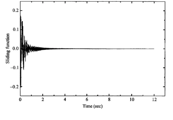
and

_(13).

Such defect can be also seen from

Figure

4,

which

_presents

the

_sliding

function for mt = 0.4.

During

the transient 0 < t <

2,

the _system

_trajectory

is not

_completely

constrained in the

_sliding

_{layer < E(= 0.01).}

It is because the

_system

tends to reach the control

_goal

as fast as

possible

from the

_starting

time.

As a

_result,

the control

_{input requires high-frequency}

_components to

_speed

_{up the}

_system

response

during

the transient.

Simultaneously,

the

high-frequency

unmodeled terms are also stimulated to

_degrade

the

_system

_response. After the

_transient,

the

_system

is well controlled

to the

_neighborhood

of the control

_goal.

That means the control

_input

intends to drive the

system

to the destination

_smoothly;

_therefore,

the

_{high-frequency}

unmodeled terms will not

Figure 2. _{Tip angle} for the cases of mt = 0.3, 0.4, 0.5 _kg.

Figure 4. _Sliding variable for mt = 0.4 kg.

5.

CONCLUSION

This _paper

_develops

a

sliding-mode

control of an FEM-based

single-link

flexible arm. Before

the controller

_design,

the FEM-based model is reduced via the Schur

_{decomposition}

to

_keep

only

the lower half of natural

_frequencies,

which are well estimated in the FEM-based model.

Simulation results are included to illustrate the robustness of the

_sliding-mode

control

_against

the

_payload

variation.

Acknowledgment. Research was _{supported by} National Science Council, _Taiwan, R.O. C., under Contract

NSC 86-2213-E-009-056.

REFERENCES

Bayo, E., 1987, "A finite-element approach to control the _end-point motion of a _single-link flexible robot," Journal _of Robotic Systems 4(1), 63-75.

Cannon, R. and Schmitz, E., 1984, "Initial _experiments on _end-point control of a flexible one-link robot," International Journal _{of Robotics 3(3),} 62-75.

Chang, J. L. and Chen, Y _P., 1997, "Force control of a single-link flexible arm _{using sliding-mode theory,"} Journal _of Vibration and Control 3(4), 439-452.

Golub, G. H. and Van _Loan, C. F., 1989, Matrix Computations, Johns Hopkins University Press, London.

Itkis, U., 1976, Control System of Variable _Structure, John _Wiley, New York.

Junkins, J. L. and Kim, Y, 1993, Introduction to _Dynamics and Control of Flexible Structure, AIAA, Washington, DC.

Matsuno, F., Murachi, T., and Sakawa, Y, 1994, "Feedback control of decoupled bending and torsional vibrations of flexible beams," Journal _{of Robotic Systems 11(5), 341-353.}

Nathan, P. J. and _Singh, S. N., 1991, "Sliding-mode control and elastic mode stabilization of a robotic arm with flexible

links," Journal of Dynamic System, Measurement, and Control 113, 669-676.

Utkin, V I., 1977, "Variable structure systems with sliding mode: A survey," IEEE Transactions on Automatic Control

22, 212-222.

Yeung, K. S. and Chen, Y P, 1989, "Regulation of a one-link flexible robot arm _{using sliding-mode technique,"} Inter-national Journal of Control 49, 1965-1978.