適用於ETC多車道環境下的執法演算法

國

立

交

通

大

學

資訊科學與工程研究所

碩

士

論

文

適用於 ETC 多車道環境下的執法演算法

A Non-payment Vehicle Searching Algorithm for ETC

Multi-Lane Free Flow Environment

研 究 生：林良叡

指導教授：簡榮宏 教授

適用於 ETC 多車道環境下的執法演算法

A Non-payment Vehicle Searching Algorithm for ETC

Multi-Lane Free Flow Environment

研 究 生：林良叡 Student：Liang-Rui Lin

指導教授：簡榮宏 Advisor：Rong-Hong Jan

國 立 交 通 大 學

資 訊 科 學 與 工 程 研 究 所

碩 士 論 文

Submitted to Institute of Network Engineering College of Computer Science

National Chiao Tung University in partial Fulfillment of the Requirements

for the Degree of Master

in

Computer Science

June 2011

Hsinchu, Taiwan, Republic of China

i

適用於 ETC 多車道環境下的執法演算法

研究生：林良叡 指導教授：簡榮宏 博士

國立交通大學資訊科學與工程研究所

摘

要

在電子收費（Electronic toll collection, ETC）系統中，利用車上機（On-Board Unit, OBU）與路邊節點(Roadside Unit, RSU)快速的資料交換，可降低收費處理 時間，進而提升車流量。ETC 系統由四個模組構成：自動車輛辨識模組、自動 車輛分類模組、扣款模組、影像執法模組。其中影像執法模組將每張車牌影像透 過自動化車牌辨識 (Automatic License Plate Recognition, ALPR) 產生牌照號碼， 再利用牌照號碼與車輛扣款資料比對找出未繳費與交易未成功之車輛。然而大量 的車牌辨識會造成 ETC 系統的瓶頸。此外牌照號碼與車輛扣款資料比對之運算， 多車道(Multi-Lane Free Flow, MLFF)比單車道(Single-Lane Free Flow, SLFF)來的 複雜。在本篇論文中，我們提出一個適用於 ETC 多車道環境下之模組，將車牌 影像資料和扣款資訊匹配關係轉換成雙分圖(Bipartite Graph)。針對雙分圖提出演 算法以找出未繳費與交易未成功之車輛。模擬的結果顯示出，我們提出的演算法 可大幅的降低影像辨識的次數並提高執法系統的成功率。

ii

A Non-payment Vehicle Searching

Algorithm for ETC Multi-Lane Free

Flow Environment

Student：Liang-Rui Lin Advisor：Dr. Rong-Hong Jan

I

NSTITUTE OF

C

OMPUTER

S

CIENCE AND

E

NGINEERING

N

ATIONAL

C

HIAO

T

UNG

U

NIVERSITY

Abstract

There are many benefits of electronic toll collection (ETC) system such as reducing toll paying time, increasing the capacity of toll station, decreasing fuel consumption, enhancing the convenience of traveler and so on. For a multi-lane free flow ETC system, how to find out the non-payment vehicles without recognizing all license plate images is an important research problem. In this thesis, we formulate the non-payment vehicle searching problem into a bipartite graph and propose an algorithm without recognizing all license plate images for solving it. Simulation results show that our algorithm can reduce the number of ALPR (Automatic License Plate Recognition) and increase success rate of enforcement.

iii

致謝

iv

Contents

Chapter 1 Introduction ... 1

1.1 VANETs and Electronic toll Collection ... 1

1.2 Motivations ... 5

Chapter 2 Related Works ... 7

Chapter 3 Bipartite-Graph-Based Algorithm ... 10

3.1 System Model ... 10

3.2 Bipartite Graph... 11

3.2.1 Graph property ... 13

3.2.2 Simplify Bipartite Graph... 14

3.3 Bipartite-Graph-Based Algorithm ... 16

Chapter 4 Simulation Result and Analysis... 22

4.1 Simulation Environment ... 22

4.2 Result Analysis... 24

4.2.1 Congested Traffic Analysis ... 24

4.2.2 Normal Traffic Analysis ... 26

4.2.3 Sparse Traffic Analysis ... 28

4.2.4 The degree Analysis ... 31

Chapter 5 Conclusion ... 32

v

List of Figures

Figure 1. (a) Multi Lane Free Flow (b) Single Lane Free Flow ... 3

Figure 2. Electronic toll collection Architecture ... 4

Figure 3 Virtual toll zone configuration in VPS system. ... 8

Figure 4 Using two report points to evaluate the lane position ... 9

Figure 5. An image data and the possible matching targets ... 11

Figure 6. A bipartite graph between image data and transaction data. ... 12

Figure 7. An example of the transaction data of v must be in N(v). ... 13

Figure 8. An example of the iamge data of u must be in N(u) ... 14

Figure 9. (a) Initial bipartite graph (b) The graph is processed by Property 5... 14

Figure 10. Two types of the charging vehicle ... 15

Figure 11. (a) Initial graph (b) After eliminate degree ... 16

Figure 12. The pseudo code of PT algorithm. ... 17

Figure 13. Flow Chart of Bipartite-Based Algorithm ... 19

Figure 14. (a)Plate5 is recognized as legal (b)Plate6 is recognized as illegal ... 20

Figure 15. (a) B01610 is legal (b) Remain two bipartite subgraph ... 21

Figure 16 Traffic flow at Taishan Toll Station a day. ... 23

Figure 17. Count of ALPR in congested traffic ... 25

Figure 18. Count of ALPR of each lane in congested traffic ... 25

Figure 19 Comparison of the number of degree in congested traffic ... 26

Figure 20 Counts of ALPR in normal traffic ... 27

Figure 21 Counts of ALPR of each lane in normal traffic ... 27

vi

Figure 23. Counts of ALPR in sparse traffic ... 29

Figure 24. Counts of ALPR of each lane in sparse traffic ... 30

Figure 25. Comparison of the number of degree in sparse traffic ... 30

vii

List of Tables

1

Chapter 1

Introduction

Owing to the dramatic cost down on electronic components and the advances on wireless technologies, the development of Intelligent Transportation System (ITS) has drawn intensive attention in recent years from many countries. The Vehicular Ad hoc Network (VANET) is a promising approach for the future ITS. In this novel architecture, vehicles can communicate with roadside units (RSU), referred to as vehicle-to-roadside (V2R) communication. In addition, vehicles can also communicate with each other in vehicle-to-vehicle (V2V) communications.

1.1 VANETs and Electronic toll Collection

The main characteristics of vehicular networks are high speed and frequent network topology changes. However, 802.11 doesn’t fit with above characteristics. The Intelligent Transportation Systems (ITS) Committee of the IEEE Vehicular Technology Society (VTS) define IEEE 802.11p/1609.X draft for VANET. The IEEE 1609 main provides the multi-channel operation. The Federal Communications Commission (FCC) of the U.S allocate 75MHZ Dedicated Short Range

2

Communication (DSRC) [1] spectrum within the (5.85-5.925) GHZ. The overall bandwidth is divided into seven channels which are composed of one control channel (CCH) and six service channels (SCHs). The CCH is mainly used to transmit safety-critical messages and high priority messages in the form of WAVE short message (WSM). The SCHs is mainly used to deliver non-safety messages.

There are two types of applications of VANET: 1) the safety applications and 2) the traffic information applications. The purpose of the safety application is to decrease the traffic accident. The mainly safety application are emergency messages and collision avoidance. The emergency messages are usually reserved at the specific zone for a long time so that the drivers can pay attention to the warning area. The Cooperative Collision Avoidance (CCA) [2] informs the backward vehicle the front road information so that the vehicle collision accident could be reduced. The common characteristic of the applications are that the messages should be propagated in low delay time reliably.

There are several kinds of traffic information applications such as the Global Position System (GPS) and Electronic toll collection (ETC).

In this thesis, we focus on the related issue of ETC. According to a research of traffic congestion on toll highways, the heaviest congestion occurs near toll gates, where vehicles make a short stop to pay the toll. Hence, the primary cause of traffic jams can be eliminated by creating an electronic-toll-collection system (ETC). Through wireless communication between the in-vehicle device (On-Board Unit, OBU) and the roadside antenna of a toll gate (RSU), vehicles are able to drive through toll gates without stopping. There are two types of ETC systems currently used in the world, called single-lane free flow (SLFF) as shown in Figure 1(a) and multilane free flow (MLFF) as shown in Figure 1(b), respectively. It is also known that multilane free-flow system is more convenient for faster traffic throughput due to the less

3

restriction on vehicle passing speed. MLFF also permit vehicle change the lane during collection so that the implement of the collection is more complicated than SLFF.

Figure 1. (a) Multi Lane Free Flow (b) Single Lane Free Flow

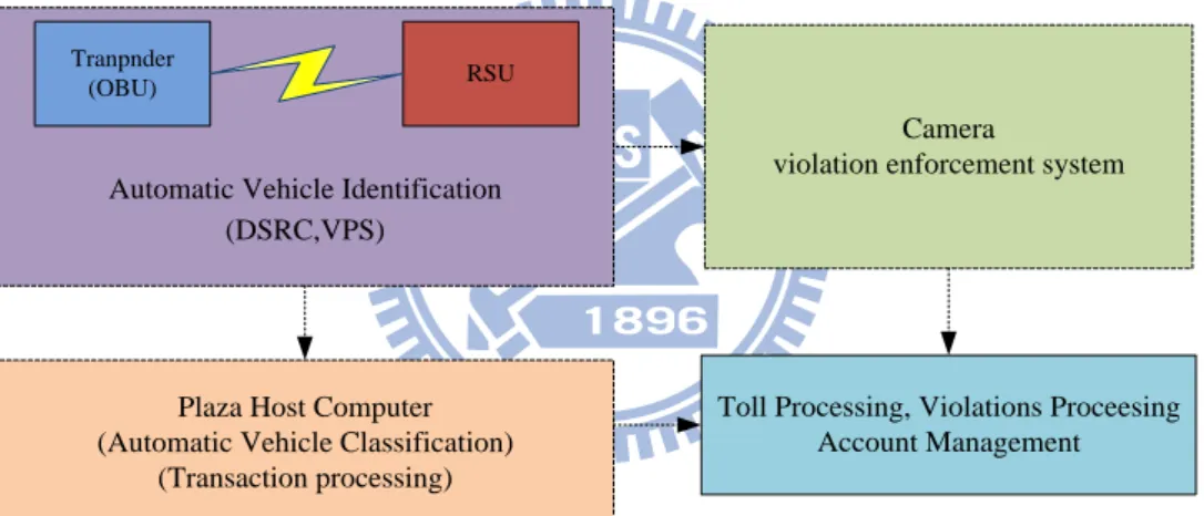
As shown in Figure 2, a typical ETC system has four modules [4]: 1) Automatic Vehicle Identification (AVI); 2) Automatic Vehicle Classification (AVC); 3) transaction processing; and 4) violation enforcement system (VES). The AVI component involves the use of OBU-to-RSU communications to identify the vehicle when entering the toll gate area. The type of OBU can be either a transponder or a radio-frequency identification (RFID) tag so that the vehicle can automatically be identified. The communication technology of ETC can be classified into two types of categories: DSRC-based system and Vehicle Position System (VPS). DSRC-based system has two main communication technologies: Infrared and microwave. The infrared communication technology is mature and low cost, and has the feature of fewer channel collision. The advantages are easy installation and maintenance. It is easily

(b) (a)

4

affected by weather conditions and is suitable for only SLFF. Microwave communication system is mostly adopted in many countries now. There are several carrier frequency being utilized, such as 915MHz, 2.4-GHz, and 5.8-GHz. Microwave is suitable for the MLFF, thus it can increase traffic flow throughput. Compared to Infrared, the microwave propagation will be affected by the environment and interference with each other. To install the microwave RSU, it must be tested and analyzed the interference caused by different topology. VPS combines GPS and mobile communication. The vehicle could report its real-time position to the server and the driver could receive the bills by cell phone. Because of the high precision requirement of the vehicle position, the technique is still not matured.

Toll Processing, Violations Proceesing Account Management Automatic Vehicle Identification

(DSRC,VPS)

Tranpnder

(OBU) RSU

Plaza Host Computer (Automatic Vehicle Classification)

(Transaction processing)

Camera

violation enforcement system

Figure 2. Electronic toll collection Architecture

For AVC component, vehicle class can be determined by the vehicle’s physical characteristics, such as the number of axles. A higher toll is usually imposed on vehicles with more axles. Larger commercial trucks or vehicles pulling trailers, therefore, would likely pay a higher toll.

Transaction processing entails debiting the toll from the customer’s account and addressing customer inquiries. Violation enforcement usually includes cameras to

5

capture an image of license plates, and a license plate reader system to recode photographs and license plate numbers of all vehicles. Thus, automatic license plate recognition (ALPR) technology is often used in violation enforcement.

1.2 Motivations

The most common current practice in violation enforcement involves determining and sending out written notices for each violation. Since the accuracy of ALPR is not always reliable, human review and correction will be needed to improve the accuracy of the license plate reading. However, recognizing a large number of photographs will cause a large number of human reviews and corrections will increase the cost of ETC system. In SLFF, it is easy to match the vehicle’s transaction record to its image record correctly because both of these record must take place at the same lane; however, in MLFF, it is relatively complicated to match the vehicle’s transaction record to its image record correctly because of the vehicle may change the lane and it may occur that transaction record can’t match with image record.

In this thesis, we focus on improving the efficiency of VES. In order to solve the problem of matching the correct transaction data to correct license plate image data, we propose a bipartite graph matching solution which not only can reduce the human loading but also can accurately identify the vehicles that drive through a highway toll gate area without paying for toll. To match the vehicle’s transaction data to its license plate image data correctly, ALPR technology is one of the important factors. As mentioned above, the precision of the ALPR is not reliable. To reduce the count of the ALPR, we propose the bipartite-graph-based algorithm to cope with the bipartite graph. Simulation result shows that our method doesn’t need to recognize each picture, so that it can increase the accuracy to verify the illegal vehicle which doesn’t pay the toll.

6

The rest of this thesis is organized as follows. In chapter 2, we reviewed the related works. Then, we introduce that how to construct the bipartite graph and utilize the divide-and-conquer algorithm to decrease the count of ALPR. Chapter 4 shows our simulation results and analysis. Finally, this thesis is concluded in Chapter 5.

7

Chapter 2

Related Works

ETC needs serious accuracy and feasible. Several studies have been proposed to design the architecture for ETC [4]. Some researches were proposed for AVI components.

In [5], the authors designed in-pavement antennas with carrier frequency 915MHZ. The tag is on the lower edge of the front license plate, and the in-pavement antennas are buried under the road. The transmission range is one meter wide and 2 meter high. It support variable bits packet for several operations. However, it is not sufficient for congested traffic. In [6] the authors proposed MLFF architecture for ETC. The gantry is 6.2m height cross the width of three lanes and the transceivers are with carrier frequency 5.8GHz. In [7] the authors proposed a novel architecture by employing millimeter-wave range in MLFF. Each lane is equipped with antennas and the frequency of each is different. The proposed scheme utilized high resolution in lateral directions to track the vehicle’s direction. This is for separating the packets into segments so that can communicate with RSU consecutively. The communication range may overlap on the intersection of adjacent lane.

Some researches were proposed for AVC components. In [8], the authors proposed a wire device that can get the electronic signal when vehicle passing. The device can classify type of vehicles by the variation signal information. ETC System can utilize the information to toll different amount of money.

8

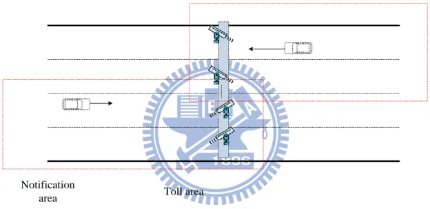
Some researches were proposed for Enforcement System. In [9] proposed VPS scheme. As shown in Figure 3, the toll zone is a rectangle area on each direction and covers the range the vehicles may pass. The coordinate of virtual toll is stored on OBU, so vehicles can know whether they drive in the area by GPS. The area has two parts: Notification area and toll area. When vehicles pass through the notification area, OBU is ready for paying tolls. The vehicle would send transaction request message to back server in RSU. The vehicle’s plate number is sent to RSU for matching the license image. However, ALPR is not reliable and it has to recognize every image.

Notification

area Toll area

Figure 3 Virtual toll zone configuration in VPS system.

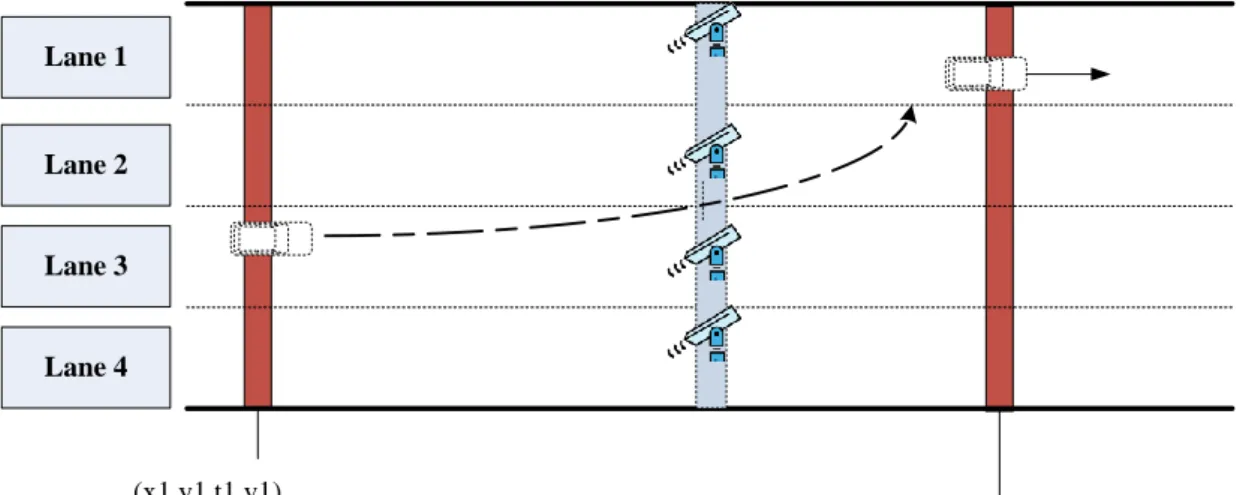
In [10], the authors proposed the enforcement system, the system using the transaction to find the mapping image data. If not found, the system would keep find according the order of lane. If still not found, entering the human checking review. In [11], the authors proposed the method to increase the success rate to matching the image data and transaction data. As shown in Figure 4, there are two report points. At these points, the vehicle would report his current coordinate to RSU. The two coordinates can compute the position where the vehicles are taken pictures. Servers can just only check the image data that located at the possible lane. However, the

9

method is still to recognize all the image data so that to map the transaction data. The follow chapter would introduce our algorithm that is efficient and doesn’t need recognize all the image data.

(x1,y1,t1,v1) (x2,y2,t1,v2) Lane 1 Lane 2 Lane 3 Lane 4

10

Chapter 3

Bipartite-Graph-Based Algorithm

In this chapter, we introduce our bipartite-graph-based algorithm. In section 3.1, the system model is described. In section 3.2, we transfer our problem into bipartite graph and introduce the characteristic of the graph. In section 3.3, utilizing divide-and-conquer algorithm to cope with bipartite graph decreasing the count of ALPR. In section 3.4, is the whole view of our algorithm.

3.1 System Model

In the system model, we suppose the scenario of the road is a highway with 4-lanes considering single direction. In this thesis, we assume of the vehicles on the road equip with positioning devices such as GPSs to acquire their own position. There is a RSU to provide the AVI service and several cameras on each lane in the toll collection plaza. We supposed that the communication between RSU and OBU is 802.11p/1609. Utilizing WAVE/DSRC has more extensive transmission range than DSRC-based ETC system.

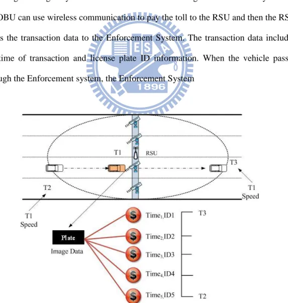
Different from the traditional architecture, the vehicles can communicate within the RSU’s transmission range in our model as shown in Figure 5 ( the area of the

11

dotted ellipse ), it means that the positions of tolls which occur in the range and are not restricted before the RSU.

3.2 Bipartite Graph

A bipartite graph is an undirected graph G = (V, E) which vertices can be partitioned into two disjoint sets V1 and V2 such that (u, v) ∈ E, u ∈ V1 and v ∈ V2. The primary step is to create a bipartite graph representation of the relation between license plate image data and transaction data. The flow for creating a bipartite graph is described as follow: As shown in Figure 5, consider a vehicle equipped with an OBU is driving on a highway. When the vehicle enters the toll gate area defined by a RSU, the OBU can use wireless communication to pay the toll to the RSU and then the RSU sends the transaction data to the Enforcement System. The transaction data includes the time of transaction and license plate ID information. When the vehicle passes through the Enforcement system, the Enforcement System

12

will take a picture of the license plate in order to get the license plate image data. At the same time, the Enforcement System gets the speed (V2) of the vehicle and uses the

time of taking the picture (T1) to infer the time of entering the toll gate area (T2) and

exiting the toll gate area (T3). The time of T2 and T3 can be computed by

𝑣22 = 𝑣12+ 2𝑎𝑠

𝑣₂ = 𝑣₁+ 𝑎𝑡 𝑡 =2𝑠_𝑣

2

Let the speed of vehicle which enter the communication (V1) is equal to zero, and the

transmission area of the RSU is S, then we can infer the threshold time of passing the transmission area to ensure that all the image data could map to whole possible transaction data. All the transaction data from T3 to T2, said the possible matching

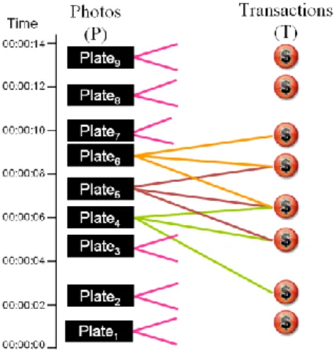
targets, will be connected to the image data. As the shown example in Figure 5, there are five transaction data from T3 to T2. So the image data has five possible matching

targets. As shown in Figure 6, for each image data, we can connect it with the corresponding transaction data and then a maximum connected bipartite graph G (PT, E) is created, where the set of vertices P represents image data, the set of vertices T represents transaction data and the set of edges E represents links between P and T.

13

3.2.1 Graph property

Let G(V, E) be a graph and vV(G) be a vertex. Given P ={𝑃1, 𝑃2, ……, 𝑃𝑚} set

of image data, T={𝑡1, 𝑡2, ……, 𝑡𝑛} set of transaction data and 𝐸={(𝑃𝑖, 𝑇𝑗)│there

exists some possible transactions are the matching targets of license plates according velocity acquired during taking pictures.}

We use the notation N(v) and E(v) to denote the set of vertices connected to v and the set of edges incident with v, respectively. The cardinality |E(v)| is called the degree of v, denoted by deg(v). Consider a maximum connected bipartite graph G(PT, E)

representing the relation between license plate image data and transaction data. Then

G(PT, E) has the following properties:

Property 1. The number of vertices of the image data set P is greater or equal to the number of vertices of the transaction data set T.

1.1 If |P| = |T|, all the vertices in P are legal vehicles. It means that all these vehicles drive through the toll gate area with paying for toll. 1.2 If |P| > |T|, there exists at least one illegal vehicle in P without

paying for toll.

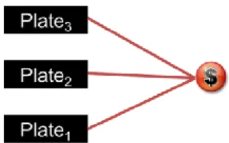
Property 2. For a vertex v in P, if v is a legal vehicle, the transaction data of v must be in N(v). It means that the transaction data of v is in the set of possible matching targets of v. As shown in Figure 7.

Figure 7. An example of the transaction data of v must be in N(v).

14

Property 4. For a vertex u in T, the image data of u must be in N(u). As shown in Figure 8.

Figure 8. An example of the iamge data of u must be in N(u)

Property 5. For a vertex u in T, if deg(u) = 1 and vertex v is the only neighbor of u, v is a legal vehicle and u is the transaction data of v.

Figure 9. (a) Initial bipartite graph (b) The graph is processed by Property 5.

Consider an example of a bipartite graph as shown in Figure 9(a), the transaction data with the license plate ID is P01802, B00010, and A21787, each of them has the only one in-degree, so we can say that plate1 is mapping to P01820, plate2 is mapping to B00010, and plate3 is mapping to A21787, then, we can remove irrelevant edges which are connected to the transaction data. Figure 9(b) shows the result after processing by Property 5.

3.2.2

Simplify Bipartite Graph

In the congested environment, the speed of vehicles is relative slow. It means that there are numerous vehicles stay in the transaction area at the same time. Thus,

15

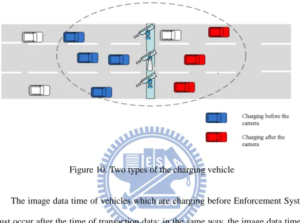
each of the image data could map to as much as possible transaction data. We assume all of the vehicles that equip OBUs would report their own position to server during paying tolls. As shown in Figure 10, there are two types of the charging vehicles in the transaction area. One is charging before the camera, and the other is after the camera.

Figure 10. Two types of the charging vehicle

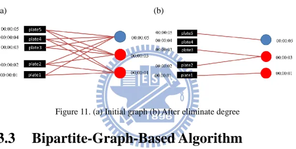
The image data time of vehicles which are charging before Enforcement System must occur after the time of transaction data; in the same way, the image data time of vehicles which are charging after Enforcement System must occur before the time of transaction data. Using the above characteristic could eliminate unnecessary image data’s out-degree to transaction data. Consider an example as shown in Figure 11, The red circles are the vehicles which paid tolls after Enforcement System and the blue circle is the vehicle which paid tolls before the Enforcement System. The time of the blue circle is 00:00:05, so the time of possible image data must after 00:00:05, so the blue circle has only one in-degree that connected to the plate5. The time of the red circles are 00:00:03 and 00:00:01 each, so the time of possible image data are plate1, plate2 and plate3.

16

ID where the vehicles are taken images on, then we classify the image data and transaction data according to the lane ID, for example the number of lanes are four, we can divide the original bipartite graph into four subgraph, this would decrease the number of degree of each vertex in G. Reducing the number of degrees would improve our algorithm performance, the impact of the factor will investigate in Chapter 4 and compare to the original bipartite graph, partition graph by charging position and partition by lane ID.

(a) (b)

Figure 11. (a) Initial graph (b) After eliminate degree

3.3 Bipartite-Graph-Based Algorithm

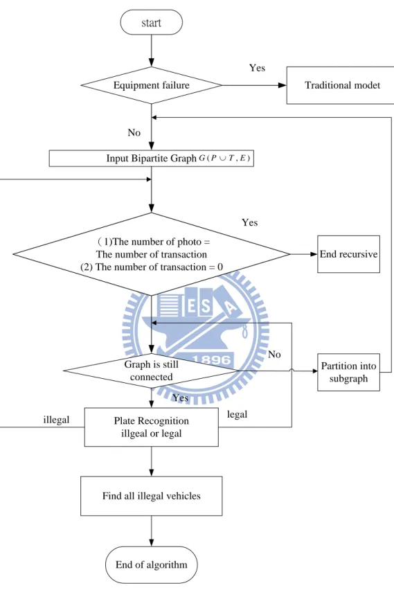
We design an algorithm to discover the illegal vehicles which are not equipped OBUs efficiently by utilizing the graph property above mentioned. As shown in Figure 12, the main spirit of the algorithm here is the use of Property 1. When the number of vertices of the image data set is equal to the number of vertices of the transaction data set, it can determine all the image data are legal vehicles quickly and reduce the number of image recognitions. On the other hand, if the number of image data is greater to the number of the transaction data, there exists at least one illegal vehicle in image data set. In this case, the image recognition processing can make that the two sets have the same number of vertices or disconnect the bipartite graph into disjoint components. For each component, it is recursive and used as the input of the

17 algorithm.

Figure 12. The pseudo code of PT algorithm.

The details are described as follows :

 line 1 and 2: Explain the input and output.

 line 3: The input is a maximum connected bipartite graph G(PT, E)

 line 4 ~ line 6: Apply Property 1.1 to check whether the number of vertices of 1 Input: a maximum connected bipartite graph G(PT, E).

2 Output: two sets of illegal vehicles and legal vehicles. 3 Input (G(PT, E)) {

4 If |P| = |T|

5 move u into the set of legal vehicles, uP; 6 exit;

7 If |P| = 1 and |T| = 0

8 move u into the set of illegal vehicles, where uP; 9 exit;

10 run Check_Degree_One_Vertices_In_T;

11 If G is disconnected and has G1, G2, …, Gn components

12 Gi, Input(Gi(PiTi, Ei)), i = 1, 2, …, n;

13 else {

14 while (G is connected and G is not empty) { 15 take the middle node uP;

16 Image_Recognition(u); 17 If (License_check(u) = true)

18 move u into the set of legal vehicles; 19 else {

20 move u into the set of illegal vehicles; 21 If |P| = |T|

22 move u into the set of legal vehicles, uP; 23 exit;

24 }

25 run Check_Degree_One_Vertices_In_T; 26 }

27 If G is disconnected and has G1, G2, …, Gn components

28 Gi, Input(Gi(PiTi, Ei)), i = 1, 2, …, n;

29 } 30 }

18

image data set is equal to the number of vertices of transaction data set or not. If agree, all image data are legal and moved to the set of legal vehicles.

 line 7 ~ line 9: Apply Property 3 to check whether the number of vertices of image data set is equal to one and the number of vertices of transaction data set is equal to zero. If agree, the only image data is illegal and moved to the set of illegal vehicles.

 line 10: Run the Check_Degree_One_Vertices_In_T function. By Property 5, for a vertex in transaction data set with degree one, the only neighbor of this vertex must be legal and can be moved to the set of legal vehicles.

 line 11 ~ line 12: If G is disconnected and has some components after the steps above, the components can be recursive and used as the input of the algorithm.

 line 13 ~ line 29: Use the image recognition processing repeatedly until the two sets of image data and transaction data have the same number of vertices or G is disconnected.

19

（1)The number of photo = The number of transaction (2) The number of transaction = 0

Graph is still connected Yes Plate Recognition illgeal or legal End recursive Yes Partition into subgraph No illegal legal start Equipment failure

Find all illegal vehicles

End of algorithm

Input Bipartite Graph G(PT,E)

Yes

Traditional modet

No

20

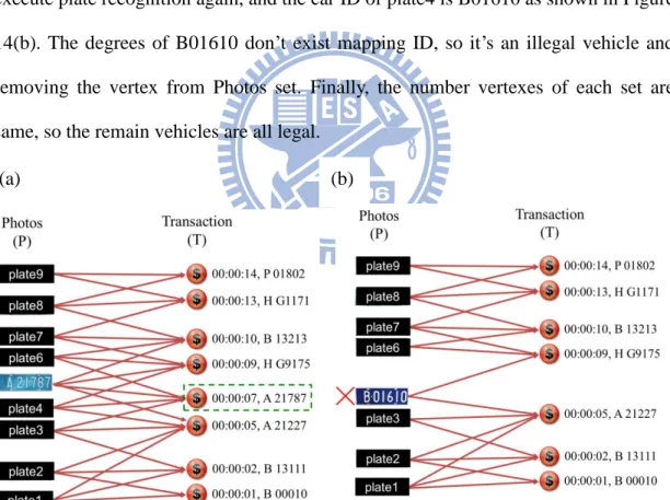
We take two examples to explain the whole Bipartite-Base Algorithm. Consider the set of image data have nine vertexes, and the set of transaction have eight vertexes, so it means that there is an illegal vehicle. To find the illegal vehicle, taking the middle vertex plate5 of the Photos set to execute plate recognition first, the car ID of plate5 is A21787 as shown in Figure 14(a). The degrees of A21787 exist mapping ID, so it’s illegal. Second step is removing the vertex from Photos set, and eliminating the degrees which are connected to transaction data A 21787. The bipartite graph is still connective and the number vertexes of Photo set are still more than the number vertexes of Transaction set, so taking the middle vertex plate4 of the Photos set to execute plate recognition again, and the car ID of plate4 is B01610 as shown in Figure 14(b). The degrees of B01610 don’t exist mapping ID, so it’s an illegal vehicle and removing the vertex from Photos set. Finally, the number vertexes of each set are same, so the remain vehicles are all legal.

Figure 14. (a)Plate5 is recognized as legal (b)Plate6 is recognized as illegal

Consider another example as shown in Figure 15. We assume that B01610 is legal now, then the vertex B01610 of Photos set is removed, and all the edges which are connected to the vertex B01610 of Transaction set are removed too. The bipartite

21

graph is disconnected as shown in Figure 15 (b). There are two subgraph, one of has four vertexes of each set, so remain four vehicles are all legal. On the other hand, another subgraph has three vertexes in Photos set and two vertexes in Transaction set, it means that there is one illegal vehicle in the subgraph. The components can be recursive and used as the input of the algorithm to find remain illegal vehicle.

Figure 15. (a) B01610 is legal (b) Remain two bipartite subgraph

22

Chapter 4

Simulation Result and Analysis

4.1 Simulation Environment

In this chapter, we show the simulation result of our algorithm and its performance.In [12], the mobility generator has including Random Waypoint model, Reference Point Group Mobility model, Reference Point Group Mobility model and Man-attan mobility model. It is used in our simulations to generate mobility scenario for the Freeway Model. As mentioned in Chapter 3, the simulation scenario is in an 4km highway with 4 lanes considering single direction. We conduct the simulation using ns-2 simulator [14]. We evaluate our alogrithm on three scenarios for congested, normal, and sparse traffic. As mentioned in 3.2.2, we compare the ALPR count of orginal bipartite graph and simplified graph.

The tolerant of the traffic flow in Taiwan ETC is 2,210 vehicles/hour in the rush hour [13], as shown in Figure 16, the most vehicles appear at 10am to 21pm, and the total traffic flow is almost 8000 vehicles an hour for all lanes. Electronic toll collection have been implemented in Taiwan for five years, the proportion of illegal vehicles which are not equipped OBUs to total traffic flow as show in Figure 16. The average error rate is closed to 0.06% recent years. In our simulation, we utilized the error rate from 0.06% to 3.0% in the three scenarios.

23

Figure 16 Traffic flow at Taishan Toll Station a day.

http://211.79.135.72/volume/drawday.htm

Figure 16 Traffic flow at Taishan Toll Station a day.The proportion of illegal vehicles

We have three different scenarios: congested traffic, normal traffic, and sparse traffic. The main different parameters between these scenarios are the velocity, number of vehicles and acceleration. Table 1 showed our simulation parameters details.

24

The Length of Highway 4000m

Number of lanes 4 lanes

Number of Vehicles [4410, 3286, 2519] Velocity Vmax:[108, 80, 54]Km/h Vmin:[90, 72, 36] Km/h Acceleration Speed [0.4, 0.8, 1.2]m/s2 Simulation times 1800s Transmission Range 100m

Location of the camera 2000m

Location of the RSU 2000m

Table 1. Simulation Parameters

4.2 Result Analysis

In this section, we compare the count of ALPR in three different traffic scenarios: congested traffic, normal traffic, and sparse traffic.

4.2.1 Congested Traffic Analysis

Figure 17 shows the count of ALPR in congested traffic, as the ratio of count of ALPR increasing faster the error rate growing larger. In the worst case, the count of ALPR is almost closed to the number of total vehicles. The reason is that our algorithm has to check vertexes continuously until the number vertexes of each set are equal or bipartite graph becomes disconnected. In other words, it has to recognized amounts of picture to achieve the terminate condition of algorithm. The simplified method as mentioned in chapter 3.2.2, we named the method by relative position to camera as “PPC” which is abbreviation of partition by position of camera and the method by partition by lane as “PL” which is abbreviation of partition by lane. PPC still need the count more than half of the total vehicles, because the partite graph still has many vertexes exist in each set. Combining with PPC and PL achieve better

25

performance than original graph and PPC graph. By utilizing PPC, the count of ALPR is reduced to 15%. By exploiting PL with PPC, the count of ALPR is reduced to 60%. Figure 18 presents counts of ALPR of each lane by utilizing PL and PPC. Obviously, the count gets larger as the error rate grows up.

Figure 17. Count of ALPR in congested traffic

Figure 18. Count of ALPR of each lane in congested traffic 0 50 100 150 200 250 300 350 0.10% 0.60% 1.20% 2.00% 3.00% co u n t of A LP R error rate lane1 lane2 lane3 lane4

26

Figure 19 Comparison of the number of degree in congested traffic

Figure 19 shows that the comparison of the number of degree, the number of original bipartite graph is eight times degree as much as PL plus PPC during 300s to 500s. This claims that if we want to get the good performance of Bipartite-Based Algorithm, the number of degree is an impact factor.

4.2.2 Normal Traffic Analysis

Figure 20 shows that the ratio of count of ALPR increasing faster the error rate growing larger. The count is still half of the total vehicles by utilizing original graph in worst case. The reason is same as in congested traffic. Compared with the congested traffic, the ratio of counts is reduced. By utilizing PPC, the count of ALPR is reduced to 23% compared to origin. By exploiting PL with PPC, the count of ALPR is reduced to 80% compared to origin. The ratio of counts of ALPR in normal traffic decreased much more than in congested traffic. As shown in Figure 21, presents counts of each lane of ALPR by utilizing PL and PPC. Obviously, the counts in the

27

worst case of normal traffic are one-third to congested traffic.

Figure 20 Counts of ALPR in normal traffic

Figure 21 Counts of ALPR of each lane in normal traffic 0 20 40 60 80 100 120 0.10% 0.60% 1.20% 2.00% 3.00% co u n t o f A LP R error rate lane1 lane2 lane3 lane4

28

Figure 22. Comparison of the number of degree in normal traffic

Figure 22 shows that the distribution of counts of degree. In normal traffic, the count of degree is half of the congested traffic. The count of vehicles is also fewer during the same time period.

4.2.3 Sparse Traffic Analysis

Figure 23 shows that the ratio of count of ALPR increasing faster the error rate growing larger. By exploiting PL with PPC reduced 87% of count of ALPR compared to origin. By utilizing only PPC reduced 36% of count of ALPR compared to origin. The count of ALPR in sparse traffic is the smallest one compared to other scenarios. Clearly, even in the worst case, PL with PPC cost only 5% counts of total vehicles. The velocity is faster and relative density is lower, this would cause the bipartite graph existed some disconnected components at beginning by exploiting PL with PPC.

29

Figure 24 present the count of degree each lane under PL with PPC. Compared to another two scenarios, the count of degree is much lower. Figure 25 shows the average per ten seconds, the count of degree of PL with PPC is fewer than five. In sparse traffic, the bipartite graph has many components and some of them have exactly the same number of vertexes of transaction set and pictures set by using PL with PPC so that the partite graph doesn’t need to check as many as vertexes to let the graph be disconnected.

30

Figure 24. Counts of ALPR of each lane in sparse traffic

Figure 25. Comparison of the number of degree in sparse traffic 0 5 10 15 20 25 30 35 40 45 50 0.10% 0.60% 1.20% 2.00% 3.00% co u n t o f A LP R error rate lane1 lane2 lane3 lane4

31

4.2.4 The degree Analysis

Figure 26 shows the number of degree in three scenarios with original graph and simplified graph. The count of degree is the most by exploiting original graph. It seen to has closed count of degree by utilizing PL with PPC in each scenario, but our simulation show the count of degree in dense is ten times more than in sparse. This is because the number of vehicles in dense is much more than in sparse during the same time period. In other words, it has to check as many as vertexes so that the bipartite graph could be disconnected.

Figure 26. The average count of degree in each scenario.

32

Chapter 5

Conclusion

In this thesis, we proposed a bipartite-graph-based algorithm for Enforcement System. The accuracy of ALPR is not always reliable, human review and correction will be needed to improve the accuracy of the license plate reading. Our algorithm could discover the illegal vehicles automatically, and it could decrease the count of human review and ALPR. It is suitable for MLFF environment and reliable. The simulation results shows that if the bipartite graph is without processing, the original bipartite graph had bad performance under the congested scenario. We proposed two methods to simplify the graph, one is according the position of transaction data relative to the cameras, and another is according the lane position where the vehicles were taken by cameras. Simulation results show good performance by simplifying the bipartite graph. In conclusion, our algorithm is more feasible and reliable for ETC enforcement.

33

Reference

[1] L. Armstrong, “Dedicated Short Range Communications (DSRC),” [Online]. Available: http://www.leearmstrong.com/dsrc/DSRCHome.htm

[2] S. Biswas, R. Tatchikou, and F. Dion, “Vehicle-to-vehicle wireless communication protocols for enhancing highway traffic safety,” IEEE Communications Magazine, vol. 44, no. 1, pp. 74-82, 2006.

[3] K. V. N. Kavitha, A. Bagubali, and L. Shalini, “V2V wireless communication protocol for rear-end collision avoidance on highways with stringent propagation delay,” In Proceedings of the International Conference on Advances in Recent Technologies in Communication and Computing (ARTCom 2009), pp. 661-663, 2009.

[4] Z.H. Xiao, Z.G. Guan, Z.H. Zheng, “The Research and Development of the Highway's Electronic Toll Collection System,” International Workshop on

Knowledge Discovery and Data Mining, pp. 359-362, 2008

[5] C. M. Walker and W. K. Brockelsby, “Automatic Vehicle Identification (AVI) technology design considerations for highway applications,” in Proc. 41st IEEE

Vehicular Technology Conf., Gateway to the Future Technology in Motion, 1991,

pp. 805–811.

[6] M. A. S. Mustafa, M. Pitsiava-Latinopoulou, and G. A. Giannopoulos,“The multilane electronic toll collection system in Thessaloniki: Evaluation of its first 6 months of operation,” in Proc. IEEE Vehicle Navigation and Information

Systems Conf., 1994,pp. 699–703.

34

multilane-free-flow electronic-toll-collection systems in the millimeter-wave range,” IEEE Trans. Intell. Transp. Syst., pp. 294–301, 2005

[8] Bertrand, Jean and Dicko, Mamadou,“Method and device for classifying vehicles＂U.S. Patent NO. 20030163263

[9] Lee, W.H., Tseng, S.-S., Wang, C.-H.: “Design and Implementation of Electronic Toll Collection System Based on Vehicle Positioning System Techniques.”

Computer Communications, 31(12), pp. 2925–2933, 2008

[10] 中華電信股份有限公司,“多車道自由流電子收費系統逃/欠費偵測機制＂中 華民國發明專利第533382號

[11] 中華電信股份有限公司, “一種提升VPS電子收費系統之扣款資料與執法資 料自動匹配作業成功率的方法,＂中華民國發明專利第200839652號

[12] “F. Bai, N. Sadagopan, and A. Helmy. User Manual for IMPORTANT Mobility

Tool Generators in ns-2 Simulator. University of Southern California, February

2004.

[13] “Taiwan Area National Freeway Bureau”. [Online]. Available: http://www.freeway.gov.tw

[14] “The network simulator: NS-2,” [Online]. Available: http://www.isi.edu/nsnam/ns/