經營環境調整後之中國大陸全域型銀行效率分析

全文

(1)國立交通大學經營管理研究所碩士論文. 經營環境調整後之中國大陸全域型銀行效率分析 Operational Environment-adjusted Bank Efficiency in China. 研究生：李志元指導教授：胡均立教授. 中華民國九十六年一月.

(2) 經營環境調整後之中國大陸全域型銀行效率分析 Operational Environment-adjusted Bank Efficiency in China. 研究生：李志元. Student：Chih-Yuan Lee. 指導教授：胡均立. Advisor：Dr. Jin-Li Hu. 國立交通大學經營管理研究所碩士論文. A Thesis Submitted to Institute of Business and Management College of Management National Chiao Tung University in Partial Fulfilment of the Requirements for the Degree of Master of Business Administration. January 2007 Taipei, Taiwan, Republic of China 中華民國九十六年一月.

(3) 經營環境調整後之中國大陸全域型銀行效率分析研究生：李志元. 指導教授：胡均立. 教授. 國立交通大學經營管理所碩士班中文摘要. 本研究使用四階段資料包絡分析法分析 1995 年到 2004 年十一家中國大陸全域型銀行的經營效率。除了人為管理因素影響之外，各銀行所處的環境亦會形成對銀行經營有利與不利的因子，而本研究之目的即在於將純粹管理上的無效率，和經營環境所造成的無效率，從整體無效率中分解出來。本研究之模型係採用投資、放款兩個產出變數，以及存款、員工數和固定資產等三個投入變數。所有的名目數據資料皆經過以 1995 年為基期的 GDP 物價平減轉換為實質變數以進行研究分析。透過 Tobit 複回歸模型來估計銀行的成立年數、所有權型式、政策影響、存放比率、銀行規模、世界貿易組織的參與以及亞洲金融風暴等人為管理之外的外生變數，是否會對理論投入值與實際投入值所產生的差額數值產生顯著性的影響。在經過去除環境因子影響的調整後，大陸的國有銀行之效率值均獲得大幅度提升，意謂著現階段的經營環境的確比較有利於股份制銀行的經營，如果無法適應經營環境，國有銀行可以藉由所有權的改革以提升經營效率。. 關鍵詞: 資料包絡分析法，銀行績效，環境調整，差額變數測量，無效率分解，中國金融. i.

(4) Operational Environment-adjusted Bank Efficiency in China Student: Chih-Yuan Lee. Advisor: Dr. Jin-Li Hu. Institute of Business and Management National Chiao Tung University ABSTRACT Applying the four-stage data envelopment analysis (DEA) approach proposed by Fried et al. (1999), this thesis studies the operational environment-adjusted efficiency of eleven nationwide banks in China from 1995 to 2004.. In addition to managerial factors,. the operational environment also brings favorable and unfavorable effects to banks. This study attempts to separate the inefficiency caused by management and inefficiency caused by operational environment.. There are two outputs (investment and loans) and three. inputs (deposits, employees, and fixed assets) in the DEA model. All nominal variables are transformed into real variables by the GDP deflators at the 1995 price level.. After. adjusting the input variables by excluding effects caused by environmental factors, state-owned banks have a greater improvement on efficiency.. This implies that the. joint-equity ownership significantly favors nationwide banks in China.. State-owned banks. can hence engage in ownership reform to improve their efficiency. Keywords: data envelopment analysis, DEA, banking efficiency, environment-adjusted, slack-based measure, decomposition of inefficiency, banking, China. ii.

(5) ACKNOWLEDGEMENT 初春，微冷，渺渺小雨，今天改搭乘捷運到學校來，早上十點以後台北城西的街道上，我的步調其實並不算得上慵懶，但跟著其他人比較起來，我倒是不那麼的急促，今天的進度是把這篇致謝辭寫完，然後整個兩年來的學習研究之路就算是完成。然而，在可以寫致謝辭之前，每一篇論文都是經過一陣為期不短煎熬、陣痛，才得以大功告成。我坐在老師研究室的沙發上，伴著熱氣裊裊上騰的咖啡，然後把過程中幫助過、支持過我的每一位，打從心裡好好的感謝。父母長期以來的栽培與無形支持上的鼓勵，讓我可以毫無顧慮的完成學業；指導教授胡均立老師在課業修習與論文寫作的指導上亦耗費了不少心力；特別是內人姿儀，在人生路途上的溫馨陪伴與周全的打點，在失意落寞時的支持，在小成喜悅時的分享，都讓我感動至極；即將出世的寶寶，在爸爸努力論文寫作的夜晚，還不時在媽媽肚子裡快樂地擺動，就似敲鑼打鼓般地給我加油和打氣。當然，曾芳代教授與周雨田教授在論文初稿審查時具體的審查建議，與周雨田教授、蔡智發教授以及許牧彥教授在口試時的指點和意見，從學理與觀念上的糾正和指教，亦使本論文得以順利付梓。還要感謝研究室裡平時嘰嘰喳喳的同學們，尤其是柏毅和雅媚在論文議題上的相互切磋，理平、穎政、瑋含等酒肉損友在 saki 和 ale 上的陪伴，以及交大經管所壘球隊的球友，讓研究所的求學生活增添一點青春的活力與喜氣。. 李志元謹誌 2007 年 1 月. iii.

(6) Content Chinese abstract.........................................................................................................................i English abstract ........................................................................................................................ii Acknowledgement....................................................................................................................iii Content. .................................................................................................................................iv. List of Tables .............................................................................................................................v List of Figures ..........................................................................................................................vi 1. Introduction ..........................................................................................................................1 1.1 Background of banking in China ..............................................................................1 1.2 Research motivation ...................................................................................................2 1.3 Research objective ......................................................................................................5 2 Literature Review ..................................................................................................................7 2.1 Literature review of Data Envelopment Analysis approach...................................7 2.2 Literature review of bank efficiency around the world ..........................................7 2.3 Literature review of bank efficiency in China .......................................................13 2.4 Literature review of efficiency focused on environment-adjusted analysis ........16 2.5 A brief summary of the literature reviews..............................................................20 3. Methodology........................................................................................................................21 3.1 Theory of banking evaluation and variable definition..........................................21 3.2 CRS models of Data Envelopment Analysis...........................................................22 3.3 Four-stage DEA approach .......................................................................................25 3.4 Tobit regression model .............................................................................................31 3.5 Data ............................................................................................................................31 4. Empirical Results................................................................................................................38 4.1 Stage one: Initial DEA..............................................................................................38 4.2 Stage two: Quantifying the effect of the operational environment ......................40 4.3 Stage three: Data adjustment ..................................................................................42 4.4 Stage four: Re-compute CRS efficiency measures.................................................44 5. Concluding Remarks..........................................................................................................48 References................................................................................................................................50 References in Chinese.....................................................................................................50 References in English .....................................................................................................51. iv.

(7) List of Tables Table 1.. Business changes of the state-owned and stock-shared banks in China from 1996 to 2003.............................................................................................................3. Table 2.. The growth of investments, loans and deposits of banks from 1996 to 2003 .....4. Table 3.. Classification and names of sample banks..........................................................32. Table 4.. Description of input, output, and environmental variables ..............................36. Table 5.. Descriptive statistics of input and output variables ...........................................36. Table 6.. Pearson correlations of inputs and outputs ........................................................37. Table 7.. The result of the initial DEA stage.......................................................................38. Table. 8. The average slacks of inputs from 1995 to 2004.................................................39. Table 9.. Factors of slack of Deposits (X1) in Tobit regression..........................................41. Table10.. Factors of slack of Employees (X2) in Tobit regression.....................................41. Table 11.. Factors of slack of Fixed Assets (X3) in Tobit regression .................................42. Table 12.. Descriptive statistics of slack adjustment of Deposits (X1)..............................43. Table 13.. Descriptive statistics of slack adjustment of Employee (X2) ...........................43. Table 14.. Descriptive statistics of slack adjustment of Fixed Assets (X3) .......................44. Table 15.. Comparison of stages 1 and 4 results ................................................................44. Table 16. Comparison of stages 1 and 4 results (classified by ownership) .....................45 Table 17.. Overall technical efficiency scores of nationwide banks in China from 1995 to 2004..................................................................................................................47. v.

(8) List of Figures Figure 1.. The framework of this study ................................................................................6. Figure 2.. Efficiency measurement in the CRS DEA model .............................................24. Figure 3. Illustration of four-stage procedure...................................................................26 Figure 4.. Shift in frontier after the slack-based adjustment in the CRS DEA model ...30. vi.

(9) 1. Introduction. 1.1 Background of banking in China As a communist regime in China, there was basically a mono-banking system in China. The whole banking industry was regulated by central government.. From 1949 to 1958, the. banking system was dominated by People’s Bank of China (PBC) and the other three major banks: Agriculture Bank of China (ABC), People’s Construction Bank of China (PCBC) and Bank of China (BOC).. The PBC which was under the jurisdiction of Ministry of Finance of. State Council of People’s Republic of China played the role as the central bank and commercial bank to combine the functions of monetary, banking, and commercial business affairs.. The other three major banks took charge of rural loan, industrial and commercial. loan and foreign exchange affair respectively. However, under the impact of the political disturbance such as Great Leap Forward and Great Proletarian Cultural Revolution from 1958 to 1977, the banking system became disordered.. In 1978, the Third Plenary Session of the Eleventh Central Committee of the Communist Party of China made the decision to conduct major reforms in country’s banking system.. The State Council gradually restored the function of the three major banks of ABC,. PCBC, and BOC in 1979. The PBC was directly under the jurisdiction of State Council since 1983, no longer under the Ministry of Finance, to be the national banking institution as Central Bank, a government agency that leads and oversees the banking system, by definition of Mishkin (1995).. In 1984, Industrial and Commercial Bank of China (ICBC) was. established to become the four major state-owned commercial banks with ABC, PCBC and BOC. More detailed introduction of the development process of China banking history can be glanced in Cai and Lin (2003). 1.

(10) The State Council of the People's Republic of China in 1985 permitted the establishment of nationwide joint-equity commercial banks. Bank of Communication (BOCOM) is the first nationwide joint-equity commercial bank founded in 1986. In the end of 2004, there were twelve nationwide joint-equity commercial banks.. In 1994, the State Council set up three state policy-related banks to handle the certain investment in accordance with government policy. For example, the biggest one of the three policy-related banks, China Development Bank (CDB) mainly issues loans to support the major. construction. of. electricity. communication of the country.. power,. highway,. railway,. petro-chemistry,. and. Export-Import Bank of China provides the loans lending to a. trading company and foreign government.. Agricultural Development Bank of China. (ADBC) issues loans on purchase of crop such as grain, wheat, cotton, etc.. However, the. policy-related banks continue to lack sufficient branch networks and capital necessary to effectively engage in policy lending.. With the opening and reform in banking system since 1978, China continues improving her banking performance to fit the modernization and internationization.. Especially after. joining World Trade Organization (WTO) in 2001, China keeps on following the regulation of WTO to try her attempt to compete with foreign banks around the world. It will be an intriguing issue to investigate the banks’ performance in China.. 1.2 Research motivation China is becoming more and more gigantic and important economic unity in the world during the latest decade.. Especially in 2007, in order to carry out the commitment to. participate WTO, China will need to wholly open her financial market to WTO members to 2.

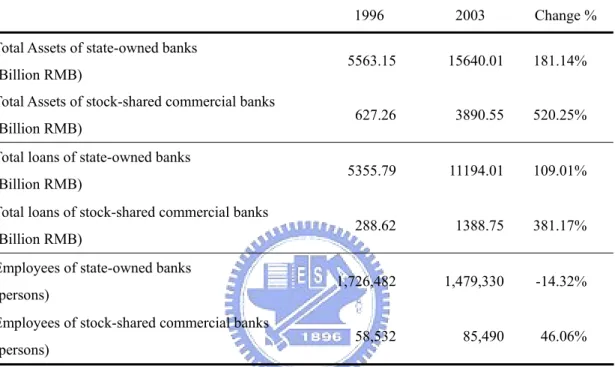
(11) allow foreign banks set up their branches in mainland China.. For the sake of surviving and. competing, China aggressively speeds her path to expand and reform.. The severely rising. growth of banking business can be addressed in Table 1 as below.. Table 1.. Business changes of the state-owned and stock-shared banks in China from 1996 to 2003 1996. Total Assets of state-owned banks (Billion RMB) Total Assets of stock-shared commercial banks (Billion RMB) Total loans of state-owned banks (Billion RMB) Total loans of stock-shared commercial banks (Billion RMB) Employees of state-owned banks (persons) Employees of stock-shared commercial banks (persons). 2003. Change %. 5563.15. 15640.01. 181.14%. 627.26. 3890.55. 520.25%. 5355.79. 11194.01. 109.01%. 288.62. 1388.75. 381.17%. 1,726,482. 1,479,330. -14.32%. 58,532. 85,490. 46.06%. Note: 1. Statistics are based on the Almanac of China’s Finance and Banking. 2. The monetary unit is People’s Currency (RMB) in billion.. In the year of 2003, the amounts of total assets of the state-owned banks are at 15640.01 billion People’s Currency (RMB), the 2.81 times of 1996.. The amounts of total assets of. stock-shared commercial banks are at 3890.55 billion RMB, the 6.20 times of 1996. The employees of stock-shared commercial banks increased 46% from 1996 to 2003; meanwhile, there was a 14% decline of staff of the state-owned banks.. The total loans also increase. 109% and 381% respectively during the same periods. It is obvious that these nationwide banks have a rapid and lots of growth in business operation, and the stock-shared commercial banks recruit more employees while the state-owned commercial banks cutback in personnel. This may imply that China is preparing to face the challenge. 3.

(12) Table 2.. The growth of investments, loans and deposits of banks from 1996 to 2003 Inv. / Dep.. L. / Dep.. (I+L) / D. Ratio. ratio. ratio. 60317.95. 0.073. 0.764. 0.837. 2482.24. 3551.13. 0.156. 0.699. 0.855. 3784.71. 48527.38. 63106.86. 0.060. 0.769. 0.829. Joint-equity banks. 567.64. 2672.68. 3931.29. 0.144. 0.680. 0.824. 1998 State-owned banks. 5506.26. 48754.86. 59513.39. 0.093. 0.819. 0.912. Joint-equity banks. 715.65. 2887.76. 4477.62. 0.160. 0.645. 0.805. 1999 State-owned banks. 6767.13. 51405.30. 75159.74. 0.090. 0.684. 0.774. Joint-equity banks. 731.44. 3044.67. 3487.59. 0.210. 0.873. 1.083. 11119.22. 47199.14. 76910.29. 0.145. 0.614. 0.758. 902.35. 3696.88. 4258.75. 0.212. 0.868. 1.080. 2001 State-owned banks. 15882.02. 51116.41. 63586.75. 0.250. 0.804. 1.054. Joint-equity banks. 1512.53. 4790.66. 6142.59. 0.246. 0.780. 1.026. 2002 State-owned banks. 17646.98. 53205.36. 66653.35. 0.265. 0.798. 1.063. Joint-equity banks. 1909.24. 5908.76. 7224.47. 0.264. 0.818. 1.082. 2003 State-owned banks. 18021.71. 55130.35. 67260.81. 0.268. 0.820. 1.088. Joint-equity banks. 2150.98. 6839.55. 8314.86. 0.259. 0.823. 1.081. Period. Ownership Type. Investments. Loans. Deposits. 1996 State-owned banks. 4421.41. 46062.56. Joint-equity banks. 552.97. 1997 State-owned banks. 2000 State-owned banks Joint-equity banks. Note: 1. Statistics are based on the Almanac of China’s Finance and Banking. 2. The monetary unit is People’s Currency (RMB) in billion.. Behind the aggressive growth and expansion of banking business, however, it seems that Chinese banks still operate in the old manner that is only to increase the volume of business without improving management.. Table 2 shows the growth of investments, loans and. deposits of nationwide banks in China.. A much higher loan-to-deposit ratio but a much. lower investment-to-deposit ratio means that these banks acquire deposits and then only issue loans obviously; they have poor ability to plan good investment projects to create more profits. This may be a reason for wasting inputs or causing inefficiency.. Besides a thorough review of banking industry in mainland China can bring a complete understanding of current status in Chinese financial market. 4. Taiwan also joined WTO in.

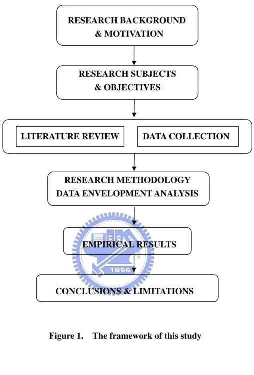
(13) 2001 and will face the same challenge of opening financial market, too.. It is quite indeed. necessary for Taiwanese banks to know earlier their opponents from China.. 1.3 Research objective Via a four-stage data envelopment analysis (DEA) approach proposed by Fried et al. (1999), this study measures Chinese bank efficiency and examines the influence from external factors to banks’ performance.. This approach separates the pure managerial inefficiency. caused by managers and inefficiency caused by operational environment from overall inefficiency. Previous efficiency analysis of banking institutions are numerous, but only very limited studies focused on the influence of the operational environment. The four-stage DEA application proposed by Fried et al. (1999) is as follows: The relative performance of each bank can be examined in the first stage; the significant external factors which are indeed influence the banks’ performance can be identified in the second stage; the overall inefficiency can be decomposed into the pure managerial inefficiency and the inefficiency due to operational environment in the final stage. Figure 1 illustrates the research framework of this study.. The reminder of this thesis is organized as follows: review.. Section Two is the literature. Section Three clearly describe the methodology adopted in this study. Section. Four presents the empirical findings and analysis. limitation of this study.. 5. Section Five is the conclusion and.

(14) RESEARCH BACKGROUND & MOTIVATION. RESEARCH SUBJECTS & OBJECTIVES. LITERATURE REVIEW. DATA COLLECTION. RESEARCH METHODOLOGY DATA ENVELOPMENT ANALYSIS. EMPIRICAL RESULTS. CONCLUSIONS & LIMITATIONS. Figure 1.. The framework of this study. 6.

(15) 2 Literature Review. 2.1 Literature review of Data Envelopment Analysis approach Farrell (1957) proposed that the efficiency of a firm consists of two components: technical efficiency and allocative efficiency. The former reflects the ability of a firm to obtain maximal output form a given set of inputs, and the later reflects the ability of a firm to use the inputs in optimal proportions. measure of total economic efficiency.. These two measures are combined to provide a. Based upon above propositions, Charnes et al. (1978). proposed a linear program model to minimize the total inputs under the given outputs. It is called as CCR model named by the alphabetical order of their last names.. Moreover, in their. paper, the term “data envelopment analysis; DEA” was first used.. The authors also. introduced a phrase “decision making unit; DMU” which represents the firm or unit that be observed or evaluated. This CCR model will be introduced in detail in Methodology.. Since the pioneering work by Charnes et al. (1978) introducing DEA approach, it has been used to assess comparative efficiencies of firms in a wide range, for example, in secondary schools (Smith and Mayston, 1987; Thanassoulis and Dunstan, 1994), police forces (Thanassoulis, 1995; Drake and Simper, 2005), farms (Thompson et al., 1990), public sector in local government (Worthington and Dollery, 2000); waste management (Worthington and Dollery, 2001), etc.. 2.2 Literature review of bank efficiency around the world Efficiency studies in finance and banking via DEA are also voluminous in recent years. Ayadi et al. (1998) attempted to determine the quality of bank management in Nigeria by 7.

(16) using DEA approach from 1991 to 1994.. Karim (2001) investigated the cost efficiency of. 155 banks from five ASEAN countries during the period from 1989 to 1996.. Krivonozhko. et al. (2002) made the efficiency analysis of 150 Russian banks in 1998, just after the banking default in Russia in the same year.. Pastor and Perez (2002) analyzed cost and profit. efficiency of banks in ten countries of the European Union during the period from 1993 to 1996.. Jemric and Vujcic (2002) evaluated bank efficiency in Croatia from 1996 to 2000 by. using the DEA approach.. Sathye (2003) measured the productive efficiency of banks in. India during the period from 1997 to 1998.. Ozkan-Gunay and Tektas (2006) measured the. technical efficiency of Turkish non-public banks from 1990 to 2001 via CCR DEA model.. Based upon the decomposition technical efficiency from pure technical efficiency and scale efficiency, Aly et al. (1990) utilized a nonparametric frontier approach to compute the overall, technical, allocative, and scale efficiency for a sample of 322 U.S. independent banks in 1986.. They took real estate loans, commercial and industrial loans, consumer loans, all. other loans and demand deposits as five outputs, labor, capital and loanable funds as three inputs and three price information of each input. Their empirical results indicated that their sample banks are characterized by relatively low level of overall efficiency, and these banks could produced the same level of output by using only 65% of the inputs actually used. Thus, inefficiency in these banks might be attributed to under-utilization or wasting of inputs. For the advanced analysis, the pooled sample banks were split into two sub-samples: banks that are allowed to operate branches (212) and those that are prohibited from operating branches (110) to test the null hypothesis that the two sub-sample banks were drawn from the same population (environment). Their null hypothesis could not be rejected in their study, which means the two sub-sample banks would face the same environment. Finally, they used multiple regression analysis to conclude that the diversity of financial products and bank. 8.

(17) location are significantly accounted for the inefficiency.. Huang (1997) conducted a translog cost function with three inputs (deposits, labor and capital) and three outputs (financial investment, short-term loans and long-term loans) to examine the cost efficiency of twenty-two banks in Taiwan from 1981 to 1992. In 1992, Taiwan regulatory government allowed the establishment of new stock-shared bank and its branches. Huang almost described clearly the process of bank evolution and the business operation of Taiwan’s banks, and his work is almost a complete review before the Taiwan’s financial opening in 1992.. The input-output variable specification and translog cost function. in his model are almost followed by later studies.. Seiford and Zhu (1999) examined the performance of the top fifty-five U.S. commercial banks via two production process which separates profitability and marketability. Their two-stage production is profit earning in the first stage and market value generating in the second stage.. Their sample banks were drawn from the Fortune 1000 (Fortune April 29,. 1996), ranking by revenue.. Their procedure is divided into two stages and eight factors are. expressed as inputs and outputs in each stage. The first stage measured profitability, i.e., a bank’s ability to generate the revenue and profit in terms of its labor, assets and capital in financial market.. The second stage measures marketability, i.e. a bank generates market. value, total returns to investors, and earnings per share in the stock market by profit and revenue. It can be seen that profit and revenue serve as mediator in bank production that they are the outputs from the first stage and the inputs to the second stage.. The efficiency of. both two stages is based on CCR DEA model. Their empirical findings indicated that close to 90% of the banks are inefficient in both profitability and marketability. Furthermore, most large banks exhibit better performance on profitability, whereas smaller banks tend to perform. 9.

(18) better with respect to marketability. This suggested that bank size may have a positive effect on profitability but negative effect on marketability.. With respect to the extended application of DEA measurement, Kao and Liu (2004) attempted to predict the performance of twenty-four commercial banks in Taiwan via CCR DEA model.. They claimed the insufficiency of prediction only by using financial ratios such. as ROE, EPS, P/E ratio, etc.. The prediction of the sample banks is based on their own. financial forecasts disclosed by themselves. The uncertain forecasts of financial data are presented in ranges (lower and upper bound), so the results of the prediction of the efficiency scores which are computed by interval data are also in ranges.. According to the comparison. of the results form their prediction and traditional financial ratios, a bank that had several financial poor ratios last year could obtain higher predicted efficiency scores next year. Therefore, the authors suggested that it is misleading to only use financial ratio analysis to examine, evaluate, and even to forecast the performance of a bank, especially in the financial environment with rapid changes and intense competition.. Wang et al. (2005) used nonparametric DEA models, including CCR, BCC, Bilateral, Slack-Based Measure and the FDH models, to evaluate the overall, pure and scale efficiencies of the sixteen nationwide commercial banks in mainland China.. The sixteen banks in China. are classified into two ownership groups: four state-owned banks and twelve stock-shared banks.. The authors used total capital and total assets as the two input variables, and net. profit, return on equity (ROE) and return on assets (ROA) as the three output variables. Their study concluded with three findings below: First, the FDH model analysis can not distinguish between efficient and inefficient banks from their sample banks; nevertheless, the CCR and BCC models can do. Second, seven banks is in the increasing returns-to-scale. 10.

(19) stage, which means that those banks can improve their performance by increasing their size, and the others are in the decreasing returns-to-scale stage.. Third, on average, the. stock-shared banks have higher efficiency than the state-owned banks do. However, the authors only took year 2004 as study period. incomplete results.. The neglect of panel data might cause. They either did not consider the environmental factors which influence. the performance directly and indirectly that it is not adequate to define the reason of inefficiency.. Cheng and Dran (2005) used stochastic frontier model to estimate the efficiency of nineteen major banks in China from 1998 to 2002.. With respect to the effect of exogenous. factors on bank’s inefficiency, they concluded that joining WTO is a positive force to improve the efficiency of China banking industry, however, the duration of establishment, the amount of total loans and the state-owned ownership are negative factors to account for the efficiency. It is suggested that the ownership reform to stock-shared type and decrease of total loans can improve the efficiency under the current circumstance.. Howland and Rowse (2006) used the DEA model to measure the efficiency of branches of a major Canadian bank to compare with the results of a U.S. bank studied by Golany and Storbeck (1999) during the same period.. With almost the same input and output variables,. the U.S. bank has higher averaged efficiency score; however, the score distribution of the Canadian bank is more central (with lower standard deviation of efficiency scores). The reason may be the sole regulatory supervision and banking regulation in Canada.. The. authors asserted that Canadian banks are more homogenous rather than U.S. banks.. Hu et al. (2006) investigated the efficiency of twelve nationwide banks in China from. 11.

(20) 1996 to 2003.. They used standard CRS and VRS DEA model to make the cost efficiency. analysis and seemingly unrelated regression model to examine the relation of external operational environment and banks’ performance.. Their empirical findings indicate as. follows: First, nationwide joint-equity commercial banks have significantly higher cost, overall technical, and scale efficiencies, but lower pure technical efficiency than state-owned specialized banks.. The next, a marginal increasing relation exists between the deposit-loan. ratio and cost efficiency and an inverted U-shape relation exists between the deposit-loan ratio and overall technical as well as scale efficiencies. Third, small-sized banks have higher cost and allocative efficiencies than large-sized banks do. Fourth, the twelve banks have lower cost efficiency after the 1997 Asian financial crisis and 2001 WTO participation, and they have lower overall technical, pure technical, and scale efficiencies after 2001.. Finally, the. twelve sample banks have significantly increasing overall technical and scale efficiencies from 1996 to 2003.. With respect to an attempt to further discussion on the relation of banks’ efficiency and their stock returns, Kirkwood and Nahm (2006) surveyed the cost efficiency of Austrian banks during the period from 1995 to 2002. Since the Austrian banking is dominated by four banks (the major banks), the authors utilized the VRS DEA model to compare the performance of the major banks and regional banks.. The authors used two datasets with the. same input components (employee, net fixed assets and interest-bearing liabilities) but the different output components (interest-bearing assets and non-interest income versus profit before tax) to investigate the banking service efficiency and their findings indicated that the major banks have better profit but poorer banking service efficiency. Based upon their computation of profit efficiency scores, the authors then used multiple regression, taking the excess return on stock (return on stock minus the risk free rate) as independent variable and. 12.

(21) taking excess market return and percentage change in profit efficiency as dependent variables, to test the significance of efficiency on stock return.. Efficiency changes of banks are fully. reflected in stock returns.. 2.3 Literature review of bank efficiency in China In order to be much closer to the real status of commercial banks recently in China, it is also necessary to review the papers which are studied by local researchers from mainland China to comprehend the empirical evidence from their studies with their own perspectives.. Chang (2003) utilized the basic DEA model and Malmquist Total Factor Productivity Index (Malmquist TFP Index) to make an overall analysis on efficiency of three types of commercial banks ( state-owned: 4, joint-equity: 10, city-owned: 37) in China from 1997 to 2001. Three inputs (capital, fixed assets and total expenditure) and three outputs (deposits, loans, and earnings before tax; EBT) were used in the study. The author also compared the results of original and adjusted technical efficiency by excluding bad loans from total loans to examine the effect of management.. The author concluded that the stock-shared banks have. higher relatively efficiency, and state-owned banks have a large amount of bad loans which indeed decreased the performance. Besides, the three types of banks presented an efficiency improvement from 1997 to 2001 according to Malmquist TFP Index analysis. Among the papers studied by local researchers in China, especially focused on banking efficiency analysis via DEA approach, Chang (2003) adopted more comparatively intact sample sizes and periods.. It is one of a few better studies.. Liu (2004) took two outputs (interest income and non- interest income) and three inputs (fixed assets, employment, and total expenditures) to evaluate technical, pure technical, and 13.

(22) scale efficiency of fifteen commercial banks in China during the period from 2000 to 2002. The fifteen sample banks were classified into two ownership types (state-owned and joint-equity) to compare the performance.. The author also classified five groups of the. sample banks by total assets to suggest that the most efficient scale of assets is 1001 to 3000 billion RMB dollars.. The conclusion that technical inefficiency results from the scale. inefficiency for both the state-owned and joint-equity banks was obtained.. The scale. inefficiency is more serious especially in state-owned commercial banks.. Li and He (2005) claimed the importance of the quality of loans to banks, thus they took the risk into consideration to measure the efficiency of fourteen commercial banks in China from 1998 to 2000. The two output variables were EBT and total loans.. The five input. variables were employment cost, total deposits, fixed assets, risk index, and return on assets (ROA).. The risk index was defined as the weighted average of the capital and allowance of. bad loans, because the allowance of bad loans was positively interrelated to capital, the ability to neutralize the risk. The authors finally concluded that the technical efficiency of the stock-shared banks is better than that of state-owned banks. The inefficiency results from pure technical inefficiency in state-owned banks, but from scale inefficiency in stock-shared banks.. Pong et al. (2005) measured the pure technical and scale efficiency of fourteen commercial banks in China.. They used the panel data consisted of three outputs (loans, EBT. and investment) and three inputs (total liability, employees and total expenditure) during the period of 1993 to 2003. They also transformed all nominal variables into real variables by the GDP deflators by using 1993 as base year. Their empirical findings claimed that the joint-equity banks had higher technical efficiency with lower standard deviation of efficiency. 14.

(23) scores before 1996, but the results turned opposite after 1997 to 2003.. Therefore, the. authors asserted that it is perhaps not necessary for state-owned commercial banks to wholly privatize to obtain higher efficient performance.. Mao (2006) used a DEA regression model to establish a production function of commercial banks in China via Cobb-Douglas production function. banks in the study.. There were fourteen. The author used three output variables (net income, loans, and deposits). and three input variables (capital, expenditures, and fixed assets) from 1995 to 2002.. The. empirical results indicated that the sole ownership held by government was the main reason causing lower efficiency.. Thus, the author clearly suggested that the joint-equity type is an. effective pattern of ownership reform for Chinese banking industry.. Among the studies focused on Chinese banking evaluation studied by Chinese local researchers, there are few ones took into account external factors which influenced performance of banks.. Zhu et al. (2004) utilized two-stage procedure to conduct an. advanced analysis on fourteen commercial banks’ efficiency from 2000 to 2001.. They. computed the efficiency scores via DEA model first, and then they examined the significance of environmental variables via Tobit regression to confirm the significant variables which indeed influenced the efficiency and / or inefficiency.. Their empirical findings indicated that. the stock-shared banks have higher efficiency scores than state-owned banks do, and the ROE, ownership type and location of the environmental factors do significantly account for the inefficiency.. Moreover, this study further suggested that the ownership reform for. state-owned commercial banks should be an optimal approach to improve these banks’ efficiency.. 15.

(24) 2.4 Literature review of efficiency focused on environment-adjusted analysis Previous study on the external operational environment and measures of efficiency based on DEA model can be broadly classified into two categories: the all-in-one approach and the two-stage approach.. The all-in-one approach first proposed by Charnes et al. (1981) includes the external operational environment variables directly in the linear programming (LP) formulation along with the traditional inputs and outputs. The external factors which are from the operational environment and indeed influence the firms’ performance are treated as the additional inputs and outputs along with the real inputs and outputs in the same LP formulation to analyze. However, an additional input and output variables from external factors could wrongly estimate the real efficiency.. If the operational environment enters the LP formulation as an. input, this implies that more outputs could be produced, suggesting that the operational environment is favorable.. If the operational environment enters the LP formulation as an. output, this implies that more inputs are required, suggesting that the operational environment is unfavorable. This prior input or output classification is unsuitable if such external factors can not be classified appropriately, e.g. age, gender, vocation, education background, etc.. It. may make little sense for an external feature of the operational environment.. The two-stage approach called by Coelli et al. (1998) includes the traditional inputs and outputs in the LP formulation used to compute efficiency, which is then used as the dependent variable in a second stage regression, where the explanatory variables measure the external environment.. An advantage of the two-stage approach is that the influence of the external. variables on the production process can be tested in terms of both sign and significance. However, a disadvantage is that the two-stage approach ignores the information contained in 16.

(25) the slacks and surpluses from inputs and outputs. This may bias the parameter estimates and give misleading conclusions regarding the impact of each external variable on efficiency. The two-stage procedure does not provide a separate measure of managerial efficiency or inefficiency.. Fried et al. (1999) introduced a four-stage DEA approach to estimate the influence by the environment-adjusted variables of American hospital-affiliated nursing homes in 1993. They used two outputs: inpatient days of skilled care and inpatient days of intermediate cares, and four inputs: registered nurses, licensed practical nurses, other personnel, and non-payroll expenses. As suggested by Fried et al., the four-stage DEA approach has some intriguing findings:. First, it uses the information contained in the slacks or surpluses of the original. model. Second, it does not require imposing a sign on the effect of an external variable on inefficiency. Third, it provides tests of significance of each external variable on inefficiency in each individual input (for an input-oriented model) or output dimension (for an output-oriented model). variable.. Fourth, it provides an overall effect on inefficiency for a categorical. Finally, it can generate a single result of firms’ inefficiency caused by managers.. The utilization of the four-stage DEA procedure can avoid the above disadvantages of the all-in-one approach and the two-stage approach.. As suggested by Fried et al., this. approach is not necessary to classified the external variables into additional input and output categories prior to the analysis, and information on slacks or surpluses generated by the initial model is used in the calculations. The result would rely on the conventional DEA model and efficiency estimation theory, and the influence of the external variables on each input variables can be tested. The management component of inefficiency also could be separated from the influences of the external operational environment.. 17. This approach is adopted in.

(26) this study.. Pastor (2002) also proposed his new three-stage sequence based on DEA model to evaluate the efficiency of banks in Spain, Italy, France and Germany from 1988 to 1994. The main concept of his procedure is to find out some factors out of business operation.. The. external factors would indeed affect the performance of banks. The author considered that the most important of those external factors is risk which mostly results from bad loans, caused by poor management.. The total bad loans were decomposed into two components:. one due to poor risk management and another due to external economic and environmental factors.. The author then compared the results by controlling the bad loans to compute the. efficiency scores via DEA.. The conclusion indicated that the external factors do not account. for the inefficiency significantly, but the bad loans caused by failed risk management do. Although it may be much simple to define risk only as bad loans.. However, the concept that. separating inefficiency from managerial failure and unavoidable external factors is worthy being noticed.. Based on Fried et al. (1999), Drake and Simper (2005) and Drake et al. (2006) extended the application of the four-stage DEA procedure to respectively analyze the efficiency of United Kingdom police force and Hong Kong banking institutions excluding the influence of external environment.. Drake and Simper (2005) compare the results from police force efficiency measured by DEA and by radar approach, the wholly output based measurement, currently advocated by Home Office in the United Kingdom as a new police force performance evaluation.. The. performance radar approach took multiple criteria used to evaluate each regional police force. 18.

(27) into consideration simultaneously such as numbers of reducing crimes, numbers of the criminal offenders brought to justice, promoting level of public safety, citizen satisfaction and resource usage.. Because the environment may be a penalty or benefit to an individual unit. that is under the evaluation, the authors attempted to purge the raw DEA scores of any impact from environmental factors outside the control of individual police force by using the slack-based environment adjusted input specification. In order to ensure the environmental factors are indeed adequately accounted for, the authors used Tobit regression to determine the external variables, and then they could measure the inefficiency excluding the influence of environment.. More significantly, the authors claimed that the current radar approach. advocated by Home Office of UK could produce misleading assessments of the performance of individual police force, because the radar approach assumes each police force is in the same environment.. Using four-stage DEA approach proposed by Fried et al. (1999) helps to. exclude the external factors for all police force, thus all police can be evaluated equally.. Drake et al. (2006) also assessed the relative technical efficiency of banking institutions operational in the Hong Kong financial market from 1995 to 2001.. They used the panel data. sample consisted of 413 observations to almost follow the four-stage DEA approach introduced by Fried et al. (1999), using a profit-oriented specification with revenue components as outputs and cost components as inputs.. Therefore, the three inputs variables. specified are employee expenses, other non-interest expense and loan loss provisions, and the three output variables specified are net interest income, net commission income and total other income.. They also adopted the intermediation specification (with employees, capital,. deposits as inputs and investment and loan as outputs) to assess the technical efficiency to compare the results via profit-oriented specification.. Their conclusive results indicated quite. clearly that the failure to incorporate slacks formally and directly into the efficiency analysis. 19.

(28) could sometimes produce inflated and misleading indications of relative efficiency, even though the rank correlation between the two sets of results is relatively high.. 2.5 A brief summary of the literature reviews The existing studies applying the DEA model to compute bank efficiency are voluminous.. Research objects include those in the ASEAN economies (Karim, 2001),. Australia (Kirkwood and Nahm, 2006), Canada (Howland and Rowse, 2006), Croatia (Jemric and Vujcic, 2002), European Union (Pastor and Perez, 2002), Russia (Krivonozhko et al., 2002), U.S. (Aly et al., 1990; Seiford and Zhu, 1999), etc. studies focused on the banking industry in China.. However, there are only few. Some local Chinese researchers try to. begin investigating the performance of the banking institutions in China. They conclude that joint-equity commercial banks are more efficient rather than state-owned banks. However, these existing Chinese articles (such as Chang, 2003; Liu, 2004; Li and He, 2005; Mao, 2006; etc.) usually do not incorporate exogenous factors into efficiency computation.. The. computed efficiency scores will hence be distorted by neglecting exogenous variables such as ownership, establishment duration, bank size, etc.. A bank may get a lower efficiency score. because of unfavorable environment, making the efficiency comparison unfair. This study applies Fried et al. (1999) to obtain the environment-adjusted efficiency.. 20.

(29) 3. Methodology. 3.1 Theory of banking evaluation and variable definition The estimation of bank efficiency rests on appropriate definitions and certain assumptions regarding the measurement of variables.. Choosing the inappropriate variables. may lead the incorrect evaluation and conclusion. Sealey and Lindley (1977) provided a concrete theory of financial firm evaluation.. In order to develop a measurement model of. financial firm behavior, the authors make a complete analysis of production and cost conditions and define inputs and outputs carefully.. In their point of view, the technical. process of production for financial firms is a process of transformation.. Here transformation. implies that certain goods and /or services enter into a process in which they lose their existence in the original form while other goods or services are generated.. Thus a. transformation process of a financial firm can be further analyzed by its operational behavior. For commercial banks, the transformation process involves the borrowing of funds from surplus units and lending those funds to deficit units.. Banks acquire deposit funds by paying. interest expenses, and then they make investments and issue loans to earn incomes. This is the standard and ordinary behavior of commercial banks.. Based upon the behavior theory of Sealey and Lindley (1977), Berger et al. (1987) further proposed two evaluation perspectives of financial firms: production versus intermediation approach.. Under the production approach, banks produce accounts of various. sizes by processing deposits and loans and incurring capital and labor costs.. Therefore, the. numbers of accounts of deposits and loans are regarded as outputs while fixed assets and labor costs regarded as inputs. Under the intermediation approach, however, banks intermediate deposited and purchased funds into loans and other investment assets, so the loans and 21.

(30) investments are outputs and deposits, employee and total fixed assets are inputs.. The. authors deemed that the intermediation approach is more appropriate in the evaluation model for commercial banks. Because incorporating the quantity of accounts for investment, loans and deposits into the output specification under the production approach means each account have the same weight. This may bias the importance of each transaction.. Consequently,. Berger and Humphrey (1991) further took the intermediation approach to measure the inefficiency for U.S. banks.. In order to evaluate the efficiency of transformation process, the. intermediation approach is adopted in this study.. 3.2 CRS models of Data Envelopment Analysis Data envelopment analysis involves the use of linear programming methods to construct a non-parametric piece-wise surface over the data.. Efficiency measures are then computed. relative to this surface. Farrell (1957) proposed the piece-wise linear convex approach to frontier estimation, but only a few authors over the next two decades followed his paper. Boles (1966) and Afrait (1972) advised mathematical programming methods which could achieve the task, but not achieve very wide attention until Charnes et al. (1978). Similar reviews of the methodology are presented by Seiford and Thrall (1990) and Seiford (1996). There are now a large amount of papers that have extended and applied the DEA methodology.. Charnes et al. (1978) proposed a constant-returns-to-scale (CRS) model with an input orientation, also called as CCR model in alphabetic order of their last names.. In the. input-orientated CRS DEA model, there are data on N inputs and M outputs for each of K firms.. For a certain i-th firm, these are represented by the column vectors x i and y i .. The N×K input matrix X and the M×K output matrix Y represent the data for all K firms. 22.

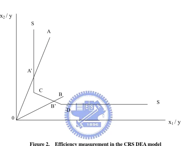
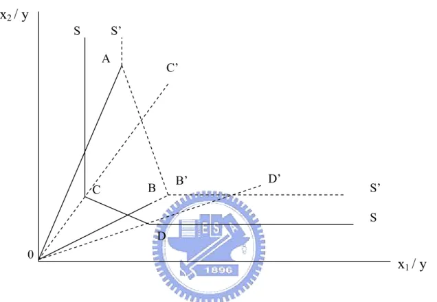
(31) The input-oriented CRS DEA model then solves the following linear programming problem for firm i in each year:. min θ ,. (1). θ ,λ. s.t. - yi + Y λ ≥ 0,. θ xi - X λ ≥ 0, λ ≥ 0.. where θ is scalar and λ is a K×1 vector of constants.. The value of θ obtained will be the efficiency score for the i-th firm lies in between 0 and 1.. According to the definition of Farrell’s (1957), the value of unity indicates a point on. the frontier and hence a technically efficient firm.. The DEA problem in equation (1) takes. the i-th firm and then seeks to radially contract the input vector, xi, as much as possible, while still remaining within the feasible input set.. The inner-boundary of this set determined by. the observed data points is a piece-wise linear iso-quant. The radial contraction of the input vector, xi, produces the projected point, (Xλ, Yλ), on the frontier of this technology. This projected point is a linear combination of these observed data points.. The constraints in. equation (1) confirm that this projected point cannot lie outside the feasible set. Figure 2 illustrated the efficiency measurement, that C and D are the efficient firms which define the frontier such that A and B are inefficient firms. Farrell’s (1957) measure of overall technical efficiency (OTE) explains the efficiency of firms A and B as OA' / OA and OB' / OB , respectively.. As illustrated in Figure 2, SS is the frontier of efficiency. Since firm A could reduce inputs from A to A’ to be efficient, AA ' is hence known as the radial slack in literature. The 23.

(32) difference form A’ and C is called the non-radial slack. The total slack of an input is equal to radial slack plus non-radial slack. The slacks can be treated as the wasting level of input resources.. x2 / y S A. A’. C. B B’. S D. 0. x1 / y. Figure 2.. Efficiency measurement in the CRS DEA model. An input-oriented DEA model is to solve the input minimization problem under a given output level, however, an output-oriented DEA model is to solve the output maximization problem under a given input level instead.. Most general industries are suited to use. input-orientated model because firms can decide their input resources according to their own budgets. Thus, the input-oriented DEA model is the primary for use. This study also adopted the input-oriented DEA model. There are still a few cases using the output-oriented model that the firms may be given a fixed quantity of resources and asked to produce as much output as possible. The output orientation is more appropriate for a public sector of a government, for example, just like waste recycle or garbage to dispose. 24.

(33) 3.3 Four-stage DEA approach. Fried et al. (1999) used a slack-based measure, the four-stage DEA procedure, to estimate the influence by the environment-adjusted variables of American hospital-affiliated nursing homes in 1993. They believed that the characteristics of the external environment could influence the ability of management to transform input to output. This procedure for incorporating the operational environment into a measure of technical efficiency can obtain a separate measure of managerial inefficiency.. As introduced by Fried et al. (1999), the first stage is to compute a DEA frontier by using the traditional inputs and outputs according to DEA model theory.. The external. variables are excluded. The efficiency scores as well as input slacks and output surpluses are computed for each observation.. In the second stage, a system of equations is specified in which the dependent variable for each equation is the sum of radial and non-radial input slack for an input-oriented model or radial plus non-radial output surplus for an output-oriented model. The independent variables are used to measure the features of the external operational environment. This equation system identifies the variation in total measures of inefficiency attributable to factors outside the control of management.. The third stage is to use the parameter estimates from the second stage to predict the total input slack or output surplus, depending upon model orientation. These predicted values represent the ‘allowable’ slack or surplus, due to the operational environment, and are used to compute adjusted values for the primary inputs or outputs.. 25.

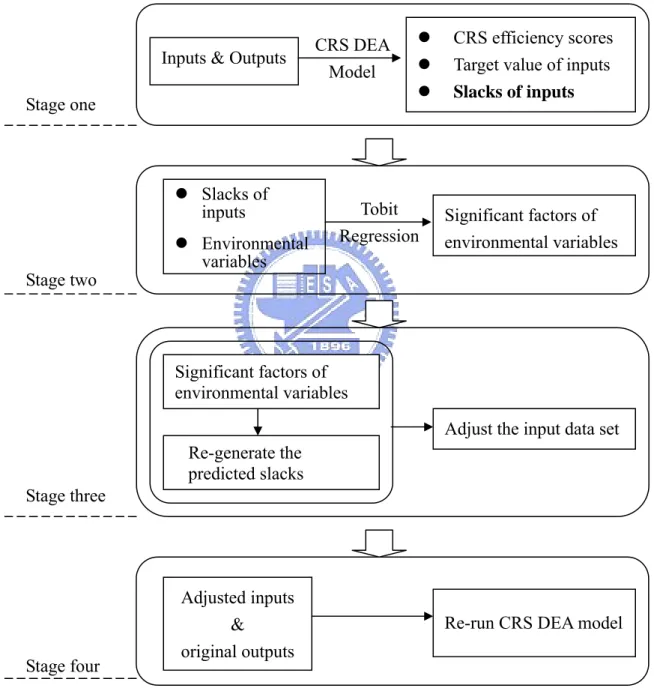
(34) The fourth stage is to re-run the DEA model under the initial output specification by using the adjusted input data set.. The new radial efficiency measures incorporate the. influences of the external variables into the production process, and isolate the managerial component of inefficiency. Figure 3 illustrates the four-stage DEA procedure.. Inputs & Outputs. CRS DEA Model. Stage one. z Slacks of inputs. Stage two. z Environmental variables. z z z. Tobit Regression. CRS efficiency scores Target value of inputs Slacks of inputs. Significant factors of environmental variables. Significant factors of environmental variables Adjust the input data set Re-generate the predicted slacks Stage three. Stage four. Adjusted inputs & original outputs. Re-run CRS DEA model. Figure 3. Illustration of four-stage procedure. 26.

(35) The detail of the procedure is disclosed as below.. The first stage begins with a specification of production technology. The efficiency. scores, the value of θ in equation (1), and the target value of the input variables during the sample period for each firm are computed by using the CRS DEA model. The definition of input target value is an input level which is utilized by a firm to be efficient.. The second stage is to estimate the N input equations by using Tobit regression because. of the estimative range from zero to infinity.. The dependent variables are radial plus. non-radial input slack equal to the absolute value of input actual value minus input target value.. The independent variables are measures of external conditions applicable to the. particular input.. The objective is to quantify the effect of external conditions on the. excessive use of inputs. The N equations are specified as:. IS it j = f j ( Z it j , β tj , ε tj ). (2) i = 1 ,......,K ; j = 1 ,......,N ; t = 1 ,......,T ;. where IS it j is the total radial plus non-radial slack of input j for firm i in time t based on the DEA results from stage 1, Z it j is a vector of variables characterizing the operational environment for firm i that may affect the utilization of input j , β tj is a vector of coefficients to be estimated; and ε tj is a disturbance term. These equations explain the variation in total by-variable measures of inefficiency. Note that the explanatory variables characterizing the operational environment in equation (2) are not restricted to be the same. 27.

(36) across equations, needing not have a linear relationship with the dependent variables and can be a mixture of continuous and categorical variables.. The output surplus in this stage for an input oriented model is omitted. As Fried et al. (1999) mentioned, “An input oriented model takes output as given and measures inefficiency by the potential reduction in inputs. Output surplus exists in empirical applications because the data set is sparse for some output vectors.. Where it does exist, it is likely to be. composed mostly of zeros and have insufficient variation to be useful in the estimation.”. The third stage is to use the estimated coefficients from the regression to predict total. input slack for each input and for each unit based on its external variables: ∧ t. ∧ t. (3). IS i j = f j ( Z it j , β j ). i = 1 ,......,K ; j = 1 ,......,N ; t = 1 ,......,T ;. As proposed by Fried et al. (1999), the predictions are used to adjust the primary input data for each unit. The each adjusted input data of each input for each sample firm is the original input plus the difference between maximum predicted slack and predicted slack as equation (4) below:. ∧ t. ∧ t. (4). X it j adjusted = X it j + [ Max{IS j } − IS i j ] i = 1 ,......,K ; j = 1 ,......,N ; t = 1 ,......,T ;. 28.

(37) ∧ t. where Max{IS j } means the maximum predicted slack of the firms for input j in the same sample year t. The purpose of adjusting the primary input data by the difference between maximum predicted slack and predicted slack is to establish a base equal to the least favorable set of external conditions. A firm with the maximum predicted slack means it would get the most severe penalty by the operational environment. The environment where a firm with the maximum predicted slack operates in is the least favorable external environment. According to equation (4), this firm would not have to adjust its inputs at all. A firm with external variables generating a lower level of predicted slack would have its input vector adjusted to put it on the same basis as the firm with the least favorable external environment. The reason why choosing to use the least favorable operational environment as the base is to provide a performance target that managers can attain regardless of their operational environment.. Managers will have no excuse of operational environment for failing to. achieve the performance target.. A special attention must be paid that the input adjustment takes the form of an increase in the original input. Predicted slack below the maximum predicted slack is attributable to external conditions more favorable than the least favorable conditions prevailing in the sample for that input. The purpose of the adjustment is to penalize the firm for the fewer inputs required to operate under favorable external conditions. Besides, another advantage is to avoid the possibility of a negative value for an adjusted input from the estimation of the Tobit regression, rendering the DEA problem for that unit without a solution. By increasing the input vector and leaving the output vector unchanged, the firm's performance is purged of the external advantage.. This makes it possible to isolate managerial inefficiency by. re-running the DEA model on the adjusted data set.. 29.

(38) The final stage is to use the adjusted data set to re-run the DEA model under the initial. input-output specification and generate new radial measures of inefficiency. These radial scores measure the inefficiency that is attributable to management.. x2 / y S’. S A. C. C’. D’. B’. B. S’ S. D 0. Figure 4.. x1 / y. Shift in frontier after the slack-based adjustment in the CRS DEA model. Figure 4 illustrates the shifting course of frontier after conducting the slack-based adjustment in the CRS DEA model. Firm A with the maximum predicted slacks would get the most severe penalty by the operational environment. After conducting the slack-based adjustment in stage two and three, firm A would have the minimum adjustment (zero) while firm B would be added a punished input vector matrix from B to B’, and so do C and D to C’ and D’ respectively. The benefit from the operational environment of each firm would be eliminated. All firms would be brought into the same operational environment, the least favorable environment, to be evaluated. After re-running the DEA model in stage four, the frontier of efficiency would shift from SS to S’S’. 30.

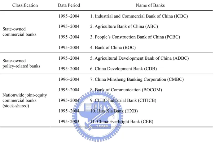
(39) 3.4 Tobit regression model. In a regression model, a dependent variable with the property that it has a discrete jump at any other threshold value is known as a limited dependent variable. The dependent variables of the second stage in this study are slacks of each input variable that have a discrete range form zero to infinity. It is indeed required for the unbiasedness of estimates. A regression model of the limited dependent variable adopted in this study is referred to as Tobit model which is proposed by Tobin (1958).. Tobit regression model adopted in this study is below:. ∧ t. ∧ t. C j + β j Z ijt + ε tj if. IS ij > 0 or. 0,. IS ij ≤ 0 or. IS ij =. if. ∧ t. ε tj < - C j - β j Z ijt ε tj ≥ - C j - β j Z ijt. (5). 3.5 Data (1) Sample banks. There are eleven banks as Table 3 shown in this study: four state-owned commercial banks, two state policy-related banks, and five nationwide joint-equity commercial banks. All eleven sample banks are nationwide because their branches are around China. This study uses panel data from 1995 to 2004, including two outputs and three inputs, to investigate the technical efficiency of eleven banks based on the CRS DEA model. Because of the missing and unavailable data in the Almanac of China’s Finance and Banking during the sample period, the panel data sample consists of 108 observations over the ten years. There are only ten banks in 1995 (China Minsheng Banking Corporation is excluded) and 31.

(40) 2004 (China Everbright Bank is excluded), meanwhile, eleven banks are in other years. Table 3 shows the classification and names of these sample banks in this study.. Table 3.. Classification and names of sample banks. Classification. State-owned commercial banks. State-owned policy-related banks. Nationwide joint-equity commercial banks (stock-shared). Data Period. Name of Banks. 1995~2004. 1. Industrial and Commercial Bank of China (ICBC). 1995~2004. 2. Agriculture Bank of China (ABC). 1995~2004. 3. People’s Construction Bank of China (PCBC). 1995~2004. 4. Bank of China (BOC). 1995~2004. 5. Agricultural Development Bank of China (ADBC). 1995~2004. 6. China Development Bank (CDB). 1996~2004. 7. China Minsheng Banking Corporation (CMBC). 1995~2004. 8. Bank of Communication (BOCOM). 1995~2004. 9. CITIC Industrial Bank (CITICB). 1995~2004. 10. Hua Xia Bank (HXB). 1995~2003. 11. China Everbright Bank (CEB). (2) Output and input variables. Based on the intermediation specification, the two output variables in this study are investment (Y1) and loan (Y2), and the three input variables are deposit (X1), number of employees (X2), and net fixed assets (X3). All numerical data are compiled from the balance sheets, income statements, and employment calculation that are disclosed in the Almanac of China’s Finance and Banking from 1996 to 2005.. All nominal variables have been. transformed into real variables by the GDP deflators by using 1995 as the base year.. For outputs, investment (Y 1 ) is defined by the items of long-term, short-term, and securities investments shown in the balance sheets as assets of each bank. 32. Loan (Y 2 ).

(41) represents the net loans equal to total loans minus default loans and allowance of bad loans, also shown in the balance sheets of each bank.. For inputs, deposit (X1) is the amount of every deposit and the loans from other banks. The number of Employees (X2) is the total number of full-time employees in a bank. Net fixed assets (X3) is the difference of fixed assets minus accumulated depreciation of fixed assets.. All data above can be gathered from the financial statements and employment calculation in the Almanac of China’s Finance and Banking from 1996 to 2005.. (3) Environmental variables. Seven environmental variables that regressed on Tobit regression are used to predict the total slacks of the three input variables. These environmental variables are defined as below:. a. Duration (DUR):. It represents the establishment duration of a bank and is. computed from the year when its license was issued by the PBC to the year 2004.. b. Ownership (SHARE): This is a dummy variable which represents the ownership type of the sample banks. These banks can be categorized to two nationwide banks: state-owned specialized banks (commercial and policy-related banks) and joint-equity commercial banks.. The nationwide joint-equity commercial banks. belong to the share-allocation system, but the state-owned commercial and policy-related banks do not. The joint-equity commercial banks can be represented by SHARE = 1 and the state-owned banks can be represented by SHARE = 0. 33.

(42) c. Policy-related specialization (POLICY):. This is also a dummy variable.. The. policy-related banks sometimes have the mission and responsibility to carry out the financial policy made by PBC as Central Bank of China. In order to investigate the significant difference on performance between ordinary commercial and policy-related banks, this dummy variable is utilized.. Therefore, the two. policy-related banks in this study can be represented by POLICY = 1, while the other commercial banks are represented by POLICY = 0.. d. Deposit-loan ratio (DLR): This ratio represents the proportion of loans to deposits. According to the balance sheet of the eleven banks from 1995 to 2004 in the Almanac of China’s Finance and Banking, each bank’s deposit-loan ratio for the ten-year period (nine years for China Minsheng Banking Corporation and China Everbright Bank) can be computed after deflating by GDP price as the base year of 1995 followed the equation (6):. Deposit-loan ratio (DLR) = total loans / total deposits. (6). e. Bank size (SIZE): This is also a dummy variable which is used to investigate the relation of bank size and operational performance. According to the balance sheets of the eleven banks in the Almanac of China’s Finance and Banking from 1995 to 2004, the calculation of total assets of each bank is made by GDP deflator as the base year of 1995. It is then classified these eleven banks into two groups. The dummy variable, SIZE = 0, represents those banks whose average assets are over five hundred billions RMB each year. Otherwise, SIZE = 1 represents those banks whose total assets are under five hundred billions RMB each year. Using five hundred billions RMB as cut-off value can almost equalize each sub-sample size.. 34.

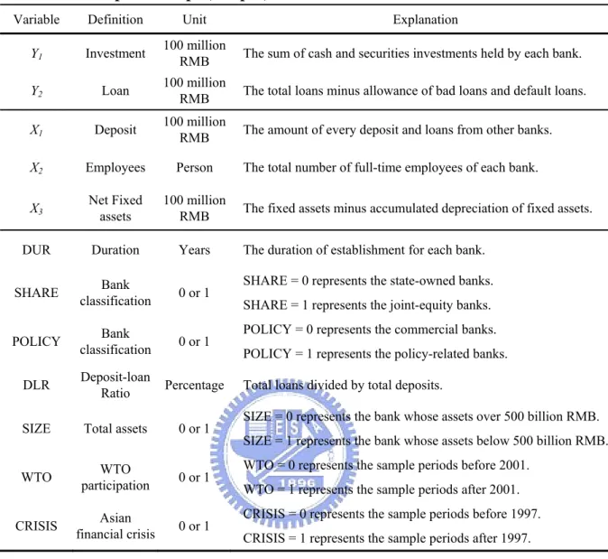
(43) f. WTO participation (WTO): The dummy variable WTO = 0 represents the period before China entered the World Trade Organization in 2001. The dummy variable WTO = 1 represents the period after China entered the World Trade Organization. This is in order to check if the inputs are more / less before and after participating WTO.. g. Asian financial crisis (CRISIS): The dummy variable CRISIS = 0 represents the period before the 1997 Asian financial crisis, and the dummy variable CRISIS = 1 represents the period after the 1997 Asian financial crisis. This is in order to check if the inputs are more / less before and after the 1997 Asian financial crisis.. The definition and description of these variables are as depicted in Table 4. The descriptive statistics of input and output variables are listed in Table 5. Table 6 shows that all relation between an input and an output satisfies the isotonicity property in which an output should not decrease with an increase in an input. All input and output variables are appropriately used for the sample banks to be evaluated.. 35.

(44) Table 4.. Description of input, output, and environmental variables. Variable. Definition. Unit. Y1. Investment. 100 million RMB. The sum of cash and securities investments held by each bank.. Y2. Loan. 100 million RMB. The total loans minus allowance of bad loans and default loans.. X1. Deposit. 100 million RMB. The amount of every deposit and loans from other banks.. X2. Employees. Person. X3. Net Fixed assets. 100 million RMB. DUR. Duration. Years. SHARE. Bank classification. 0 or 1. POLICY. Bank classification. 0 or 1. DLR. Deposit-loan Ratio. Percentage. SIZE. Total assets. 0 or 1. WTO. WTO participation. 0 or 1. CRISIS. Asian financial crisis. 0 or 1. Table 5.. Explanation. The total number of full-time employees of each bank. The fixed assets minus accumulated depreciation of fixed assets. The duration of establishment for each bank. SHARE = 0 represents the state-owned banks. SHARE = 1 represents the joint-equity banks. POLICY = 0 represents the commercial banks. POLICY = 1 represents the policy-related banks. Total loans divided by total deposits. SIZE = 0 represents the bank whose assets over 500 billion RMB. SIZE = 1 represents the bank whose assets below 500 billion RMB. WTO = 0 represents the sample periods before 2001. WTO = 1 represents the sample periods after 2001. CRISIS = 0 represents the sample periods before 1997. CRISIS = 1 represents the sample periods after 1997.. Descriptive statistics of input and output variables N. Minimum. Maximum. Mean. Std. Deviation. Investment. (Y1). 108. 0.30. 5761.99. 1077.37. 1572.30. Loans. (Y2). 108. 5.90. 17199.44. 4970.97. 5082.52. Deposits. (X1). 108. 7.31. 27666.40. 6603.62. 7883.88. Employees. (X2). 108. 487.00. 569983.00. 153383.85. 198296.01. Fixed Assets. (X3). 108. 0.26. 2163.27. 152.58. 250.38. Note: The monetary unit is at 100 Million RMB. 36.

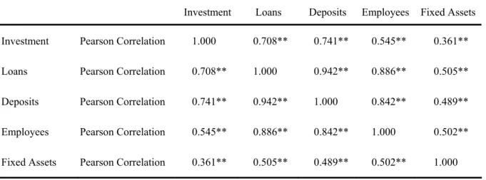
(45) Table 6.. Pearson correlations of inputs and outputs Investment. Loans. Deposits. Employees. Fixed Assets. Investment. Pearson Correlation. 1.000. 0.708**. 0.741**. 0.545**. 0.361**. Loans. Pearson Correlation. 0.708**. 1.000. 0.942**. 0.886**. 0.505**. Deposits. Pearson Correlation. 0.741**. 0.942**. 1.000. 0.842**. 0.489**. Employees. Pearson Correlation. 0.545**. 0.886**. 0.842**. 1.000. 0.502**. Fixed Assets. Pearson Correlation. 0.361**. 0.505**. 0.489**. 0.502**. 1.000. Note: ** represents significance at the 0.01 level.. 37.

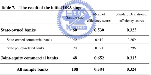
(46) 4. Empirical Results. 4.1 Stage one: Initial DEA. The CRS DEA model in this study includes two outputs and three inputs. The input and output variables are followed by the intermediation approach introduced by Berger et al. (1987).. Efficiency scores are computed by using an input-oriented setting.. Table 7. illustrates the initial DEA results. The average efficiency score is 0.584; i.e., on average, a bank could produce the same level of outputs with only 58.4 percent of the current inputs; or it could reduce the current inputs by 41.6 percent to perform its best.. Table 7.. The result of the initial DEA stage Mean of. Standard Deviation of. efficiency scores. efficiency scores. 60. 0.530. 0.325. State-owned commercial banks. 40. 0.410. 0.269. State policy-related banks. 20. 0.771. 0.296. 48. 0.652. 0.313. 108. 0.584. 0.324. Sample size. State-owned banks. Joint-equity commercial banks All sample banks. The policy-related banks have the best efficiency (average efficiency score at 0.771), and the joint-equity banks have the second best efficiency (average efficiency score at 0.652). The state-owned commercial banks are the worst (average efficiency score at 0.410). China Minsheng Banking Corporation has the relative higher performance. Agricultural Bank of China and China Construction Bank have the relative worse performance.. A simple. proposition that the nationwide joint-equity commercial banks have more efficient 38.

(47) performance than the state-owned banks do can be obtained.. It is particularly noteworthy that state-owned commercial banks have relative much larger slack value of each input. As depicted in Table 8, state-owned commercial banks’ average slacks of deposit, employees and net fixed assets are 18.08, 45.39 and 31.28 times of nationwide joint-equity commercial banks’ respectively.. Input slack, the absolute value. equal to the difference from actual and theoretical input, represents the wasting level of resource inputted. Especially in the input of number of employees, the average slack is at 297260.38, which means that there are 297260.38 redundant personnel for each state-owned commercial bank a year on average, the 45.39 times of joint-equity commercial banks. This is because that the state-owned banks carry the responsibility to ensure job security of each staff to earn his life under the socialism in China. The redundant personnel should be the main reason accounted for the inefficiency for state-owned commercial banks.. Table. 8. The average slacks of inputs from 1995 to 2004 Slacks of X1. State-owned commercial banks. Slacks of X2. Slacks of X3. 9867.02. 297260.38. 215.45. State-owned policy-related banks. 560.65. 12358.00. 20.90. Nationwide joint-equity banks. 545.74. 6549.12. 6.77. However, the initial DEA model does not provide a good measure of managerial performance. This too simple original DEA procedure will ignore the effect of environment where the banks operate in. It is possible that the real good performers who operate in an unfavorable external environment would be penalized, whereas the real poor performers who operate in a favorable external environment would be rewarded. 39.