使用Fuzzy Q-learning達成具公平性動態頻寬分配的MPLS-TP環

(1)

國

立

交

通

大

學

電機學院通訊與網路科技產業研發碩士班

碩

士

論

文

使用 Fuzzy Q-learning 達成

具公平性動態頻寬分配的 MPLS-TP 環

Dynamic Bandwidth Allocation with Fairness

by Using Fuzzy Q-learning for MPLS-TP Ring

研究生：陳俊魁

指導教授：張仲儒教授

(2)

使用 Fuzzy Q-learning 達成具公平性動態頻寬分配的 MPLS-TP 環

Dynamic Bandwidth Allocation with Fairness

by Using Fuzzy Q-learning for MPLS-TP Ring

研究生：陳俊魁

Student：Chun-Kuei Chen

指導教授：張仲儒

Advisor：Chung-Ju Chang

國立交通大學

電機學院通訊與網路科技產業研發碩士班

碩士論文

A Thesis

Submitted to College of Electrical and Computer Engineering National Chiao Tung University

in partial Fulfillment of the Requirements for the Degree of

Master in

Industrial Technology R & D Master Program on Communication Engineering

August 2011

Hsinchu, Taiwan, Republic of China

(3)

使用 Fuzzy Q-learning 達成具公平性動態頻

寬分配的 MPLS-TP 環

研究生：陳俊魁指導教授：張仲儒

國立交通大學電機學產業研發碩士班

摘要

近年來隨著行動上網的普及，資料形態的訊務需求日漸成長。由於消費大眾期待行動服務的收費價格能夠更低廉，電信營運商勢必在擴展網路的同時，必須兼顧降低成本支出。因此乙太網路技術夾帶著低價高效率的優勢，應用範圍逐漸從近端區域網路擴展到都會型區域網路。在使用乙太網路服務做傳輸媒介之上，提供各式功能的封包傳輸型網路之中，MPLS-TP 可以支援現有各式標準的服務保證機制，且具有虛擬鏈路及保護的功能。本篇論文將以提供公平性的篇刊分配在環狀網路中為基礎，考量了現實傳輸網路中，可用頻寬為隨時間動態變化的情況。傳統的 fair rate 機制所面對的震盪現象，將導入 fuzzy Q-learning 的機制進行改善，並以差異速率作為回授訊號之用。在模擬結果中可顯示，本文提出的 fair rate 產生器，將可有效改善 MPLT-TP 環的效能，包含降低收斂時間及提高整體網路頻寬使用效率。

(4)

Dynamic Bandwidth Allocation with Fairness by

Using Fuzzy Q-learning for MPLS-TP Ring

Student: Chun-Kuei Chen Advisor: Chung-Ju Chang

Industrial Technology R & D Master Program of

Electrical and Computer Engineering College

National Chiao Tung University

Abstract

The data-type traffic from mobile equipment grows rapidly day by day. While consumers want to pay less for mobile services, network operators must reduce their cost when scaling networks. Since the cost and media-usage efficiency advantages, Ethernet is extending from local area network to metropolitan area network. Beyond the attachment point as the transmitting medium, Ethernet services may operate over different kinds of packet transport networks (PTNs). MPLS-TP is one of the PTN standard. The MPLS-TP adopts all of the supporting QoS mechanisms already defined within the standards, and also brings the benefits of path-based, in-band OAM and protection mechanisms found in traditional transport technologies. This thesis is base on providing the fairness property of ring network as in previous related works. However, we make the total available bandwidth for fairness eligible traffic become dynamic in MPLT-TP ring, which is real in transport network. The fair rate scheme would be face with oscillation. So we adopt the fuzzy Q-learning algorithm in fair rate generator to enhance the performance of network. We find a signal which called rate difference take it as the reinforcement signal for fuzzy Q-learning. The simulation results reveal the purposed fuzzy Q-learning fair rate generator can make the MPLS-TP ring network with lower convergence time and higher utilization.

(5)

誌謝

能夠完成這篇碩士論文，必須感謝許多人的鼓勵與幫忙。首先要感謝張仲儒教授，除了指導我論文的方向與撰寫技巧外，對於做事態度也給予了許多的建議，讓我在學業和生活上都獲益良多。其次我要感謝吉成學長在論文研究上提供了許多的建議，當我面臨到問題，和吉成學長討論總是能夠有所開竅。還要特別感謝抽空回來指導我們的文祥學長，提供我們更深入的看法。感謝文敬、聖章、耀興、振宇、益興學長們，在我遇到困難的時候提供寶貴的意見。感謝常常帶給我們實驗室歡樂的學長姐耀庭、正忠、蕊綺、心瀅，學弟妹長青、佩珊、恆皓、兼源，以及助理玉棋。當然，也要感謝在這兩年來和我一起努力的苡仲、竣威。最後我要感謝我的父母及親友，若沒有你們的體諒和支持，我無法專注在課業上並順利完成論文。陳俊魁謹誌民國 100 年 8 月

(6)

Mandarin Abstract ... i

English Abstract ... ii

Acknowledgement ... iii

Contents ... iv

List of Figures ... vi

List of Tables ...v

iii

Chapter 1 Introduction ... 1

1.1 MPLS-TP Background ... 1

1.2 Related Works of Traffic Engineering ... 4

1.3 Motivation ... 6

1.4 Thesis Organization ... 7

Chapter 2 System Model ... 8

2.1 Dual Ring Network Topology ... 8

2.2 Node Architecture ... 9

2.3 Fairness Model ... 12

Chapter 3 Fuzzy Q-learning Fair Rate Generator ... 14

3.1 Fuzzy Q-learning Fair Rate Generator ... 14

3.2 Fuzzy Q-learning Congestion Estimator ... 16

3.3 Adaptive Fair Rate Calculator ... 23

3.4 Fuzzy Local Fair Rate Generator ... 24

3.5 Advertised Fair Rate Generator ... 28

Chapter 4 Simulation Results ... 30

4.1 Simulation Environment ... 30

4.2 Large Parking Lot Scenario with Greedy Traffic Flows ... 31

(7)

Chapter 5 Conclusions ... 47

Bibliography ... 49

(8)

List of Figures

Figure 2.1. Dual-ring network ... 8

Figure 2.2. Node architecture ... 10

Figure 3.1. Functional blocks of QLFG for ringlet-0 ... 14

Figure 3.2. The basic structure of a fuzzy logic control system ... 17

Figure 3.3. The membership function of the term set (a) T l

(

t BE−

( )

n

)

(b) T r

(

t BE−

( )

n

)

(c) T D n

(

x

( )

)

... 18

Figure 3.4. The membership function of the term set (a) T f

(

_{p x}_, ( )n

)

(b) T D n

(

x

( )

)

(c) T f

(

l x, ( )n

)

... 25

Figure 4.1. Large parking lot scenario with greedy traffic flows ... 32

Figure 4.2. (a) Throughput of DBA ... 33

Figure 4.2. (b) Throughput of FLAG ... 34

Figure 4.2. (c) Throughput of QLFG ... 34

Figure 4.3. (a) Congestion detection on Node 7 by DBA ... 35

Figure 4.3. (b) Congestion detection on Node 7 by FLAG ... 36

Figure 4.3. (c) Congestion detection on Node 7 by QLFG ... 36

Figure 4.4. (a) Node 7 Output by DBA ... 37

Figure 4.4. (b) Node 7 Output by FLAG ... 38

Figure 4.4. (c) Node 7 Output by QLFG ... 38

Figure 4.5. Large parking lot scenario with various finite traffic flows ... 39

Figure 4.6. (a) Throughput of DBA ... 41

Figure 4.6. (b) Throughput of FLAG ... 41

Figure 4.6. (c) Throughput of QLFG ... 42

Figure 4.7. (a) Congestion detection on Node 7 by DBA ... 43

(9)

Figure 4.7. (c) Congestion detection on Node 7 by QLFG ... 44

Figure 4.8. (a) Node 7 Output by DBA ... 45

Figure 4.8. (b) Node 7 Output by FLAG ... 45

(10)

List of Tables

Table 3.1. The rule base of fuzzy local fair rate generator ... 27

(11)

Chapter 1 Introduction

1.1 MPLS-TP Background

The data-type traffic from mobile equipment grows rapidly day by day. While consumers want to pay less for mobile services, network operators must reduce their cost when scaling networks. This makes a migration from present existing TDM-based networks to next-generation IP-based network with Ethernet as the transmitting medium not only for local area network but also for metropolitan area network. Because Ethernet provides 10 times more bandwidth than traditional technologies, reduces operational expenses, and simplifies network complexity, it is becoming the most suitable technology for backhaul networks.

Even though Ethernet provides cost and media-usage efficiency advantages, it cannot provide sufficient QoS and fairness features as ATM did. Up to now, dual-ring topology has been widely adopted in metropolitan backbone network systems. The ring loop combined by several one way point-to-point links is suitable for optical fiber. Whenever a broken link detected, the node can simply divert the traffic to the opposite direction, which makes the fast recovery ability of dual-ring topology. To scale the network, two dual-rings can be connected by bridge nodes.

(12)

area networks. The Metro Ethernet Forum (MEF) has identified five carrier-grade attributes that distinguish “Carrier Ethernet Services” from the familiar LAN-based Ethernet services [1]. They are standardized services, scalability, reliability, QoS, and service management. The standardized services include the base E-Line, E-LAN, and E-Tree services, which defined the point-to-point, multipoint-to-multipoint, point-to-multipoint connections. The scalability means the ability to accommodate a wide variety of applications and the ability to scale bandwidth from different transmission capacities in small granular increments. The reliability implies the network can detect and recover from faults without impacting the services. By QoS guarantees, the network can support a wide range of quality of service options for applications. The service management contains the ability of monitoring, diagnosing, and central controlling by carrier-class OAM tools.

However, delivering carrier-grade access service on Ethernet has some challenges. Wireless base stations require a common clock to ensure a smooth call hand-off. The infrastructure for traditional voice services like SONET/SDH has also been widely deployed and still making a large profit. They also require a synchronized clock. That said the asynchronous nature of Ethernet must be overcome. ITU-T G.8261 Recommendation [2], [3] defines packet-based methods which based on IEEE-1588 [4] and the Synchronous Ethernet (SyncE) method [5]. By the two methods, Carrier Ethernet can provide time and clock synchronization over networks.

While Carrier Ethernet has become a standardized plug-and-play service offered to enterprise and business users, an Ethernet service is usually offered to a customer through a physical Ethernet interface as the point of attachment. Beyond the attachment point, Ethernet services may operate over different kinds of packet

(13)

transport networks (PTNs). Native Ethernet networks or other transports services which contained provider backbone bridges (PBB), PBB with traffic engineering (PBB-TE), multi-protocol label switching (MPLS), MPLS with transport profile (MPLS-TP), and resilient packet ring (RPR) are all PTN solutions. Each has their own features and capabilities for use in Carrier Ethernet deployments [6].

Among the transports services for Carrier Ethernet, IP/MPLS technology is relatively complicated, and supporting routers are expensive. In some cases like mobile backhauls, the traffic patterns are relatively static (from base station to remote node controller). Full mesh capabilities and complicated routing are not required in those transport networks. Moreover IP/MPLS lacks the OAM functions necessary for managing and monitoring the transport network. The first attempt to improve IP/MPLS qualities towards transport carrier class capabilities was done by ITU-T with T-MPLS. But now it has been replaced by the joint IETF and ITU-T task force in defining a Transport Profile for MPLS [7]. As its name implies, MPLS-TP is an extension of IP/MPLS. The MPLS-TP proposal contains a set of compatible technological enhancements made to the existing MPLS standards. This extends the definition of MPLS to include the support of traditional transport operational models. This proposal adopts all of the supporting QoS mechanisms already defined within the standards, and also brings the benefits of path-based, in-band OAM and protection mechanisms found in traditional transport technologies.

(14)

1.2 Related Works of Traffic Engineering

Based on finite link capacity environment, the goal of traffic engineering is to minimize network congestion and improve network performance. Routing and flow control are two kinds of methods to do traffic engineering by choosing the proper propagation path and data transmitting rate. Historically, the pure IP networks which adopted destination-based hop-by-hop routing could only tune the parameters of link-state interior gateway protocol (IGP) like open shortest path first (OSPF) or intermediate system to intermediate system (IS-IS) routing protocol for traffic engineering optimization [8], [9]. The single shortest path limits the network resource allocation’s capability.

In contrast, IP/MPLS networks can support both destination-based and explicitly routing. An originating label switching router (LSR) can set up a label switched path (LSP) by resource reservation protocol (RSVP) to a terminating LSR through an explicitly defined path containing a list of intermediate LSRs. Moreover, with link information distribution which is the extension of existing IP link-state routing protocols and path computation protocol constraint-based shortest path first (CSPF), IP/MPLS networks can allow originating LSR to compute a path that meets some requirements to a terminating LSR and then set up a LSP. The capability is called constrained-based routing [10]. By link information distribution, path computation, LSP signaling, and traffic selection, MPLS networks can operate with traffic engineering well. Note that the traffic engineering techniques for IP/MPLS might be changed in MPLS-TP since it would not support IP anymore. Another load balancing scheme proposed for RPR is called intelligent inter-ring route controller (IIRC) [11]. It

(15)

applies neural fuzzy networks in congestion indicator and route controller at the bridge of two ring networks. IIRC provides QoS differences and nodes fairness with low oscillation periods.

There is another issue for traffic engineering which called fairness. The fairness problem occurs in the systems adopted dynamic bandwidth allocation. If some nodes occupy too much resource, the other nodes traffic will suffer serious delay and even let buffer saturated. The basic idea of fairness algorithm is that the upstream nodes reduce the transmitting rate according to the buffer occupancy of the downstream nodes. The fairness algorithm should consider not only fairness but also stability, convergence time, and throughput loss caused by the flow oscillation. Review on previous research about fairness of network systems. There are several kinds of fairness such as max-min fairness [12], [13], proportional fairness [14], and utility max-min fairness [15], [16].

There has a portion of fairness research concerning for ring networks. In IEEE 802.5 Token-ring and FDDI [17], only the node which got the polling token frame can use the bandwidth resource. The fairness problem for Token-ring and FDDI can be transformed as token frame distributed problem. For single-token system, the solution can be simply limiting the maximum token-holding time [18]. For multi-token system, the token bucket algorithm is a general way to achieve fairness [19]. There are also some modified token bucket algorithms for Ethernet [20]. The latest ring topology network standard is IEEE 802.17 Resilient Packet Ring (RPR). RPR has a client interface which shared bidirectional packet switching rings medium similar to Ethernet’s [21]. RPR protocol supports destination packet removal which means spatial reuse can be achieved. It operates by sending data traffic and corresponding control message in opposite directions. The key factor about RPR fairness is

(16)

generating the local fair rate [22]. However, the aggressive mode fairness algorithm proposed in IEEE 802.17 would suffer severe oscillations and drop off utility [23]. So, several fairness algorithms were proposed to solve the problem, such as distributed virtual-time scheduling in rings (DVSR) [24], distributed bandwidth allocation (DBA) fairness algorithm [25], and fuzzy local fair rate generator (FLAG) [26].

1.3 Motivation

This thesis is base on providing the fairness property of ring network as in previous related works. However, we make the total available bandwidth for fairness eligible traffic become dynamic, which was assumed static in distributed bandwidth allocation (DBA) fairness algorithm [25] and fuzzy local fair rate generator (FLAG) [26]. Once the high priority traffic flow rates become dynamic changing, which is real in transport network, the fair rate produced by DBA and FLAG would be face with oscillation. So we will adopt the fuzzy Q-learning algorithm in fair rate generator to enhance the performance of network. We will find a new signal which called rate difference. The rate difference can reveal the rate convergence of the congestion node well. So we will take it as the reinforcement signal for fuzzy Q-learning.

Since MPLS-TP already provides LSP functions, the traffic flow will be better balanced by flow-based control. The fair rate generator which takes fairness into consideration will do the transmitting rate tuning for single ring. But it will also achieve max-min fairness for dual-ring networks.

(17)

1.4 Thesis Organization

The remaining part of this thesis is organized as follows. In chapter 2, we introduce the MPLS-TP dual-ring topology, node architecture, and fairness model. Then the fair rate generating process in QLFG are described in Chapter 3. Finally, we will see the simulation results and our conclusion.

(18)

Chapter 2 System Model

2.1 Dual-Ring Network Topology

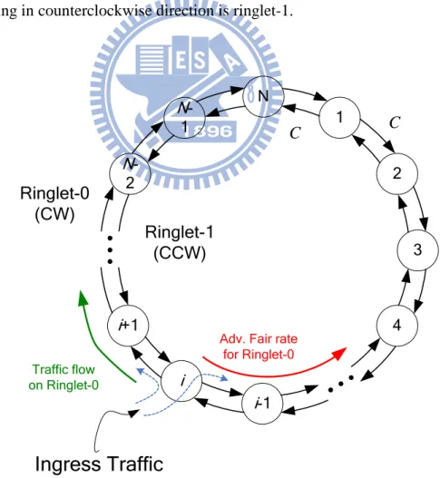
A dual-ring network contains two unidirectional ringlets and N nodes. As in Figure 2.1, the ringlet which is working in clockwise direction is ringlet-0. The ringlet which is working in counterclockwise direction is ringlet-1.

2 1 N 3 4 i-1 i+1 N -1 N -2 i Ringlet-1 (CCW) Ringlet-0 (CW)

Ingress Traffic

C C Traffic flow on Ringlet-0

Adv. Fair rate for Ringlet-0

(19)

The nodes are numbered in the clockwise manner from 1 to N. Each node is connected with two neighboring nodes. For simplicity, we assume that the distance between neighbor nodes is identical. And the propagation delay from node i to node

1 +

i is identical, too. For certain ringlet, we can differentiate the two neighbor nodes as an upstream neighbor and a downstream neighbor. For example, node i is directly connected with node i−1 and i+1. For clockwise directional ringlet-0, node i+1

is the downstream neighbor of node i . Each node is an ingress node as an originating LSR for MPLS-TP network and deals with the traffic from the access networks which are belong to it.

For simplicity, we also assume that the transmission capacity for each unidirectional link between neighbor nodes is equal to C identically. So at certain

time period t , the network has total 2tNC bandwidth resource to deal with the

traffic aggregated at each source node. We want to find out the optimal solution, which stands the minimum time period with QoS and fairness guarantees, to complete particular traffic demands.

2.2 Node Architecture

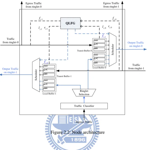
We propose the node architecture for MPLS-TP label switching router (LSR) is constructed by several components as Figure 2.2.

(20)

Traffic from ringlet-1 Traffic from ringlet-0 Ingress Traffic Output Traffic on ringlet-1 Output Traffic on ringlet-0 Traffic Classifier Scheduler Scheduler Local Buffer-0 B E A F E F Local Buffer-1 E F A F B E Transit Buffer-0 E B A F E F E F A F B E Transit Buffer-1 Egress Traffic from ringlet-0 Egress Traffic from ringlet-1 QLFG Ringlet Selection ,1 r f fr,0 ,1 v f ,0 v f ,1 y l ry,1 ly,0 y,0 r

Figure 2.2: Node architecture

The ingress local traffic classified at traffic classifier first. The classes of traffic is followed Diffserv, which used in MPLS-based network. The Diffserv model has been tested by IETF for traffic classification [27]. It is based on the aggregation of flows into a reduced number of classes. There is a 6-bit differentiated services code point (DSCP) field in the header of IP packets for packet classification purposes. Typically the traffic divided into three categories of services: expedited forwarding (EF), assured forwarding (AF) and best effort (BE) service. The EF service provides low delay and low loss performance which meets the requirements of reliable and real-time traffics. The AF service allows the operator to provide assurance of delivery as long as the traffic does not exceed some subscribed rate. Traffic that exceeds the

(21)

subscription rate faces a higher probability of being dropped if congestion occurs. AF service suits for the bandwidth required applications such as video over IP. BE service is the lowest priority class. Any traffic that does not meet the requirements of the other classes is placed in BE. Since the limited number of classes, the simplicity of scheduling algorithms and the limitation of the most complex mechanisms at ingress routers make Diffserv a scalable model.

After classification, the ingress local traffic will allocate to one of the two rings by ringlet selection. There are many kinds of algorithm to deal with the ringlet selection. The different strategy for ringlet selection would influence the traffic loading distribution on the two ringlets. Obliviously, it would also influence the network utilization. And to prevent loop storm in dual-ring network, each node makes the ring selection for local ingress traffic only. The transit traffic from two rings might be vanished if it is egress or dropped but never switched among the clockwise and counterclockwise rings. At the beginning of each flow, the local ingress node is in charge of making a path selection. The different generating orders of flow will introduce different path decisions since the traffic demand is dynamic and the dual-ring network load is changing time by time. Any time the local ingress packets arrived, ringlet selector must check the flow state table after packet classification and flow metering. If the flow state is existed in the table, the packet must follow the initial selection. Otherwise, the intra-flow out of order problem will be produced. For simplicity, we adopt round-robin strategy here.

Notice that, even though the reserving services subscribe a certain bandwidth, the ingress traffic loading is dynamic. So the bandwidth allocation for non-reserving services must be dynamic.

(22)

Then local ingress traffic split to different ring buffers. The transit traffic is also stored and classified in buffer for each ring. The buffers also collect the queue length

y

l and flow arrival rate r of each type of traffic from transit or local traffic (_y y:

t−EF , l−EF , t−AF , l−AF , t−BE , l−BE ,). Some of them might be aggregated as reservation traffic which will be defined in the next chapter. The information will take into consideration in fair rate generating.

The scheduler will transport the data from buffer to the downstream node with QoS guarantee for each traffic type by each ring. The local ingress traffic transmitting rate is constrained by the downstream node’s advertised fair rate. More details about the fairness control are show in section 2.3. And the advertised fair rate is produced by the Fuzzy Q-learning Fair rate Generator (QLFG). QLFG contains the fair rate control capability for BE traffic. QLFG takes l and _y r , which are collected from y

buffer queue and stand for the buffer queue length and arrival rate for certain y type traffic, into consideration. The y might be local/transit EF/AF/BE. It receives the advertised fair rate f from downstream node, computes a new fair rate by network _v

condition and its local traffic, advertises the new fair rate to its upstream node. More details about QLFG will show in the next chapter.

2.3 Fairness Model

In the transport network, if the nodes transmit data rate larger than the link capacity, an unfair bandwidth allocation problem occurs. The upstream nodes have more chance to transmit their data. The concept is to generate an advertised fair rate at

(23)

each node to regulate transit traffic flows. In order to define the meaning of fairness, an appropriate fairness model is indispensable. We choose a max-min fairness model for utilization optimization. The ring ingress aggregated with spatial reuse (RIAS) reference model was defined for RPR in the beginning.

The formal definition of RIAS [24] is described as follows: A matrix of rates R is

said to be RIAS fair if it is feasible and if for each flow(i,j) cannot be increased while

maintaining feasibility without decreasing Ri’,j’ for some flow(i’,j’) for which Ri,j’ ≤ Ri,j ,

(IA(i’) – IA(i)) at Bn(i,j) ≤ (IA(i’) – IA(i)) at Bn’(i,j), and IA(i’) ≤ IA(i) otherwise. The

definition ensures fair share between different IA flows and subflows of each IA flow. In RIAS model, the available bandwidth in current link will be fairly allocated among all ingress aggregated (IA) flows, where IA flow represents the aggregation of all flows originating from a specific ingress node. Furthermore, RIAS ensures maximal spatial reuse. That is, the unused bandwidth can be reallocated to other IA flows while maintaining fairness among the IA flows. Note that the RIAS model only takes single ring in consideration which is imperfect efficient for dual-ring networks. That’s why we need traffic engineering techniques to achieve network load balancing. If we do the ring selection appropriately, the traffic loading among two rings should be balanced. Then if we tune the transmitting rate for each flow satisfied RIAS model in each ring, we can say the dual-ring network is fair. Note that RIAS model assume each flow is greedy. Even though the final target rate for each IA which travel through the congestion link are fair, the rate tuning procedure should consider the finite bandwidth querying by each IA. Otherwise, the permanent oscillation would be severe which make slow convergence.

(24)

Chapter 3 Fuzzy Q-learning Fair Rate Generator

3.1 Fuzzy Q-learning Fair Rate Generator

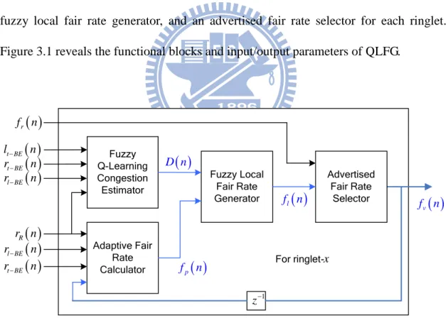
The Fuzzy Q-learning Fair Rate Generator (QLFG) contains four functional blocks: an adaptive fair rate calculator, a fuzzy Q-learning congestion estimator, a fuzzy local fair rate generator, and an advertised fair rate selector for each ringlet. Figure 3.1 reveals the functional blocks and input/output parameters of QLFG.

Fuzzy Q-Learning Congestion Estimator Fuzzy Local Fair Rate Generator

_{( )}

v f n

( )

D n

( )

r f n Adaptive Fair Rate Calculator fp

( )

n Advertised Fair Rate Selector

( )

t BE r₋ n

( )

l BE r₋ n

( )

R r n

( )

t BE r₋ n

( )

t BE l₋ n

( )

l f n

( )

l BE r₋ n 1 z− For ringlet-x

Figure 3.1: Functional blocks of QLFG

The fairness control scheme, which called fairRate, defined in IEEE 802.17 is implemented congestion control in each node. The downstream node generates an

(25)

advertised fair rate periodically to advertise its upstream node for regulating the added fairness-eligible traffic flow. We adopt the fair rate scheme and generate two fair rates individually for two ringlets. As the same time, the flows belong to different types traffic may select the two rings with different considerations to guarantee the quality of services. Since we have to guarantee the bandwidth of EF and AF type traffic, the only factor we can tune is BE type traffic transmission rate.

During the n th aging interval which is from time (n−1)T to nT, the QLFG

determines the advertise fair rate, denoted by f_v

( )

n . The fuzzy q-learning congestion

estimator will estimate the congestion degree D n of the local node according to the

( )

buffer queue length and flow arrival rate. Besides traditional fuzzy inference system, we add the Q-learning ability for it. The fuzzy rule base output of the congestion estimator become changeable by q-function and the reinforcement signal which is called rate difference. And then the congestion estimator transmits the congestion degree to the fuzzy local fair rate generator.

The adaptive fair rate generator collects the received fair rate which advertised from downstream nodes, the reservation bandwidth for EF and AF traffic, the flow arrival rate of transit BE traffic, and the flow arrival rate of local existing BE traffic. Then generating a provisional fair rate f_p

( )

n and transmit to the fuzzy local fair rate

generator.

The fuzzy local fair rate generator will generate a local fair rate f n , according l

( )

to provisional fair rate fp

( )

n and the congestion degree D n . Finally, the

( )

advertised fair rate selector will choose the received fair rate or the local fair rate as the advertised fair rate and transmit to upstream node by the opposite direction ringlet.

(26)

3.2 Fuzzy Q-learning Congestion Estimator

Considering for certain ringlet- x , the fuzzy congestion estimator is in charge of generating the congestion degree, denoted by D n , at the n -th aging interval for

( )

local fair rate generator. Since the larger flow arrival rate will increase the buffer queue length if serving rate non-changed, the congestion degree is determined not only by the

buffer queue length of transit BE type traffic at the n -th aging interval, denoted by

( )

t BE

l₋ n , but also by the flow arrival rate at the n -th aging interval, denoted by

( )

t BE

r₋ n .

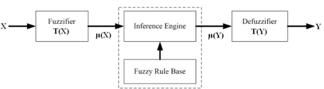
In our design, we adopted fuzzy logic control system to deal with the calculation. The typical structure of a fuzzy logic control system, shown in Fig. 3.2, comprises of four principal components: a fuzzifier, a fuzzy rule base, an inference engine, and a defuzzifier. The fuzzifier transforms crisp measured input variables X into suitable fuzzy linguistic terms. These fuzzy linguistic terms are specified by membership functions μ(X) and defined in a term set T(X). The fuzzy rule base stores the empirical knowledge, which is described by a collection of fuzzy control rules (e.g., IF-THEN rules) involving linguistic variables. These rules describe the relationship between the input variable X and the control action Y. The inference engine is the kernel of a FLC. It simulates human decision-making by performing an inference method to yield a desired control, which is described as fuzzy linguistic terms. These fuzzy linguistic terms are specified by membership functions μ(Y) and defined in a term set T(Y). The

(27)

defuzzifier is used to transform the inferred fuzzy control action to a non-fuzzy control action Y.

Figure 3.2: The basic structure of a fuzzy logic control system

Typically in traffic control area, we use the triangular function f x x a a ( ; ₀, ₀, ₁) and the trapezoidal function g x x x a a to define the membership functions for ( ; ₀, ,₁ ₀, ₁) terms in the term set. These two functions are given by

0 0 0 0 0 0 0 0 1 0 0 1 1 1, if , ( ; , , ) 1, if , 0, otherwise, x x x a x x a x x f x x a a x x x a a  − ₊ ₋ _{< ≤}    − =_ + < < +     (3.1) and 0 0 0 0 0 0 1 0 1 0 1 1 1 1 1 1 1, if , 1, if , ( ; , , , ) 1, if , 0, otherwise, x x x a x x a x x x g x x x a a x x x x x a a −  ₊ ₋ _{< ≤}    _{< ≤}   =  ₋  ₊ _{< < +}     (3.2)

(28)

where x in ₀ f( )⋅ is the center of the triangular function; x (₀ x ) in ₁ g( )⋅ is the left (right) edge of the trapezoidal function; a (₀ a ) is the left (right) width of the ₁

triangular or the trapezoidal function. The center, edge, or width of the triangular or trapezoidal membership function is set intuitively but based on the characteristics of the linguistic variables.

Term sets for the input are defined as T l

(

_{t BE}₋

( )

n

)

={Short (S), Long (L)}, and

( )

(

t BE

)

T r₋ n ={Low (L), Medium (M ), High (H)}. The Term set for the output

linguistic variables is defined as T D n

(

( )

)

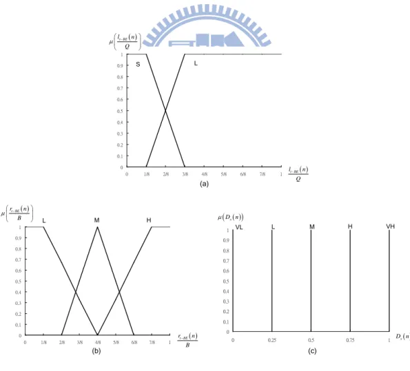
={ Very Low (VL), Low (L), Medium (M ), High (H), Very High (VH)}.

0 0.1 0.2 0.3 0.4 0.5 0.6 0.7 0.8 0.9 1 0 1/8 2/8 3/8 4/8 5/8 6/8 7/8 1 ( ) t BE l n Q µ −      ( ) t BE l n Q − S L (a) 0 0.1 0.2 0.3 0.4 0.5 0.6 0.7 0.8 0.9 1 0 1/8 2/8 3/8 4/8 5/8 6/8 7/8 1 ( ) t BE r n B µ −      ( ) t BE r n B − M L (b) H 0 0.1 0.2 0.3 0.4 0.5 0.6 0.7 0.8 0.9 1 0 0.25 0.5 0.75 1 ( ) (D nx ) µ ( ) x D n L (c) VL M H VH

Figure 3.3: The membership function of the term set (a) T l

(

_{t BE}₋

( )

n

)

(b) T r

(

_{t BE}₋

( )

n

)

(c) T D n

(

( )

)

(29)

Membership functions for terms of S, L, and H in T l

(

_{t BE}₋

( )

n

)

are defined as

( )

(

)

(

( )

; 0, 0.125 , 0, 0.25

)

, S lt BE n g lt BE n Q Q µ ₋ = ₋ (3.3)

( )

(

)

(

( )

; 0.35 , , 0.25 , 0 ,

)

L lt BE n g lt BE n Q Q Q µ ₋ = ₋ (3.4)

where Q is the size of transit BE queue. Membership functions for terms of L, M , and H in T r

(

_{t BE}₋

( )

n

)

are defined as

( )

(

)

(

( )

; 0, 0.125 , 0, 0.375

)

, L rt BE n g rt BE n B B µ ₋ = ₋ (3.5)

( )

(

)

(

( )

; 0.5 , 0.25 , 0.25

)

, M rt BE n f rt BE n B B B µ ₋ = ₋ (3.6)

( )

(

)

(

( )

; 0.875 , , 0.375 , 0 ,

)

H rt BE n g rt BE n B C B µ ₋ = ₋ (3.7)

where B n is the BE available bandwidth calculated as

( )

R

( )

B n = −C r n

. (3.8)

And r_R

( )

n represents the reservation bandwidth for EF/AF traffic,

( )

R t EF l EF t AF l AF

r n =r₋ n +r₋ n +r₋ n +r₋ n (3.9)

For the reason of simplicity in computation complexity of defuzzification, the corresponding membership functions of VL,L, M , H, and VH in T D n

(

( )

)

are defined as

( )

(

)

(

( )

; 0, 0, 0 ,

)

VL D n f D n µ = (3.10)

( )

(

)

(

( )

; 0.25, 0, 0 ,

)

L D n f D n µ = (3.11)

( )

(

)

(

( )

; 0.5, 0, 0 ,

)

M D n f D n µ = (3.12)

(30)

( )

(

)

(

( )

; 0.75, 0, 0 ,

)

H D n f D n µ = (3.13)

( )

(

)

(

( )

;1, 0, 0 .

)

VH D n f D n µ = (3.14)

Then we adopt Q-learning ability into the fuzzy inference system. Let

( )

(

( )

,

( )

)

x t BE t BE

X n = l₋ n r₋ n denote the vector of input linguistic variables, and S , _m

for m = 1, . . . , 6, denote the fuzzy linguistic terms of X n at n th interval. The

( )

fuzzy Q-learning rule for congestion estimator can then be designed as:

Rule m : if X n is

( )

S , then _m D with _k q_n

(

S_m,D , for 1 _k

)

≤ k ≤ 5,

(3.15) where D is the value of congestion degree with _k 0.25

(

k− and 1

)

q_n

(

S_m,D_k

)

is the Q-value for the state-action pair (S ,_m D ). The space of _k q_n

(

S_m,D is 30 since there _k

)

are 6 rules and 5 output terms. The Q-value can be viewed as the preferring value for each D under different input state. Note that, the value of _k q_n

(

S_m,D is learned by _k

)

the reinforcement signal at each episode. The intensity X n belongs to

( )

S , also _m

called the rule intensity, is obtained by

( )

(

( )

)

(

( )

)

,

m n α lt BE n β rt BE n

µ =µ ₋ ×µ ₋ (3.16)

where α ∈{S, L} and β ∈{L, M , H}. For each rule m , we choose the D _k

with maximum Q-value as the most suitable action for this input state. Let this selected action for rule m be am

( )

n . The global optimal action, denoted by a X n n

(

( )

,

)

,

can then be obtained by

( )

(

)

( )

6 1 6 1 , . m m m m m m n a n a X n n n µ µ = = = × =

∑

(3.17)

(31)

( )

(

,

)

a X n n is the output value of D n . Also, the Q-value for the state action is

( )

(

( )

)

(

)

( )

(

( )

)

( )

6 1 6 1 , , , . m n m m m m m m n q S a n Q X n a X n n n µ µ = = = × =

∑

(3.18)

Since the main idea of reinforcement learning to learn an optimal value such that the accumulation of benefit can be maximized in the future. Watkins and Dayan proposed a strong off-policy method to obtain the optimal Q-function. The value of Q-function, denoted by q_n

(

S_m,D_k

)

, updates recursively according to the rate

difference r n . Once the state-action pair has been determined, the rate difference _d

( )

d

r n can be obtained as the summation of the transit flow rate r_{t BE}₋

( )

n , the local add flow rate r_{l BE}₋

( )

n , and the negative available bandwidth −B n

( )

:

( )

,

d t BE l BE

r n =r₋ n +r₋ n −B n (3.19)

where B n

( )

= −C r_R

( )

n . Note that the fair rate assignment should minimize the oscillation effect. We find out that r n can reveal the convergence condition of the _d

( )

network flows. r n varies from _d

( )

−C to C. Every time the available bandwidth changes, the flows constrained by fair rate will oscillation for a certain period. Besides the flow rates from each nodes, the magnitude of rate difference r n decreases and _d

( )

converges to zero during the period. So we take the rate difference as reinforcement signal:

( )

(

( )

)

(

)

( )

_{( )}

₍

_{( )}

₎

( )

_{( )}

₍

_{( )}

₎

, if 0 , 1 , , , if 0 , 0 d d d d r n r n a X n n C r X n a X n n r n r n a X n n C  > ∧ <  =  − < ∧ >  . (3.20)

(32)

The idea is if the rate difference is positive, which means the summation of transit flow and local add flow rate exceed the available bandwidth, the congestion degree should become higher to overdose the local fair rate. Vice versa, if the rate difference is negative, which means the summation of transit flow and local add flow rate unfulfilled the available bandwidth, the congestion degree should become lower to release up the local fair rate. Then the value of q_n₊₁

(

S_m,D_k

)

can then be updated from q_n

(

S_m,D_k₋₁

)

or q_n

(

S_m,D_k₊₁

)

as

( )

(

)

(

( )

)

(

( )

)

1 , 0.25 , 0.25 , n m m n m m n m m q ₊ S a n + =q S a n + + × ∆η q S a n (3.21) if r n_d

( )

> ∧0 a_m

( )

n < , or 1

( )

(

)

(

( )

)

(

( )

)

1 , 0.25 , 0.25 , n m n m n m m q ₊ S a n − =q S a n − + × ∆η q S a n (3.22) if r n_d

( )

< ∧0 a_m

( )

n > , 0

where η∈

[ ]

0,1 is a learning rate and

( )

(

)

( )

{

(

( )

(

( )

)

( )

(

( )

)

(

)

(

)

(

( )

)

(

)

}

5 1 6 1 6 1 , , , , , 1 , 1 m n m m k k k k n k k k k k k n q S a n r X n a X n n n Q X n a X n n n q S a n n µ µ µ γ µ = = = = = ∆ = × − + × + × +

∑

.

γ is the discounted factor.

The procedure of fuzzy Q-learning algorithm is initialize q0

(

Sm,Dk

)

at first and

then by following steps: receive X n and find out

( )

am

( )

n → compute

( )

(

,

)

(33)

receive r X n a X n n

(

( )

,

(

( )

,

)

→ update q_n

(

S_m,D and back to the first step. _k

)

3.3 Adaptive Fair Rate Calculator

The adaptive fair rate calculator is designed to calculate a provisional fair rate

( )

p

f n and transmit it to the fuzzy local fair rate generator. The provisional fair rate

( )

p

f n can been seen as the base of the local fair rate f_{l x}_,

( )

n where is tuned by

fuzzy local fair rate generator according to congestion degree.

The concept of fairness is based on the RIAS model. We denote M n( ) as the equivalent number of IA transit flows traversing node i at n th aging interval. The

( ) M n is determined by  ( ) ( ) ( ) , ( 1) t BE l BE v r n r n M n f n − − + = −  (3.23)

where r_{l BE}₋ ( )n is the flow arrival rate of ingress BE traffic at the n -th aging interval,



(

)

1 1 ( 1) n v v i n k f i f n k = − + − − =

∑

and -

( )

1 ( ) n t BE t BE i n k r i r n k − = − + =

∑

 _{is the moving average of}

, ( 1)

v x

f n− and r_{t BE}₋

( )

n , which is the advertised fair rate generated at the (n−1)-th aging interval and the flow arrival rate of transit BE traffic at the n -th aging interval. Since the ring network might be large, the propagation delay would also be high. We must take the time-average to eliminate influence of the propagation delay.

So we can calculate a provisional fair rate of ringlet- x at the n -th aging interval, denoted by f n_p( ), by 1 ( ) min ( ), ( 1) ( ( ) ( ( ) ( ))) , ( ) p R v R l BE t BE f n C r n f n C r n r n r n M n − −   = _ − − + − − + _  

(34)

(3.24) where r n is the reservation bandwidth for EF/AF traffic at the n -th aging _R( )

interval.

3.4 Fuzzy Local Fair Rate Generator

The fuzzy local fair rate generator is designed to find a suitable value of local fair rate for BE-type traffic of certain ringlet- x . The function of fair rate is to limit the excess upstream nodes’ traffic. A congestion node generates an advertised fair rate. Then the upstream nodes receive the advertised fair rate via the opposing ringlet. We take the provisional fair rate, denoted by f n , and the congestion degree _p( ) generated from congestion estimator of ringlet- x at the n -th aging interval, denoted by D n , as fuzzy linguist input.

( )

0 0.1 0.2 0.3 0.4 0.5 0.6 0.7 0.8 0.9 1 0 0.1 0.2 0.3 0.4 0.5 0.6 0.7 0.8 0.9 1 ,( ) p x f n B µ    ,( ) p x f n B EL (a) PL SL SH PH EH

(35)

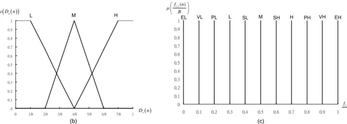
0 0.1 0.2 0.3 0.4 0.5 0.6 0.7 0.8 0.9 1 0 1/8 2/8 3/8 4/8 5/8 6/8 7/8 1 ( ) (D nx ) µ ( ) x D n M L (b) H 0 0.1 0.2 0.3 0.4 0.5 0.6 0.7 0.8 0.9 1 0 0.1 0.2 0.3 0.4 0.5 0.6 0.7 0.8 0.9 1 ,( ) l x f n B µ    ,( ) l x f n B L (c) VL M H VH EL PL SL SH PH EH

Figure 3.4: The membership function of the term set (a) T f

(

_{p x}_, ( )n

)

(b) T D n

(

_x

( )

)

(c) T f

(

_{l x}_, ( )n

)

The fuzzy term set of f_{p x}_, ( )n , denoted by T f

(

p x_, ( )n

)

, are Extremely Low

(EL), Pretty Low (PL), Slightly Low (SL), Slightly High (SH), Pretty High (PH), and Extremely High (EH ). The fuzzy term set of D n , denoted by x

( )

T D n

(

x

( )

)

,

are Low (L), Medium (M), and High (H). And the fuzzy term set of f_{l x}_, ( )n ,

denoted by T f

(

_{l x}_, ( )n

)

, are Extremely Low (EL), Very Low (VL), Pretty Low (PL), Low (L), Slightly Low (SL), Medium (M ), Slightly High (SH), High (H), Pretty High (PH), Very High (VH), and Extremely High (EH ).

Membership functions for terms of EL, PL, SL, SH , PH , and EH in

(

p x, ( )

)

T f n are defined as

(

, ( )

) (

, ( ); 0, 0, 0.3

)

, EL fp x n f fp x n B µ = (3.25)

(

, ( )

) (

, ( ); 0.2 , 0.2 , 0.2

)

, PL fp x n f fp x n B C B µ = (3.26)

(

, ( )

) (

, ( ); 0.4 , 0.2 , 0.2

)

, SL fp x n f fp x n B C B µ = (3.27)

(

, ( )

) (

, ( ); 0.6 , 0.2 , 0.2

)

, SH fp x n f fp x n B C B µ = (3.28)

(36)

(

, ( )

) (

, ( ); 0.8 , 0.2 , 0.2

)

, PH fp x n f fp x n B B B µ = (3.29)

(

, ( )

) (

, ( ); , 0.3 , 0 ,

)

EH fp x n f fp x n B B µ = (3.30)

where B n is the BE available bandwidth defined as eqn (3.8) in section 3.2.

( )

Membership functions for terms of L, M , and H in T D n

(

_x

( )

)

are defined as

( )

(

)

(

( )

; 0, 0.25, 0, 0.25 ,

)

L D nx g D nx µ = (3.31)

( )

(

)

(

( )

; 0.5, 0.25, 0.25 ,

)

M D nx f D nx µ = (3.32)

( )

(

)

(

( )

; 0.75,1, 0.25, 0 .

)

H D nx g D nx µ = (3.33)

For the reason of simplicity in computation complexity of defuzzification, the corresponding membership functions of T f

(

_{l x}_, ( )n

)

for terms of EL, VL, PL, L,

SL, M , SH, H, PH, VH, and EH are defined as

(

, ( )

) (

, ( ); 0, 0, 0 ,

)

EL fl x n f fl x n µ = (3.34)

(

, ( )

) (

, ( ); 0.1 , 0, 0 ,

)

VL fl x n f fl x n B µ = (3.35)

(

, ( )

) (

, ( ); 0.2 , 0, 0 ,

)

PL fl x n f fl x n B µ = (3.36)

(

, ( )

) (

, ( ); 0.3 , 0, 0 ,

)

L fl x n f fl x n B µ = (3.37)

(

, ( )

) (

, ( ); 0.4 , 0, 0 ,

)

SL fl x n f fl x n B µ = (3.38)

(

, ( )

) (

, ( ); 0.5 , 0, 0 ,

)

M fl x n f fl x n B µ = (3.39)

(

, ( )

) (

, ( ); 0.6 , 0, 0 ,

)

SH fl x n f fl x n B µ = (3.40)

(

, ( )

) (

, ( ); 0.7 , 0, 0 ,

)

H fl x n f fl x n B µ = (3.41)

(

, ( )

) (

, ( ); 0.8 , 0, 0 ,

)

PH fl x n f fl x n B µ = (3.42)

(37)

(

, ( )

) (

, ( ); 0.9 , 0, 0 ,

)

VH fl x n f fl x n B µ = (3.43)

(

, ( )

) (

, ( ); , 0, 0 ,

)

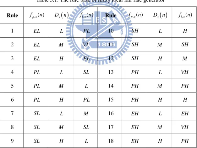
VH fl x n f fl x n B µ = (3.44)

There are 18 fuzzy rules for fuzzy local fair rate generator. As shown in Table 3.2, the order of significance of the input linguistic variables is fp x, ( )n then D n . The x

( )

fuzzy rule base is set by the concept that the value of f_{l x}_, ( )n mainly refers to f_{p x}_, ( )n

but slightly adjusted by D n so as to achieve lower convergence period and higher x

( )

the utilization.

Table 3.1: The rule base of fuzzy local fair rate generator

Rule fp x, ( )n D n x

( )

fl x, ( )n Rule fp x, ( )n D n x

( )

fl x, ( )n 1 EL L PL 10 SH L H 2 EL M VL 11 SH M SH 3 EL H EL 12 SH H M 4 PL L SL 13 PH L VH 5 PL M L 14 PH M PH 6 PL H PL 15 PH H H 7 SL L M 16 EH L EH 8 SL M SL 17 EH M VH 9 SL H L 18 EH H PH

Then the defuzzifier uses the max-min method for the inference engine to generate a crisp-values local fair rate because it is suitable for real-time operation. To

(38)

explain the max-min inference method, we take rule 7 and rule 12, which have the same control action “ f_{l x}_, ( )n is M,” as an example. Applying the min operator, we obtain the membership function values of the control action “ f_{l x}_, ( )n is M ” of rule 7 and rule 12, denoted by m n and 7

( )

m12

( )

n respectively, by m n7

( )

=min

(

)

(

( )

)

{

µSL fp x, ( ) ,n µL D nx

}

and m12

( )

n =min

{

µSH

(

fp x, ( ) ,n

)

µH

(

D nx

( )

)

}

.

Subsequently, applying the max operator yields the overall membership function value of the control action “ f_{l x}_, ( )n is M ” denoted by w_M

( )

n , by

( )

max

{

7

( )

, 12

( )

}

M

w n = m n m n . And as so as for EL, VL, PL, L, SL, SH, H,

PH , VH and EH, we can obtain all the output index. Finally, the fuzzy inference results are to be defuzzified to become usable values. By adopting the center of area defuzzification method, a crisp value of the local fair rate of ringlet- x at the n -th aging interval, denoted by fl x_, ( )n , can be obtained by

( )

, 0.1 0.2 0.9 ( ) VL PL H EH l x EL VL PL VH EH w n w n w n w n f n w n w n w n w n w n ⋅ + ⋅ + + ⋅ + = + + + +   . (3.45)

3.5 Advertised Fair Rate Selector

Finally the advertised fair rate selector observes the incoming transit BE traffic ( )

t BE

r₋ n , compares it with the minimum of the local fair rate f_{l x}_, ( )n and the received advertised fair rate from the other ringlet f_{r x}_, ( )n for ringlet- x . The main reason of using minimum operation is to be a little more conservative in order not to incur

(39)

overuse of a link too often. If r_{t BE}₋ ( )n is bigger than or equal to the minimum of

, ( )

l x

f n and f_{r x}_, ( )n , the link is considered as overused. So, fair rate scheme will

decrease the rates of IA flows, and choose the minimum of f_{l x}_, ( )n and f_{r x}_, ( )n as

the advertised fair rate f_{v x}_, ( )n . If r_{t BE}₋ ( )n is smaller than or equal to the minimum of f_{l x}_, ( )n and f_{r x}_, ( )n , the link is considered as not sufficiently used. So, FQFRG

will increase the rates of IA flows, and choose the maximum of f_{l x}_, ( )n and f_{r x}_, ( )n

as the advertised fair rate f_{v x}_, ( )n . The function is described as below:

If r_{t BE}₋ ( )n ≥ min ( f_{r x}_, ( )n , f_{l x}_, ( )n ), f_{v x}_, ( )n = min ( f_{r x}_, ( )n , f_{l x}_, ( )n ) ;

If r_{t BE}₋ ( )n < min ( f_{r x}_, ( )n , f_{l x}_, ( )n ), f_{v x}_, ( )n = max ( f_{r x}_, ( )n , f_{l x}_, ( )n ).

(3.46) However, we can simplify (3.46) as:

If f_{l x}_, ( )n > f_{r x}_, ( )n > r_{t BE x}_- _, ( )n , f_{v x}_, ( )n = f_{l x}_, ( )n ;

(40)

Chapter 4 Simulation Results and Discussions

4.1 Simulation Environment

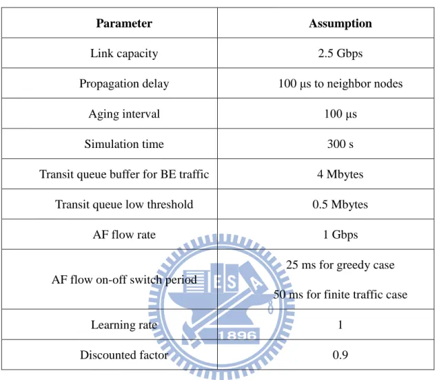
In the simulations, we compare the performance of QLFG with DBA and FLAG. The setting for the environment include 2.5Gbps link capacity, 100us propagation delay between nodes, 4Mbytes transit queue buffer for BE traffic, and 100us aging interval. The value of the transit queue high threshold is 1 Mbytes and the value of the transit queue low threshold is 0.5Mbytes. Simulation results are recoded per aging interval. For simplicity, we assume that no EF flow and only one AF traffic flow pass through each node and the rate is has 1Gbps. The learning rate η and discounted factor γ for fuzzy Q-learning congestion estimator is 1 and 0.9, respectively. The initial value of Q-function is based on the rule base of fuzzy congestion detector in FLAG [26]. We focus on the BE traffic flow rate variation of each node in the first period before it stable. All of the simulation parameters are shown as Table 4.1. The convergence time is obtained if the rate oscillation is in the range of 1% variation to its ideal fair rate.

(41)

Table 4.1: The simulation parameters

Parameter Assumption

Link capacity 2.5 Gbps

Propagation delay 100 μs to neighbor nodes

Aging interval 100 μs

Simulation time 300 s

Transit queue buffer for BE traffic 4 Mbytes

Transit queue low threshold 0.5 Mbytes

AF flow rate 1 Gbps

AF flow on-off switch period

25 ms for greedy case 50 ms for finite traffic case

Learning rate 1

Discounted factor 0.9

Followings are scenarios set to examine the fairness algorithms’ performance. We adopt the large parking lot scenario with greedy traffic flows and various finite traffic flows to observe the property of bandwidth fair share on congestion link. We will compare three figures for each scenario, which are flow throughput, congestion detection signals, and congestion node output rate.

(42)

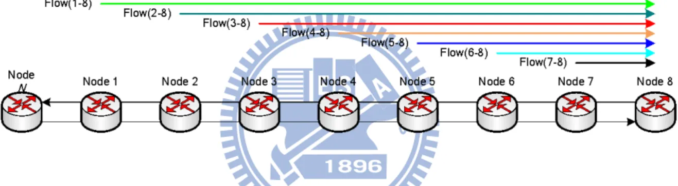
4.2 Large Parking Lot Scenario with Greedy Traffic Flows

Fig. 4.1 shows a large parking lot scenario where there are eight stations with seven greedy traffic flows. Node 1~7 all has a traffic flow to node 8, and the demand bandwidth are equal to the link capacity 2.5Gbps. There is one on/off AF traffic flow pass through each node. The rate of AF flow is 1Gbps when it switch on. And the switch period is 25ms.

Figure 4.1: Large parking lot scenario with greedy traffic flows.

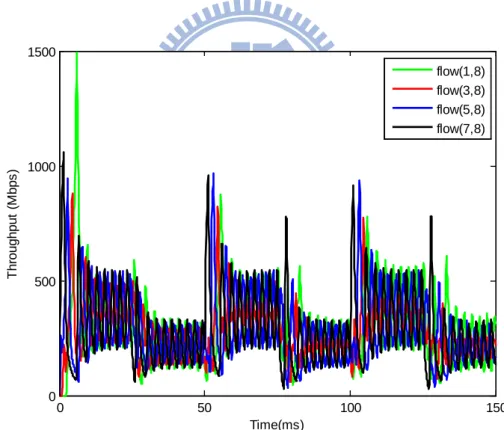
Figs 4.2(a), 4.2(b), 4.2(c) present the throughput of flow(1-8), flow(3-8), flow(5-8), and flow(7-8) at node 7 by DBA, FLAG, and QLFG, respectively. First we can see that the QLFG and the FLAG take less than 20ms to stabilize the traffic flows at the first 25ms. It can also be seen the flows are getting the same bandwidth about 357.1Mbps and it guarantee the fairness property. Even though the QLFG take a little longer time to stabilize the traffic flows than FLAG, the situation can be seen as an initial state. Unfortunately, DBA can not stabilize the traffic flows in 25ms. Then at 25ms, the AF flow starts transmitting with 1Gbps bandwidth. The available bandwidth for BE traffic flows decrease to 1.5Gbps. DBA still oscillate now and for all. The

(43)

reason of DBA oscillation is the propagation delay from node 7 to node 1 is large. It can be seen that the QLFG and the FLAG take 10.7ms and 18.8ms to stabilize the traffic flows at the 25ms to 50ms. It can also be seen the flows are getting the same bandwidth about 214.3Mbps and it still guarantee the fairness property. Then at 50ms, the AF flow terminates and the available bandwidth for BE traffic flows increase back to 2.5Gbps. It can be seen that the QLFG and the FLAG take 7ms and 10.6ms to stabilize the traffic flows at the 50ms to 75ms. The better saturation performance of QLFG is cause by the fuzzy Q-learning ability and taking the rate difference into account. 0 50 100 150 0 500 1000 1500 Time(ms) T hr oughput ( M bps ) flow(1,8) flow(3,8) flow(5,8) flow(7,8)

(44)

0 50 100 150 0 200 400 600 800 1000 1200 Time(ms) T hr oughput ( M bps ) flow(1,8) flow(3,8) flow(5,8) flow(7,8)

Figure 4.2 (b): Throughput of FLAG.

0 50 100 150 0 200 400 600 800 1000 1200 Time(ms) T hr oughput ( M bps ) flow(1,8) flow(3,8) flow(5,8) flow(7,8) Figure 4.2 (c): Throughput of QLFG.

(45)

We can see the difference between QLFG and FLAG clearly by Figs 4.3. Figs 4.3 (a), 4.2(b), 4.2(c) reveals the congestion detection on node 7 by DBA, FLAG, and QLFG, respectively. Focus on the AF flow switching time per 25ms. By taking the rate difference into account, the fuzzy Q-learning ability makes the congestion degree much sensitive. We can see the congestion degree increase quicker than FLAG at 50ms in QLFG. And it so does for the available bandwidth increasing at 500ms. Since the congestion degree becomes sensitive in QLFG, the advertised fair rate from node7 can make the network flows stable more quickly.

0 50 100 150 -1 -0.8 -0.6 -0.4 -0.2 0 0.2 0.4 0.6 0.8 1 Time(ms)

transit BE queue length / size rate diff. / capacity

transit BE arrival rate / capacity congestion degree

(46)

0 50 100 150 -1 -0.8 -0.6 -0.4 -0.2 0 0.2 0.4 0.6 0.8 1 Time(ms)

Figure 4.3 (b): Congestion detection on Node 7 by FLAG.

0 50 100 150 -1 -0.8 -0.6 -0.4 -0.2 0 0.2 0.4 0.6 0.8 1 Time(ms)

(47)

Figs 4.3(a), 4.3(b), 4.3(c) reveal the output rate of transit queue, local added queue, and advertised fair rate with BE available bandwidth switching at node 7 by DBA, FLAG, and QLFG, respectively. We can see the advertised fair rate by QLFG has less oscillation. The transit rate and local add rate is changing smoothly and properly because of the fuzzy Q-learning ability.

0 50 100 150 0 500 1000 1500 2000 2500 Time(ms) R at e ( M bps ) BE available bandwidth transit BE arrival rate local BE add rate adv. fair rate

(48)

Figure 4.4 (b): Node 7 Output by FLAG.

(49)

4.3 Large Parking Lot Scenario with Various Finite Traffic

Flows

Fig. 4.5 shows a large parking lot scenario where there are eight stations with seven non-greedy traffic flows. Node 1~7 all has a traffic flow to node 8. Assume that flow(1-8) and flow(2-8) require 650Mbps, flow(3-8) and flow(4-8) require 400Mbps, flow(5-8) and flow(6-8) require 200Mbps, and flow(7-8) requires 100Mbps. There is one on/off AF traffic flow pass through each node. The rate of AF flow is 1Gbps when it switch on. And the switch period is 50ms.

Figure 4.5: Large parking lot scenario with various finite traffic flows.

Figs 4.6(a), 4.6(b), 4.6(c) present the throughput of flow(1-8), flow(3-8), flow(5-8), and flow(7-8) at node 7 by DBA, FLAG, and QLFG, respectively. First we can see that the QLFG and the FLAG take about 21ms to stabilize the traffic flows at the first 50ms. Even though the QLFG take a little long time to stabilize the traffic flows than FLAG, the situation can be seen as an initial state as in the previous greedy

(50)

case. Unfortunately, DBA can not stabilize the traffic flows in 50ms. Then at 50ms, the AF flow starts transmitting with 1Gbps bandwidth. The available bandwidth for BE traffic flows decrease to 1.5Gbps. DBA still oscillate now and for all. The reason of DBA oscillation is the propagation delay from node 7 to node 1 is large. It can be seen that the QLFG and the FLAG take about 43ms to stabilize the traffic flows at the 50ms to 100ms. Then at 100ms, the AF flow terminates and the available bandwidth for BE traffic flows increase back to 2.5Gbps. It can be seen that the QLFG and the FLAG take 6.6ms and 10.9ms to stabilize the traffic flows at the 100ms to 150ms. Moreover, the flows can not converge well by FALG in 150ms to 200ms. QLFG takes 15.6ms to stabilize the flows except flow(1-8) and flow(2-8) with about 13Mbps variation. The better saturation performance of QLFG is cause by the fuzzy Q-learning ability and taking the rate difference into account.

It can also be seen the flows are getting the bandwidth by their demands and it guarantee the max-min fairness property. Flow(7-8) is smoothly transmitting at 100Mbps for all scheme. However, flow(5-8) with 200Mbps demands can not saturated in DBA. When AF flow switch on, the oscillation become more severe. The phenomenon is also occurred in FLAG. Even though flow(5-8) got sufficient bandwidth when AF flow switch off, it can not keep in 200Mbps stable when AF flow switch on. In QLGR, the rate of flow(5-8) vitiate after the AF switch time only. And the convergence rate is correct. So does for the other flows. The advertised fair rate correctly constraint those overdose flows with 400Mbps or 650Mbps demands at 250Mbps rate.

(51)

0 50 100 150 200 250 300 350 400 0 200 400 600 800 1000 1200 Time(ms) T hr oughput ( M bps ) flow(1,8) flow(3,8) flow(5,8) flow(7,8)

Figure 4.6 (a): Throughput of DBA.

0 50 100 150 200 250 300 350 400 0 100 200 300 400 500 600 700 Time(ms) T hr oughput ( M bps ) flow(1,8) flow(3,8) flow(5,8) flow(7,8)

使用Fuzzy Q-learning達成具公平性動態頻寬分配的MPLS-TP環

國

立

交

通

大

學

電機學院通訊與網路科技產業研發碩士班

碩

士

論

文