國際收支失衡與資本適足率最適調整之探討—以歐元區為例 - 政大學術集成

全文

(1)國立政治大學國際經營與貿易學系碩士論文 Department of International Business National Chengchi University Master Thesis. 治 Trade Imbalance 政 and Adjustment 大 of Capital 立. ‧ 國. 學. Requirement in Euro Area. 國際收支失衡與資本適足率最適調整之探討—. ‧. 以歐元區為例. n. er. io. sit. y. Nat. al. Ch. engchi. i Un. v. 指導教授: 胡聯國博士 Advisor: Hu, Len-Kuo, Ph.D.. 研究生:蕭筑方 Hsiao, Chu-Fang. 中華民國 101 年 6 月 June, 2012.

(2) 謝誌研究所的時光過得好快，至今還記得當初剛揮別大學、迎接研究所來臨時，那感傷卻又參雜著興奮的心情。這段時光雖然短暫而緊湊，然而我卻吸收成長了許多，也接觸學習到更多更廣闊的領域。很感謝指導教授胡聯國教授的教導，不論是在課堂中或是研究方面，都能感受到教授廣博且精深的學問，每次教授的談話也總是讓我有所感觸並且受益良多。更特別感謝教授在奔波忙碌之餘，儘管是最忙碌的時刻，仍特地撥出時間耐心指導，更不忘關心詢問近況。每每在我感到山窮水盡之際，教授從旁的啟發與教導，引領我度過了層層關卡。. 立. 政治大. 此外，也十分感謝口試委員龔尚智教授與林柏生教授的指導，並且給予論文. ‧ 國. 學. 關鍵精闢的建議，使我瞭解更多研究上的不足與使論文更臻完善的努力方向。. ‧. 還要謝謝一路陪伴我走來的老友們與研究所的好友們，謝謝你們所有無形與. sit. y. Nat. 有形的鼓勵，也難忘你們增添在我生活中的許多歡笑與回憶。謝謝我認真又有毅. io. al. er. 力的研究夥伴—均亭，不論時間如何流逝，將不會忘記那些我們共同打拚作戰的. n. 日子，妳的打氣與笑語常是我繼續往前突破難關的動力，也是我在研究期間珍貴的歡樂來源。. Ch. engchi. i Un. v. 最後，感謝我親愛的家人，這一路的成長，因為有您們在我身旁鼓勵，每當我面臨難題時，也總是不厭其煩地聆聽與開導，並且相信與全力支持我的每一個抉擇，使我能無後顧之憂、更加有勇氣地迎接所有前來的挑戰。. 蕭筑方謹誌于政大.

(3) 摘要目前歐盟訂立的歐盟資本要求規範(Capital Requirements Directive)是為加強歐元區內的金融機構之間的風險管理並參考新巴塞爾資本協定(New Basel Capital Accord)所建構而成的風險管理規範。本文之理論基礎是以 Holmström and Tirole (2011)流動性衝擊之模型與 Hu (2012)資本適足率之模型為基底，從國際貿易的觀點繼續延伸，探討當考慮國際收支帳之後，資本適足率應當如何加以調整，並且探討目前歐元區全面遵循一致的資本要求規範之現象是否合適。由於歐元區各國的貿易失衡問題也是造成當前歐洲債務危機的主要因素之一，因此，本文也. 政治大. 將觀察貿易失衡與調整資本適足率之間的關係。最後，本文以歐元區 17 國最近. 立. 6 年的經濟統計資料套用理論模型並經過實證之後發現，歐元區各國對於資本適. ‧ 國. 學. 足率調整之方向並非一致，此外，由於各國在每個時期的經濟表現也不盡相同，. ‧. 因此，歐盟應更多加思考歐元區各國不同的資本調整之特性與總體經濟表現來修訂資本要求規範。. n. al. Ch. engchi. i. er. io. sit. y. Nat 關鍵字：資本適足率、貿易失衡、歐洲貨幣聯盟. i Un. v.

(4) ABSTRACT The European Union constructs a comprehensive and risk-sensitive framework, Capital Requirements Directive (CRD), to enhance risk management among financial institutions. This paper analyzes whether the rules of capital requirement ratios should be uniform for all the countries in Euro area by establishing a model of liquidity shock and capital requirement from the sight of balance of payments. This paper will also observe the relationships between current account imbalances and the adjustment. 政治大 of the reasons that cause nowadays 立 European debt crisis. The results of the model. of capital requirement, because international trade imbalances also account for parts. ‧ 國. 學. show that uniform policy for capital requirement is not appropriate for all the EU-17. The adjustment of capital requirement should be considered for the various. ‧. macroeconomic environments in different countries and in different times.. sit. y. Nat. n. al. er. io. Keywords: Capital regulation, trade imbalance, European monetary union. Ch. engchi. ii. i Un. v.

(5) CONTENTS 摘要. ………………………………………………………………………….....i. ABSTRACT ...................................................................................................................ii 1 Introduction ................................................................................................................. 1 2 Literature Review ........................................................................................................ 5 2.1 Public Debt............................................................................................... 5 2.2 Capital Requirement ................................................................................ 5 2.3 Trade Imbalance ....................................................................................... 7 3 The Model ................................................................................................................. 10 3.1 Background ............................................................................................ 10 3.2 Liquidity Shock ...................................................................................... 12 3.3 Balance of Payment ............................................................................... 15. 政治大 4 The Empirical Model ................................................................................................ 19 立 4.1 Data ........................................................................................................ 19 ‧. ‧ 國. 學. 4.2 Statistics of Economics Environment in EU-17 .................................... 19 4.2.1 Current Account .......................................................................... 19 4.2.2 Growth Rate of Output................................................................ 20 4.2.3 Debt to GDP Ratio ...................................................................... 21 4.3 Comparison of the Interest Rate Sensitivity of Output between EU-17 25. y. Nat. sit. n. al. er. io. 4.4 The Method of Regression ..................................................................... 29 4.4.1 Unit Root Test ............................................................................. 29 4.5 Variables, Explanations, and Results of Regression .............................. 31 4.5.1 Variables ...................................................................................... 31 4.5.2 Results and Explanation .............................................................. 32 4.6 Estimation and Policy Suggestion ......................................................... 33 5 Conclusion ................................................................................................................ 37 Appendix A. ................................................................................................................. 38 Appendix B. ................................................................................................................. 48. Ch. engchi. i Un. v. Reference ..................................................................................................................... 49. iii.

(6) LIST OF FIGURES Table 1. The Classification of the Interest Rate Sensitivity of Output in EU-17 ......... 26 Table 2. Panel Unit Root Tests on the Original Data ................................................... 30 Table 3. Panel Unit Root Tests on the Variables with First Difference ........................ 30 Table 4. The Result of Panel Data Regression ............................................................. 32 Table 5. Suggestion of Policies for Capital Requirement in 2011 Q4 ......................... 36 Table 6. The Descriptions of Data ................................................................................ 38 Table 7. The Descriptions of Interest Rates (unit: percentage) .................................... 39 Table 8. The Results of Simple Regressions ................................................................ 40 Table 9. Values of the Interest Rate Sensitivity of Output (Unit: Index) ..................... 41 Table 10. Government Consolidated Gross Debt ......................................................... 42 Table 11. Trade Openness ............................................................................................ 43 Table 12. Explainable Variables in EU-17 ................................................................... 44 Table 13. Explainable Variables in EU-17 (continued) ................................................ 45 Table 14. Explainable Variables in EU-17 (continued) ................................................ 46 Table 15. Explainable Variables in EU-17 (continued) ................................................ 47. 立. 政治大. ‧ 國. 學. LIST OF TABLES. ‧. Fig 1. Current Account to GDP Ratios in EU-17 from 2005 Q1 to 2011 Q4 (Units: %) .......................................................................................................................... 22 Fig 2. GDP Growth Rates in EU-17 from 2005 Q1 to 2011 Q4 (Units: %) ................ 23 Fig 3: Debt to GDP Ratios in EU-17 from 2005 Q1 to 2011 Q4 (Units: %) ............... 24 Fig 4. The Interest Rate Sensitivity of Output in EU-17 from 2005 Q2 to 2011 Q3 ... 27 Fig 5. The Interest Rate Sensitivity of Output in EU-17 from 2005 Q2 to 2011 Q3 (continued) ....................................................................................................... 28 Fig 6. Estimation of the Interest Rate Sensitivity of Output, Growth Rate (%), and Current Account to GDP Ratio (%) in EU-17 in 2011 Q4 ............................... 35. n. er. io. sit. y. Nat. al. Ch. engchi. iv. i Un. v.

(7) 1 Introduction The European sovereign debt crisis represents a huge financial crisis in which some countries in the Euro area are unable to refinance their government debt independently or without the assistance of other countries. In the end of 2009, investors have started to worry about the Euro debt situations due to the rising government debt levels internationally and some downgrading of government debt in some European states. On 9 May 2010, the leading Europe’s finance ministers approved a rescue package worthy. 政治大 promote the financial stability 立across Europe. In October and February 2012, the of 750 billion euro dollars and created the European Financial Stability Facility to 1. ‧ 國. 學. Eurozone leaders agreed on more measures, including requiring European banks to achieve 9% capitalization, and created a European Fiscal Compact to introduce balanced. ‧. budget amendment from those participating countries.. Nat. sit. y. In order to construct a comprehensive and risk-sensitive framework and to enhance. n. al. er. io. risk management among financial institutions, European Commission has established. i Un. v. EU rules, Capital Requirements Directive (CRD), on capital requirements for credit. Ch. engchi. institutions and investment firms. The original framework of CRD was initially published in June 2004.2 The directives have kept amended and expanding from legislation in force, CRD I, CRD II and CRD III packages, to the newest proposals, CRD IV packages. The Capital Requirements Directive introduces a supervisory framework which is revised by Basel II rules on capital measurement and capital standards. The Basel. 1. "EU ministers offer 750bn-euro plan to support currency". BBC News. 10 May 2010. Retrieved 11 May 2010. 2 The detailed rules of Capital Requirements Directive are on the European Commission website, available in http://ec.europa.eu/internal_market/bank/regcapital/index_en.htm. 1.

(8) Accord, established in 1988 by Basel Committee on Banking Supervision, requires higher capital ratios to ensure the soundness and stability of international banking system. Basel II is composed of the concept of three pillars. Pillar I sets out the minimum capital requirements on firms. Pillar II requires firms and supervisors to observe whether there are risks which are not covered in Pillar I and increase additional capital if so. Third pillar requires firms to disclosure certain details of their risks, capital and risk management in order to complement the supervisory review process. After the financial crisis over 2008 and 2009, Basel III proposals improve deficiencies in Basel II to strengthen the regulatory regime. On 20 July 2011, the. 治政大 which referred to the European Commission also adopted a new CRD IV package, 立. reform in Basel III, in order to enhance more complete regulation on the banking sector.. ‧ 國. 學. This new legislative package is a key instrument to introduce the new European. ‧. supervisory structure.3. sit. y. Nat. To deliberate the causes of the European sovereign debt crisis, there are many. io. al. er. complex factors involved. Among those factors, international trade imbalances account for one of the reasons that caused today’s European debt crisis. If a country imports. n. iv n C more than exports, it runs a currenth account deficit iand e n g c h Uis a net importer of capital. This means that it will decrease its savings or borrow money to buy those imports. Conversely, a country with trade surplus is a net exporter of capital and its savings will increase, and it can lend money to other countries. In Eurozone, richer countries whose currencies are devalued keep surpluses in their current accounts, and poorer countries whose currencies are overvalued keep deficits in their current accounts. Countries with deficits in the current accounts will keep. 3. The explanations of CRD are from the website of UK Financial Services Authority, available in http://www.fsa.gov.uk/about/what/international/basel. 2.

(9) accumulating increasing debt or foreign ownership of domestic assets. During 1999-2007, Germany had a better performance of public debt and fiscal deficit relative to GDP than other Eurozone members. Estonia, Portugal, Greece, Ireland, Italy and Spain had worse balance of payments deficits which are considered to be the most vulnerable countries by the perspective on current account deficits, whereas Germany had an increased trade surplus as a percentage of GDP after 1999.4 Greece’s trading position has improved during 2011 to 2012. The percentage of imports has dropped 20.9% and the percentage of exports has grown 16.9%. Hence, the percentage of trade deficits is reduced by 42.8%.5. 治政大 can be reduced Although trade imbalances between different countries 立. automatically by the appreciation or devaluation of currencies, this mechanism is not. ‧ 國. 學. suitable in the countries within Euro area due to the fact that the countries within Euro. ‧. area all hold the same currency. The only solution to increase a country’s saving is to. sit. y. Nat. reduce budget deficits and change consumption and saving habits. For example,. io. al. er. countries with large trade deficits, like Greece, are suggested to consume or import less and encourage their exporting industries. While countries with large trade surpluses, like. n. iv n C Germany, Austria and the Netherlands, h eshould h i U more domestic goods and n g cconsume. services and increase wages to support domestic consumption. In May 2012, Wolfgang, German finance minister, has expressed the government will help decreasing current account imbalances within Eurozone by increasing the wages in Germany. This paper aims to analyze whether the rules of capital ratios should be identical for all the countries in Euro area. This study covers four steps. First, establish a model with. 4. Martin Wolf (6 December 2011). "Merkozy failed to save the eurozone". The Financial Times. Retrieved 9 December 2011. 5 “Commercial Transactions of Greece: March 2012 (estimations)". Hellenic Statistical Authority. statistics.gr. 29 May 2012. p. 10. Retrieved 6 June 2012. 3.

(10) liquidity shock from the sight of balance of payments to consider the appropriate capital requirement ratios. Second, put the recent data in 17 countries in the European Monetary Union into the established model. Third, consider some variables and run a panel data between EU-17 from 2005Q2 to 2011Q3. Finally, estimate how to adjust the appropriate capital requirement in the realistic economy environments in the different countries.. 立. 政治大. ‧. ‧ 國. 學. n. er. io. sit. y. Nat. al. Ch. engchi. 4. i Un. v.

(11) 2 Literature Review 2.1 Public Debt Governments often issue government debt to make the fiscal policy. Although appropriate debt could help the economy to go well, the amount of debt is not always good for the economy. Debt will have a great positive or negative impact on the social economy depending on its amount in different countries. Checherita, Cristina, and Rother (2010) found that debt levels of around 70-80% of GDP start to have a negative. 政治大. effect on per-capita GDP growth, and beyond the turning point, about 90-100% of GDP,. 立. the debt will have a deleterious impact on growth in 12 Euro area countries over a period. ‧ 國. 學. of about 40 years since 1970. Cecchetti, Mohanty, and Zampolli (2011) also support that debt is a burden on growth beyond a certain level, and governments should keep debt. ‧. below the estimated thresholds of government debt, around 85% of GDP.. sit. y. Nat. er. io. 2.2 Capital Requirement. al. n. iv n C U the regulators can screen banks Morrison and White (2005) sethup eanmodel g c hin iwhich to decide whether giving licenses and imposing capital requirement on them. In this model, it is suggested that countries with worse regulator reputation should have a tighter capital regulation, and countries with better reputation should have a looser capital regulation. From the banks’ side, if a bank’s investment is more transparent, then its capital requirements can be looser. In Blundell- Wignall and Atkinson (2010)’s review for the history of Basel Accords, Basel I developed in 1988 and came into effect in 1992. The aim of Basel I was to require enough capital in banks in avoid of causing systemic problems and to avoid 5.

(12) competitiveness internationally. Because under Basel I banks accumulated capital more than regulatory minimum requirements which had no constraining impact on the risk taking of banks, a new accord, Basel II, was released in 2004. In the Basel system the capital regulations are pro-cyclicality. It’s mainly because that it’s easy to underestimate risks in good times but overestimate risks in bad times. However, there is still room for revises for Basel II. Kashyap and Stein (2004) state that Basel II with only a single time-invariant risk curve is suboptimal. It’s because from the social planner’s view, not only bank defaults should be considered, but also the efficiency of bank lending should be. Hence, it’s more complete to have a family of. 治政大 That is, the policy for point-in-time risk curves in different macroeconomic conditions. 立 capital is scarce relative to lending opportunities.. 學. ‧ 國. the capital requirement should tolerate higher probabilities of default when the bank. ‧. In response to the problems of capital regulation found by the late-2000s financial. sit. y. Nat. crisis, the Basel Committee revised Basel Accords and developed Basel III in 2010.. io. er. Blundell- Wignall and Atkinson (2010) review that Basel III has reformed the quality,. al. consistency and transparency of the capital base, enhanced risk coverage, proposed a. n. iv n C “backstop” leverage ratio, and dealthwith pro-cyclicality e n g c h i U through dynamic provisioning based on expected losses. Slovik and Cournede (2011) estimate medium-term impact of implementing Basel III on GDP growth in the 3 main OECD economies is in the range of -0.05 to -0.15 percentage point per annum. This estimation is under the assumption that there is no response from monetary policy. If considering the effect from monetary policy, a macroeconomic impact of Basel III on the annual GDP growth of -0.05 to -0.15 percentage points could be offset by an average reduction in the monetary policy rates of about 30 to 80 basis points. 6.

(13) 2.3 Trade Imbalance In Krugman’s (1979) model of balance-of-payments crises, if a country keeps issuing money or making use of its reserves to finance the fiscal deficit, to some extent the reserves will be exhausted. At that time, it will lead to a sudden collapse of fixed exchange-rate regime, called the balance-of-payments crises. Currency crises will also accompany the balance-of-payments crises when the price level begins rising and the currency gradually depreciates due to the increasing nominal money supply. Kaminsky and Reinhart (1999) organize that most of the former literature. 政治大. emphasized on the inconsistency between fiscal and monetary policies and the. 立. exchange-rate commitment, or on the self-fulfilling expectations and herding behavior in. ‧ 國. 學. international capital markets. However, seldom literature studied the interaction between. ‧. banking and currency problems. In their studies for a number of industrial and developing countries, they find that after the liberalization of financial markets across. y. Nat. er. io. sit. many countries, banking and currency crises become closely linked. Problems in the banking sector often come before a currency crisis. The currency crisis deepens the. n. al. Ch. i Un. v. banking crisis and causes a vicious spiral. Although banking crises often precede. engchi. balance-of-payments crises, they are not the immediate cause of currency crises. Both of them are preceded by recessions, a worsening of the terms of trade, an overvalued exchange rate, and the rising cost of credit. The crises typically come after a series of weak and deteriorating economic fundamentals. Besides, comparing the crises where banking and currency crises occurred jointly with the crises where banking or currency crises occurred alone, the economic fundamentals are worse in twin crises. With more countries suffered financial crises, many observers suggested that countries should move to corner solutions, hard pegs-such as currency board, currency 7.

(14) unions, or dollarization, or freely floating exchange rate regimes. Calvo and Reinhart (2002) analyze the data of exchange rates, reserves, and interest rates from 39 countries, including Africa, Asia, Europe, and the Western Hemisphere, to gauge whether there is a tendency that country practice is moving toward corner solutions. They find exchange rates are not really that freely floating in most countries, across regions and levels of development, due to the fact that countries are fear of the possible effects brought by fluctuations, such as an output cost, the combination of lack of credibility. They also found in many emerging markets interest rate policy is replacing foreign exchange intervention as the instrument of smoothing exchange rate fluctuations.. 治政大hypothesis that poorer countries Blanchard and Giavazzi (2002) investigate that the 立. should run larger current account deficits and richer countries should run larger current. ‧ 國. 學. account surpluses is truly reflected in the economies. After they analyze the current. ‧. account deficits in Portugal and Greece, they find most of the increase in the current. sit. y. Nat. account deficits is due to a decrease in saving and less than half of the increase in the. io. er. current account deficits is due to an increase in investment. The current account deficits. al. are severer in both Portugal and Greece due to the overvalued currency under the same. n. iv n C exchange rate in Euro area after they h joined e n gthec European h i U Monetary Area.. Schmitz and Hagen (2011) examine the current account balances for the EU-15 countries. They find that while the current account of the all Euro area is almost balanced but several member countries have large deficits or surpluses. Besides, the elasticity with respect to per-capita incomes of net capital flows within the Euro area has increased only for the members of the Euro zone. But this increase is not observed neither for flows between the Euro members and the rest of the world nor for flows between the EU countries that stay outside the monetary union and the Euro zone. This is the evidence that the financial integration in the Euro area is increasing, but 8.

(15) meanwhile the European Monetary Union has caused some diversion of capital flows between the member countries and non-member countries.. 立. 政治大. ‧. ‧ 國. 學. n. er. io. sit. y. Nat. al. Ch. engchi. 9. i Un. v.

(16) 3 The Model 3.1 Background The fundamental framework is established from the model in Holmström and Tirole (2011) and Hu (2012). It is assumed that there are two periods in this economy, 𝑡 = 0, 1. Only one representative individual acts neutrally as an entrepreneur (a banker and an inside financier of the bank) and investor (a depositor) on the same time. In time 0, the entrepreneur chooses a level of loan, 𝐿, and invests 𝐿 in the high-tech or low-tech. 政治大. program. The amount of 𝐿 could be financed by interior funds in the bank, 𝐾0 , and the. 立. 學. ‧ 國. deposits outside, 𝐷0 .. 𝐿 = 𝐾0 + 𝐷0 .. ‧. The depositors who deposit 𝐷0 in time 0 will obtain 𝐷1 in time 1, which include. y. Nat. 𝐷0 and an additional interest rate, 𝑅𝑓 .. er. io. sit. 𝐷1 = (1 + 𝑅𝑓 )𝐷0.. The investment opportunity is worth 𝑍1 for the entrepreneur, while only 𝑍0 for. n. al. the investor. It is assumed that. Ch. engchi. i Un. v. 𝑍0 < 𝐿 < 𝑍1 . There will be net present value due to 𝑍1 − 𝐿 > 0. The investment is not self-financing, because there will be a shortage because the fund that investor can offer is less than the need of investment 𝐿, that is, 𝑍0 − 𝐿 < 0. The entrepreneur can commit a maximum amount of the capital, 𝐴, either through the personal fund or the firm to fill up the shortage. The project can only go forward smoothly if and only if when 𝐾0 ≥ 𝐿 − 𝑍0 > 0 10.

(17) In time 1, the entrepreneur could choose to invest by high or low technology. The entrepreneur can obtain return 𝑅 when the program is successful, but nothing when the program fails. If the entrepreneur chooses the high tech program, he will have the probability of success 𝑝𝐻 and the probability of failure 1 − 𝑝𝐻 . If the entrepreneur chooses the low tech program, he will have the of success 𝑝𝐿 and the probability of failure 1 − 𝑝𝐿 . But if investing by low technology, the entrepreneur could gain additional private benefit, 𝐵, as private consumption additionally. ∆𝑝 = 𝑝𝐻 − 𝑝𝐿 > 0.. 政治大 there is no moral hazard problem, 立 the expected return of the investment by low. It is assumed that there is no discounting between the periods. In order to guarantee. ‧ 國. 學. technology is negative and that by high technology is positive. The entrepreneur would rather not to invest than invest by low technology and get negative expected return.. ‧. 𝑝𝐻 𝑅 − 𝐿 > 0 > 𝑝𝐿 𝑅 − 𝐿 + 𝐵. y. Nat. io. sit. The entrepreneur owns assets 𝐾0 which are liquid. It is assumed that 𝐾0 < 𝐿, so. n. al. er. that the firm needs borrowing at least 𝐿 − 𝐾0 from the outside investor to make the. Ch. i Un. v. project go forward smoothly. The outside investor demands an interest rate, 𝑅𝑓 .. engchi. The total expected return per unit invested is 𝜌1 = 𝜌𝐻 ∙ 𝑅. The pledgeable income 𝐵. per unit invested is 𝜌0 = 𝜌𝐻 (𝑅 − ∆𝑝). The difference between the total expected return 𝐵. and the pledgeable income is entrepreneur’s minimum rent per unit, 𝜌𝐻 ∆𝑝. When 𝐵. investing 𝐿, the entrepreneur can gain 𝜌𝐻 ∆𝑝 ∙ 𝐿. Besides, it is assumed that 0 < 𝜌0 < 1 < 𝜌1 .. 11.

(18) 3.2 Liquidity Shock In the model of Holmström and Tirole (2011) and Hu (2012), the liquidity shock will happen with probability 1 − 𝜌 between time 0 and time 1. The investment can be smoothly carried on with probability 𝜌. The entrepreneur will gain zero return with probability 1 − 𝜌. The investors are guaranteed by the government that they must can obtain the riskless return with 𝑅𝑓 . The liquidity shock 𝜌 unknown at time 0 is distributed as 𝑓(𝜌).. 治政大 want to maximize the minimum rent. 立. When the representative individual acts as the entrepreneur, the entrepreneur will. 𝜌∗. ‧ 國. 𝐿,𝜌. 學. max ∫ (𝜌1 − 𝜌0 ) ∙ 𝐿 ∙ 𝑓(𝜌)𝑑𝜌 ∗ 0. 𝜌∗. sit. − ∫ 𝜌 𝑓(𝜌)𝑑𝜌] = (𝐿 − 𝐾0 )𝑅𝑓 0. n. al. 𝜌∗. Ch. er. [𝐹(𝜌∗ )𝜌0. io. 𝐿∙. y. Nat. The constraint. ‧. s.t ∫0 (𝜌0 − 𝜌) ∙ 𝐿 ∙ 𝑓(𝜌)𝑑𝜌 ≥ (𝐿 − 𝐾0 )𝑅𝑓 ≡ 𝐷1. 𝐿=. 𝐾0 𝑘. engchi. i Un. v. 𝜌∗. ∫ 𝜌𝑓(𝜌)𝑑𝜌 − 𝐹(𝜌∗ )𝜌0 𝐾0 𝑘= =1+ 0 𝐿 𝑅𝑓 𝑘 is the ratio that the amount of interior asset to total investment. The ratio 𝑘 is between zero and one, so that 𝜌∗. −𝑅𝑓 < ∫ 𝜌𝑓(𝜌)𝑑𝜌 − 0. 𝐹(𝜌∗ )𝜌0 ∗. =. ∗). (𝜌∗. 𝜕𝑘 𝜌 𝑓(𝜌 − = ∗ 𝜕𝜌 𝑅𝑓. − 𝜌0. )𝐹(𝜌∗ ). 𝑓(𝜌∗ )𝜌0. 12. 𝜌∗. − ∫ 𝐹 (𝜌)𝑑𝜌 < 0 0. >0.

(19) 𝜌∗. ∫ (𝜌1 − 𝜌0 ) ∙ 𝐿 ∙ 𝑓(𝜌)𝑑𝜌 = (𝜌1 − 𝜌0 ) 0. = (𝜌1 − 𝜌0 ) 1+ =. 𝐾0 𝐹(𝜌∗ ) 𝑘 𝐾0. 𝜌∗ ∫0 𝜌𝑓(𝜌)𝑑𝜌. −. 𝑅𝑓. (𝜌1 − 𝜌0 )𝑅𝑓 ∙ 𝐾0 𝜌∗. 𝑅𝑓 + ∫0 𝜌 𝑓(𝜌)𝑑𝜌 − 𝜌0 F(𝜌∗ ). 𝐹(𝜌∗ )𝜌0. 𝐹(𝜌∗ ). (𝜌1 − 𝜌0 )𝑅𝑓 ∙ 𝐾0 𝑐(𝜌∗ ) − 𝜌0. =. Where 𝜌∗. 𝑐(𝜌∗ ) ≡. 𝑅𝑓 + ∫0 𝜌 𝑓(𝜌)𝑑𝜌 F(𝜌∗ ). 政治大. To choose the optimal 𝜌∗ to minimize 𝑐(𝜌∗ ), the first order condition will be. 立. 𝜌∗. ‧ 國. 學. 𝜕𝑐(𝜌∗ ) 𝜌∗ 𝑓(𝜌∗ )𝐹(𝜌∗ ) − 𝑓(𝜌∗ )[𝑅𝑓 + ∫0 𝜌 𝑓(𝜌)𝑑𝜌] = 𝜕𝜌∗ [𝐹(𝜌∗ )]2. And the F.O.C. can be simplified as. ‧. 𝜌∗. 𝑅𝑓 = ∫ 𝐹(𝜌)𝑑𝜌. y. Nat. 0. io. sit. When the representative individual acts as a representative consumer, he will. n. al. er. allocate his savings into the bank deposit by the proportion of 𝜇 and the equity. Ch. i Un. v. shareholding for the bank by the proportion of 1 − 𝜇 to maximize his utility.. engchi. ̃1 ) − 𝑚𝑎𝑥 𝑈( 𝐶0 ) + 𝛿𝑈(𝐸(𝐶 𝐶0 ,𝜇. ̃1 ) 𝑣𝑎𝑟(𝐶 ) 2𝑡. Where 𝐶0 = 𝑌 − 𝐷0 − 𝐾0 , 𝐷0 = (𝑌 − 𝐶0 ) ∙ 𝜇 and 𝐾0 = (𝑌 − 𝐶0 ) ∙ (1 − 𝜇) 𝜌∗. ̃1 ) = 𝐷1 + ∫ (𝜌1 − 𝜌0 ) 𝐿 ∙ 𝑓(𝜌)𝑑𝜌 𝐸(𝐶 0. = (𝑌 − 𝐶0 )𝜇𝑅𝑓 + (𝜌1 − 𝜌0 )𝐹(𝜌∗ ) ̃1 ) = ( 𝑣𝑎𝑟(𝐶. (𝑌 − 𝐶0 )(1 − 𝜇) 𝑘. (𝑌 − 𝐶0 )(1 − 𝜇) 2 𝐵 2 2 ) (1 − 𝑝𝐻 𝐹(𝜌∗ )) 𝑝𝐻 𝐹(𝜌∗ ) ∙ [ ] ∆𝑝 𝑘 𝑈′. 𝑡 stands for risk tolerance and equals to 𝑡 ≡ − 𝐶∙𝑈 ′′. 13.

(20) The first order conditions for 𝐶0 and 𝜇 yield ̃1 ) − 𝑈 ′ (𝐶0 ) + 𝛿𝑈 ′ (𝐸(𝐶. ̃1 ) 𝑣𝑎𝑟(𝐶 ) ∙ (−𝑅𝑓 ) = 0 2𝑡 2. 1−𝜇 𝐵 2 (1 − 𝑝𝐻 𝐹(𝜌∗ )) 𝑝𝐻 𝐹(𝜌∗ ) 𝜌1 − 𝜌0 𝑅𝑓 + ∙ (𝑌 − 𝐶0 ) ∙ ( ) ∙ = ∙ 𝐹(𝜌∗ ) 𝑡 ∆𝑝 𝑘2 𝑘 And the indirect value function of the representative individual is 𝑉(𝐶0∗ , 𝜇 ∗ ; 𝜌∗ ) = 𝑚𝑎𝑥 𝑈( 𝐶0∗ ) + 𝛿𝑈[(𝑌 − 𝐶0∗ )( ∗ ∗ 𝐶0 ,𝜇. 𝑅𝑓 (1 + 𝜇 ∗ ) (𝜌1 − 𝜌0 )𝐹(𝜌∗ )(1 − 𝜇 ∗ ) − )] 2 2𝑘. We assume the government will manage the level of bankruptcy threshold and maximize the social utility. max 𝑉(𝐶0∗ , 𝜇 ∗ ; 𝜌∗ ) ∗. 政治大 𝜌. 立. After using the envelope theorem and integrating by parts to organize the first order. ‧ 國. 學. condition of the optimal choice of 𝜌∗ , we can derive the equation that 𝜌∗. 𝑅𝑓 = ∫ 𝐹(𝜌)𝑑𝜌. ‧. 0. ℎ′. er. io. al. 𝑑𝑌. sit. Nat. 𝑑𝑌 = ℎ′ ∙ 𝑑𝑅𝑓 , 𝑑𝑅𝑓 =. y. Let 𝑌 = ℎ(𝑅𝑓 ). And then. n. Due to 𝑑𝑅𝑓 = 𝐹(𝜌∗ )𝑑𝜌∗ , the impact of GDP on the bankruptcy threshold can be presented as. Ch. 𝑑𝜌∗ =. engchi. i Un. v. 1 𝑑𝑌 ∙ 𝑑𝑅 = 𝑓 𝐹(𝜌∗ ) ℎ′ ∙ 𝐹(𝜌∗ ). And the result of the total differential of equity-loan ratio 𝑘 can be organized like:. 14.

(21) 𝜌∗. 𝑑𝑘 =. (𝜌∗ − 𝜌0 )𝑓(𝜌∗ )𝑅𝑓 𝑑𝜌∗ − [(𝜌∗ − 𝜌0 )𝐹(𝜌∗ ) − ∫0 𝐹(𝜌)𝑑𝜌] ∙ 𝑑𝑅𝑓 𝑅𝑓 2. =. (𝜌∗ − 𝜌0 )𝑓(𝜌∗ )𝑅𝑓. 𝜌∗ 𝑑𝑌 𝑑𝑌 − [(𝜌∗ − 𝜌0 )𝐹(𝜌∗ ) − ∫0 𝐹(𝜌)𝑑𝜌] ∙ ∗ ℎ′ ∙ 𝐹(𝜌 ) ℎ′ 2 𝑅𝑓 𝜌∗. (𝜌∗ − 𝜌0 )𝑓(𝜌∗ ) [(𝜌∗ − 𝜌0 )𝐹(𝜌∗ ) − ∫0 𝐹(𝜌)𝑑𝜌] ={ − } ∙ 𝑑𝑌 𝑅𝑓 ∙ ℎ′ ∙ 𝐹(𝜌∗ ) ℎ′ ∙ 𝑅𝑓 2 Or. 𝑑𝑘 𝑑𝑌. ={. 𝜌∗. (𝜌∗ −𝜌0 )𝑓(𝜌∗ ). −. 𝑅𝑓 ∙𝐹(𝜌∗ ). [(𝜌∗ −𝜌0 )𝐹(𝜌∗ )−∫0 𝐹(𝜌)𝑑𝜌] 𝑅𝑓 2. 1. } ∙ ℎ′. 𝜌∗. Due to [(𝜌∗ − 𝜌0 )𝐹(𝜌∗ ) − ∫0 𝐹(𝜌)𝑑𝜌] < 0 and (𝜌∗ − 𝜌0 ) > 0, so. 政治大. 𝑑𝑘 𝑑𝑌. ∙ ℎ′ > 0.. The relation between 𝑑𝑘 and 𝑑𝑌 depends on whether ℎ′ is positive or negative. If ℎ′ 𝑑𝑌. 立. should be positive. If ℎ′ is negative, and then. 學. be negative.. 𝑑𝑘. 𝑑𝑘 𝑑𝑌. should also. ‧. ‧ 國. is positive, and then. 3.3 Balance of Payment. sit. y. Nat. n. al. er. io. Considering the national gross saving and international investment, we put the balance. i Un. v. of payment into the model. It is assumed that the interest rate (𝑟) here is the same with. Ch. engchi. 𝑅𝑓 . First, we start from the national account. The national output is composed of private consumption (𝐶), investment (𝐼), government consumption expenditure (𝐺𝑐 ), the export (𝑋) and the import (𝑀). 𝑌 = 𝐶(𝑌) + 𝐼(𝑟) + 𝐺𝑐 + (𝑋 − 𝑀(𝑌)) If it turns to another side, the national output can be presented as the aggregate of private consumption (𝐶), taxes (𝑇) and saving (𝑆). 𝑌 = 𝐶(𝑌) + 𝑇 + 𝑆(𝑌, 𝑟) The saving (𝑆) relations can be obtained by combining the two equations.. 15.

(22) 𝑆(𝑌, 𝑟) = 𝐼(𝑟) + (𝐺𝑐 − 𝑇) + (𝑋 − 𝑀(𝑌)). (1). The real money supply (𝑚 𝑆 ) is represented as the function of GDP (𝑌) and interest rate (𝑟). In this country, the government issues government bonds (𝐵 𝑆 ) to finances its deficits, government expenditure (𝐺𝑒 ) minus taxes (𝑇). 𝑚𝑆 =. M𝑆 𝑃. = 𝐿(𝑌, 𝑟). (2). 𝐺𝑒 − 𝑇 = 𝐵 𝑆. (3). Government consumption expenditure (𝐺𝑐 ) is only part of government expenditure (𝐺𝑒 ), so government expenditure is divided as two parts, government. 政治大 𝐺 =𝐺 +𝐺. consumption expenditure (𝐺𝑐 ) and others (𝐺𝑜 ).. 立. 𝑒. 𝑐. 𝑜. ‧ 國. 學. Current account (𝐶𝐴) is also considered in this model and presented as the sum of net trade, factor income (𝐹) (earnings on foreign investments minus payments made to. ‧. foreign investors), and transfer (𝑇𝑅) by definition.. n. y. er. io. From the Capital and Financial account side,. al. (4). sit. Nat. 𝐶𝐴(𝑌) = (𝑋 − 𝑀(𝑌)) + 𝐹 + 𝑇𝑅. i Un. v. Current account (CA) + Capital account (KA) + Financial account(FA) + errors = 0 . 𝑓. 𝑓. Ch. engchi. 𝐶𝐴 = ∆𝐵 𝑓 = (𝐵𝑡 − 𝐵𝑡−1 )=Net Foreign Financial Assets Gain+ Net Reserves Gain (5) 𝑓. 𝑓. ∆𝐵 𝑓 = (𝐵𝑡 − 𝐵𝑡−1 )= Net outflow amount of capital and financial account Assume that the net flow of international capital is affected by the factor 𝑟̂ , which equals (𝑟 − 𝑟 ∗ −. 𝐹−𝑆 𝑆. ). If the interest rate parity theory is hold, then there is no arbitrage. opportunity and 𝑟̂ = 𝑟 − 𝑟 ∗ −. 𝐹−𝑆 𝑆. = 0.. By substituting (𝐵 𝑆 − 𝐺𝑜 ) and (∆𝐵 𝑓 (𝑟 − 𝑟 ∗ −. 𝐹−𝑆 𝑆. ) − (𝐹 + 𝑇𝑅)) for (𝐺𝑐 − 𝑇). and (𝑋 − 𝑀(𝑌)) respectively, the saving equation will become 16.

(23) 𝑆(𝑌, 𝑟) = 𝐼(𝑟) + (𝐵 𝑆 − 𝐺𝑜 ) + (∆𝐵 𝑓 (𝑟 − 𝑟 ∗ −. 𝐹−𝑆 ) − (𝐹 + 𝑇𝑅)) 𝑆. After taking a total differential in the equation (5) and (2), the equations will become 𝑓. 𝑓. 𝑆𝑦 𝑑𝑦 + (𝑆𝑟 − 𝐼𝑟 − 𝐵𝑟̂ )𝑑𝑟 = 𝑑(𝐵 𝑆 − 𝐺𝑜 ) − 𝐵𝑟̂ (𝑑𝑟 ∗ + 𝑑. 𝐹−𝑆 𝑆. ) − (𝑑𝐹 + 𝑑𝑇𝑅). 𝐿𝑦 𝑑𝑦 + 𝐿𝑟 𝑑𝑟 = 𝑑mS. (6) (7). Combining equation (6) and (7), 𝑑𝑌 can be organized by equation (7) like 𝑑𝑌 =. 𝑑𝑚𝑆 −𝐿𝑟 𝑑𝑟 𝐿𝑦. .. (8). 治政大 − 𝐿 𝑑𝑟 ) + (𝑆 − 𝐼 − 𝐵 )𝑑𝑟 立 𝐿. Put equation (8) into equation (6), 𝑑𝑟 can be presented as 𝑟. 𝑟. 𝑦. 𝑓 𝑟̂. 𝑟. 𝑓. = 𝑑(𝐵 𝑆 − 𝐺𝑜 ) − 𝐵𝑟̂ (𝑑𝑟 ∗ + 𝑑 𝑓. 𝑆𝑦 𝐹−𝑆 )−(𝑑𝐹+𝑑𝑇𝑅)− 𝑑𝑚𝑆 𝑆 𝐿𝑦 𝑓 𝑆𝑦 𝐿𝑟 𝑆𝑟 −𝐼𝑟 −𝐵𝑟̂ − 𝐿𝑦. 𝑑(𝐵𝑆 −𝐺𝑜 )−𝐵𝑟̂ (𝑑𝑟 ∗ +𝑑. (9). Nat. y. ‧. 𝑑𝑟 =. 𝐹−𝑆 ) − (𝑑𝐹 + 𝑑𝑇𝑅) 𝑆. 學. ‧ 國. 𝑑𝑚 𝑆𝑦 (. 𝑆. 𝑑𝑌. sit. 𝑓. er. io. After substituting equation (8) and (9) for ℎ′ = 𝑑𝑅 , we can derive ℎ′ (𝑘𝑎), which. al. n. iv n C h𝑑𝑌 𝑑𝑌 𝑑𝑚U 𝑆 h i − 𝐿𝑟 𝑑𝑟 ℎ′ (𝑘𝑎) = e n=g c=. we call the interest rate sensitivity of output here. 𝑑𝑅𝑓. =. 𝑆𝑦 𝐹−𝑆 𝑓 𝑆𝑦 𝐿 𝑟 𝑓 )𝑑𝑚𝑆 −𝐿𝑟 (𝑑(𝐵𝑆 −𝐺𝑜 )−𝐵𝑟̂ (𝑑𝑟 ∗ +𝑑 )−(𝑑𝐹+𝑑𝑇𝑅)− 𝑑𝑚𝑆 ) 𝐿𝑦 𝑆 𝐿𝑦 𝐹−𝑆 𝑓 𝑆 ∗ 𝑆 𝐿𝑦 (𝑑(𝐵 −𝐺𝑜 )−𝐵̂𝑟 (𝑑𝑟 +𝑑 )−(𝑑𝐹+𝑑𝑇𝑅))−𝑆𝑦 𝑑𝑚 𝑆. 𝐹−𝑆 )−(𝑑𝐹+𝑑𝑇𝑅)) 𝑆 𝐹−𝑆 𝑓 𝐿𝑦 (𝑑(𝐵𝑆 −𝐺𝑜 )−𝐵̂𝑟 (𝑑𝑟 ∗ +𝑑 )−(𝑑𝐹+𝑑𝑇𝑅))−𝑆𝑦 𝑑𝑚𝑆 𝑆. =( 𝑑𝑌. 𝑓. (𝑆𝑟 −𝐼𝑟 −𝐵𝑟̂ )𝑑𝑚𝑆 −𝐿𝑟 (𝑑(𝐵𝑆 −𝐺𝑜 )−𝐵𝑟̂ (𝑑𝑟 ∗ +𝑑. Thus, 𝑑𝑘. 𝐿𝑦 𝑑𝑟. (𝑆𝑟 −𝐼𝑟 −𝐵𝑟̂ −. 𝑓. =. 𝑑𝑟. 𝑑𝑘 𝑑𝑌. can be shown by ℎ′ (𝑘𝑎).. (𝜌∗ −𝜌0 )𝑓(𝜌∗ ) 𝑅𝑓. ∙𝐹(𝜌∗ ). 𝜌∗. −. [(𝜌∗ −𝜌0 )𝐹(𝜌∗ )−∫0 𝐹(𝜌)𝑑𝜌] 𝑅𝑓. 2. 1. ) ∙ ℎ′ (𝑘𝑎) =. constant 17. (10).

(24) 𝑅𝑓 ∙𝐹(𝜌∗ ). 𝜌∗. −. [(𝜌∗ −𝜌0 )𝐹(𝜌∗ )−∫0 𝐹(𝜌)𝑑𝜌] 𝑅𝑓 2. 𝐹−𝑆 )−(𝑑𝐹+𝑑𝑇𝑅)]−𝑆𝑦 𝑑𝑚𝑆 𝑆 𝐹−𝑆 𝑓 𝑓 (𝑆𝑟 −𝐼𝑟 −𝐵𝑟̂ )𝑑𝑚𝑆 −𝐿𝑟 [𝑑𝐵𝑆 −𝑑𝐺𝑜 −𝐵𝑟̂ (𝑑𝑟 ∗ +𝑑 )−(𝑑𝐹+𝑑𝑇𝑅)] 𝑆 𝑓. )∙(. 𝐿𝑦 [𝑑𝐵𝑆 −𝑑𝐺𝑜 −𝐵𝑟̂ (𝑑𝑟 ∗ +𝑑. (11) Thus,. 𝑑𝑘 𝑑𝑌. can be measured by the interest rate sensitivity of output (ℎ′ (𝑘𝑎)),. which will be estimated later.. 立. 政治大. 學 ‧. ‧ 國 io. sit. y. Nat. n. al. er. (. (𝜌∗ −𝜌0 )𝑓(𝜌∗ ). Ch. engchi. 18. i Un. v. ).

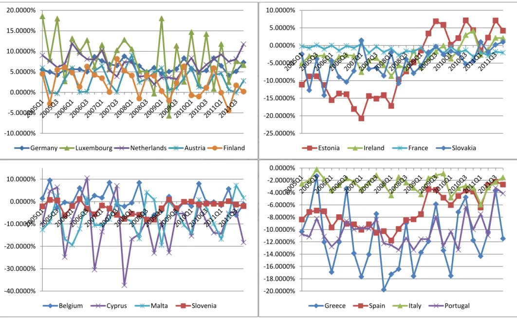
(25) 4 The Empirical Model In this part, we put the collected data into the previous model first and obtain the values of the interest rate sensitivity of output, ℎ’(𝑘𝑎). After comparing the values of ℎ’(𝑘𝑎) in different countries, section 4.4 sets up a panel data regression model to consider what variables might affect the interest rate sensitivity of output. In the end of this section, the result of regression will be used to estimates the out of sample values of ℎ’(𝑘𝑎) in 2011 Q4 and try inferring the appropriate capital requirement policies for the countries in EU-17 individually according to their different macroeconomic environments.. 立. ‧. ‧ 國. 學. 4.1 Data. 政治大. All the data is collected mainly from the Datastream, Eurostat Statistics Database and. sit. y. Nat. European Central Bank (ECB) Database. OECD iLibrary and the database of central. n. al. er. io. banks in the respective countries are also the sources of a part of data. The range of data. v. is within the 17 countries in the European Monetary Union, and the period of data is. Ch. engchi. i Un. from 2005 Q1 to 2011 Q4. The part of calculation and regression in section 4.3 and section 4.5 is composed of data from 2005 Q2 to 2011 Q3, and the part of estimation in section 4.6 also includes the data in 2011 Q4. The detailed description of data is listed in Table 6 and Table 7 in Appendix A.. 4.2 Statistics of Economics Environment in EU-17 4.2.1 Current Account Observing the current account deficits in individual EU-17 from 2005 Q1 to 2011 Q4 in 19.

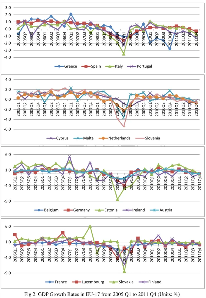
(26) Figure 1, these countries can be classified into four kinds in general. Current account to GDP ratio in Germany, Luxembourg, Netherlands, Austria, and Finland is the first kind of classification. Current accounts in these 5 countries are positive most of the time. Current accounts in Ireland, France, Slovenia and Slovakia are close to zero in recent several quarters. The values in Belgium, Ireland, Cyprus and Malta are volatile. Sometimes they are positive and sometimes negative largely. The last kind of classification is for Greece, Spain, Italy, and Portugal, which keep negative values all the time. They happen to be the nations with or possibly with debt crises. From the graphs, it can be seen that economy in Ireland is not that pessimistic.. 治政大 smaller and has a tendency Although its values are often negative, its deficit is becoming 立 towards zero.. ‧ 國. 學. 4.2.2 Growth Rate of Output. ‧. In Figure 2, the GDP growth rates in EU-17 have similar trends, with declining growth. y. Nat. io. sit. rates from 2005 Q1, experiencing the seriously decline during the financial crisis around. n. al. er. 2008 and 2009, and recovering gradually. However, most of the countries have a. Ch. i Un. v. downward direction again in the recent years. Although having similar trends, the. engchi. growth ratios of these countries can be organized into four groups by their degrees of growth. Greece, Spain, Italy, and Portugal are in the first group, and their growth levels are relatively lowest compared to other countries in most periods. Cyprus, Malta, Netherlands, and Slovenia are in the second relatively lowest group. Ireland, Belgium, Germany, Estonia, and Austria are in the second relatively highest group. The nations with highest levels of growth are France, Luxembourg, Slovakia, and Finland, that have positive or zero growth rates in 2011 Q4.. 20.

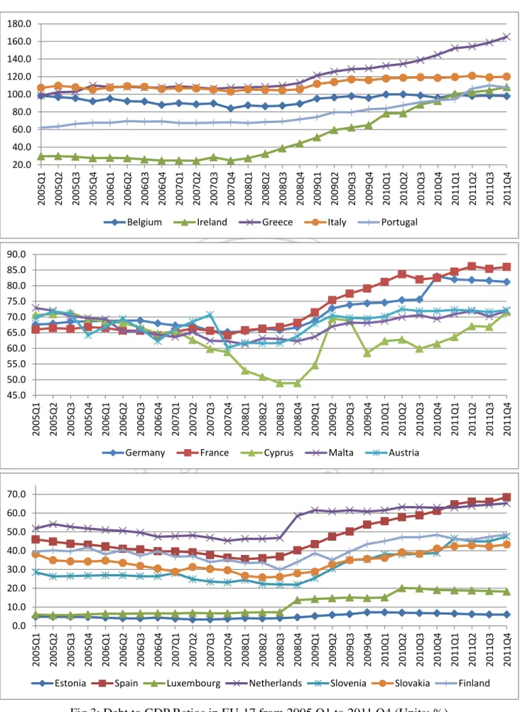
(27) 4.2.3 Debt to GDP Ratio It is observed that in Figure 3, most of the accumulative public debt ratios in EU-17 have positive trends of curves from 2005 Q1 to 2011 Q4. These countries can be categorized into three groups by the debt ratios, which are more than 90%, between 70%-90%, and smaller than 70% in 2011 Q4. Greece, Italy, Ireland, Portugal, and Belgium are in the relatively higher level of debt to GDP ratios, while Spain is in the relatively lower level of debt to GDP ratios. The levels of debt ratios in these countries reflected the countries with higher debt ratios are more vulnerable and prone to involved in the European debt crisis.. 立. 政治大. ‧. ‧ 國. 學. n. er. io. sit. y. Nat. al. Ch. engchi. 21. i Un. v.

(28) 20.0000%. 10.0000%. 15.0000%. 5.0000% 0.0000%. 10.0000%. -5.0000% 5.0000% -10.0000% 0.0000%. 立. -5.0000%. Austria. Finland 0.0000% -2.0000% -6.0000% -8.0000% -10.0000%. n. al. -20.0000%. Ch. i n U. -12.0000%. France. Slovakia. sit. io. -10.0000%. Ireland. y. -4.0000%. Nat. 0.0000%. Estonia. ‧. 10.0000%. Netherlands. er. Luxembourg. ‧ 國. Germany. -25.0000%. 學. -10.0000%. 治政 -15.0000% 大 -20.0000%. v. e n g-14.0000% chi -16.0000%. -30.0000%. -18.0000% -40.0000%. -20.0000%. Belgium. Cyprus. Malta. Slovenia. Greece. Spain. Italy. Fig 1. Current Account to GDP Ratios in EU-17 from 2005 Q1 to 2011 Q4 (Units: %) 22. Portugal.

(29) France. Luxembourg. 23. Slovakia. sit. 2011Q3 2011Q4. 2011Q3. 2011Q4. 2010Q4. 2010Q3. 2010Q2. 2010Q1. 2011Q2. 1.0. 2011Q2. 6.0 2011Q1. Austria. 2011Q1. 2010Q4. 2010Q3. Ireland. 2010Q2. 2010Q1. er. 2009Q4. v. 2009Q4. y. 2009Q3. i Un 2009Q2. 2009Q1. 2010Q4 2011Q1 2011Q2 2011Q3 2011Q4. 2010Q1 2010Q2 2010Q3. 2009Q2 2009Q3 2009Q4. Italy. 2009Q3. Estonia. 2009Q2. engchi. 2009Q1. 2008Q4. Netherlands. 2008Q3. 政治大 2008Q2 2008Q3 2008Q4 2009Q1. 2007Q3 2007Q4 2008Q1. 2006Q3 2006Q4 2007Q1 2007Q2. Spain. 2008Q4. 2008Q2. 2008Q1. 2007Q4. Malta. 2008Q3. Germany. 2008Q2. Ch. 2008Q1. 2007Q4. Belgium 2007Q3. Cyprus. ‧ 國立. 2007Q3. -9.0 2007Q2. al. 2007Q2. 2007Q1. 2006Q4. 2006Q3. -4.0. 2007Q1. 2006Q4. 2006Q3. 2006Q2. 2005Q4 2006Q1 2006Q2. 2005Q1 2005Q2 2005Q3. Greece. 學. 2006Q2. 2006Q1. n. 2006Q1. 2005Q4. io. 2005Q4. 2005Q3. 1.0. Nat. -4.0. 2005Q3. 6.0. ‧. -4.0 2005Q2. -2.0. 2005Q2. -9.0. Finland. Fig 2. GDP Growth Rates in EU-17 from 2005 Q1 to 2011 Q4 (Units: %) 2011Q4. 2010Q1 2010Q2 2010Q3 2010Q4 2011Q1 2011Q2 2011Q3. 2008Q2 2008Q3 2008Q4 2009Q1 2009Q2 2009Q3 2009Q4. 2006Q3 2006Q4 2007Q1 2007Q2 2007Q3 2007Q4 2008Q1. 2005Q1 2005Q2 2005Q3 2005Q4 2006Q1 2006Q2. -2.0. 2005Q1. -1.0. 2005Q1. 3.0. 2.0. 1.0. 0.0. -3.0. -4.0 Portugal. 4.0. 2.0. 0.0. -6.0 Slovenia.

(30) Estonia. Spain. Luxembourg. 24. engchi. 60.0. 50.0. 40.0. 30.0. 20.0. 10.0. 0.0. Netherlands. v. Slovenia 2011Q1 2011Q2 2011Q3 2011Q4. 2011Q1. 2011Q2. 2011Q3. 2011Q4. 2010Q3. 2010Q2 2010Q4. Austria. 2010Q4. 2010Q3. Malta. 2010Q2. 2010Q1. 2009Q3. s2009Q4 ity. Italy. 2010Q1. 2009Q4. er. 2009Q2. 2009Q1. 2008Q4. 2008Q3. Greece. 2009Q2. i Un. 2009Q3. Cyprus. 2009Q1. 2008Q4. 2008Q3. France 2008Q2. 2008Q1. 2007Q4. Ireland. 2008Q2. 70.0. Ch. 2008Q1. al 2007Q3. 2007Q2. 2007Q1. 立. 2007Q4. ‧ 國 2006Q4. 2006Q3. 2006Q2. 2006Q1. 2005Q4. 2005Q3. Belgium. 2007Q3. 2007Q2. 2007Q1. 2006Q4. 2006Q3. 2006Q2. 2006Q1. 2005Q4. 2005Q3. 2005Q2. ‧. n. Germany. 學. io. 2005Q2. 2005Q1. 90.0 85.0 80.0 75.0 70.0 65.0 60.0 55.0 50.0 45.0. Nat. 2005Q1. Slovakia. Fig 3: Debt to GDP Ratios in EU-17 from 2005 Q1 to 2011 Q4 (Units: %). Finland. 2011Q4. 2011Q3. 2011Q2. 2011Q1. 2010Q4. 2010Q3. 2010Q2. 2010Q1. 2009Q4. 2009Q3. 2009Q2. 2009Q1. 2008Q4. 2008Q3. 2008Q2. 2008Q1. 2007Q4. 2007Q3. 2007Q2. 2007Q1. 2006Q4. 2006Q3. 2006Q2. 2006Q1. 2005Q4. 2005Q3. 2005Q2. 2005Q1. 180.0. 160.0. 140.0. 120.0. 100.0. 80.0. 60.0. 40.0. 20.0. Portugal. 政治大.

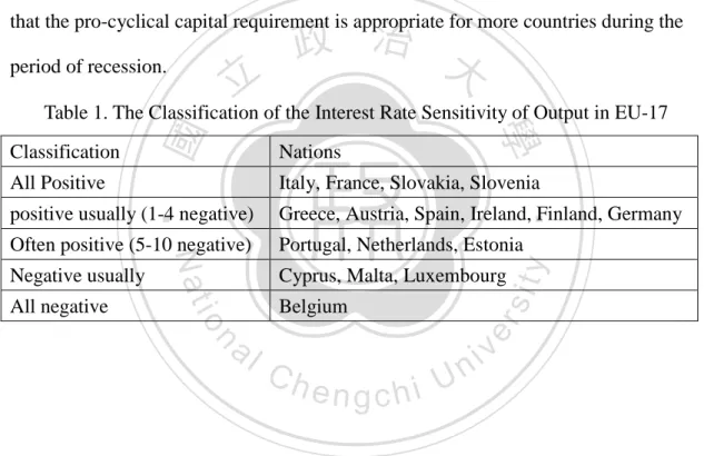
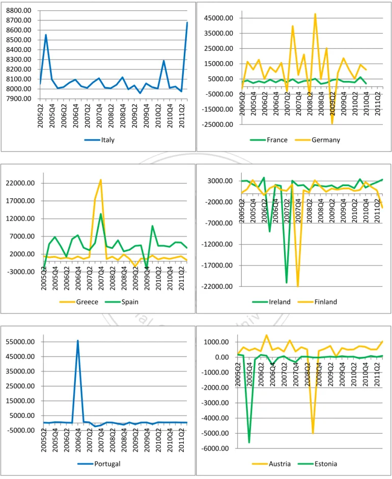
(31) 4.3 Comparison of the Interest Rate Sensitivity of Output between EU-17 Because the adjustment of capital requirement to the per unit change of GDP,. 𝑑𝑘 𝑑𝑌. , is. affected by ℎ′ (𝑘𝑎), the interest rate sensitivity of output, this paper will evaluate the change of capital to per unit change of GDP through the interest rate sensitivity of output.. 治政大 in different countries can organized data into equation (10). After calculated, ℎ (𝑘𝑎) 立 The interest rate sensitivity of output of EU-17 can be calculated by putting the ′. be sorted into five kinds of classification according to their values in Table 1 and are. ‧ 國. 學. graphed in Figure 4 and 5. The detailed values are in Table 8. Large parts of ℎ′ (𝑘𝑎). ‧. in EU-17 are positive. Especially, ℎ′ (𝑘𝑎) are all positive in Italy, France, Slovakia,. sit. y. Nat. and Slovenia. However, ℎ′ (𝑘𝑎) in Cyprus, Malta, and Luxembourg are negative in. io. al. er. general and all negative in Belgium. Italy and Slovenia are relatively least fluctuated. n. within the positive classification, and Cyprus and Malta are relatively least fluctuated. Ch within the negative classification.. engchi. i Un. v. Based on the former equation in section 3.3, we know that the adjustment of 𝑑𝑘. capital requirement to per unit change of GDP (𝑑𝑌) will have the same direction with the interest rate sensitivity of output. Thus, the adjustments of capital requirement to the change of GDP in most of countries are positive, and the ratios in Belgium, Cyprus, Malta, and Luxembourg are negative most of the time. When the interest rate sensitivity of output is positive, this means that the capital requirement should be higher when one economy is growing and lower when one economy is declining. This counter-cyclical capital policy is appropriate for countries 25.

(32) like Italy, France, Slovakia, and Slovenia. The capital requirement should be in the same direction of ℎ′ (𝑘𝑎) in most countries most of the time. On the other side, the capital requirement should be pro-cyclical in Belgium, Cyprus, Malta, and Luxembourg most of the time. When there is a positive growth ratio in one country, the capital requirement should be decreased. Conversely, the capital requirement should be stricter during the period of negative growth ratio. The interest rate sensitivity of output is negative in more countries during the period of 2008 Q3 and 2008 Q4, the financial crisis period. This can be considered. 政治大. that the pro-cyclical capital requirement is appropriate for more countries during the period of recession.. 立. All Positive. 學. Classification. ‧ 國. Table 1. The Classification of the Interest Rate Sensitivity of Output in EU-17 Nations. Italy, France, Slovakia, Slovenia. ‧. Often positive (5-10 negative). Portugal, Netherlands, Estonia. Negative usually. Cyprus, Malta, Luxembourg. sit. Belgium. n. al. er. io. All negative. y. Greece, Austria, Spain, Ireland, Finland, Germany. Nat. positive usually (1-4 negative). Ch. engchi. 26. i Un. v.

(33) 8800.00 8700.00 8600.00 8500.00 8400.00 8300.00 8200.00 8100.00 8000.00 7900.00. 45000.00 35000.00 25000.00 15000.00. 2011Q2. 2010Q4. 2010Q2. 2009Q4. 2009Q2. -15000.00 -25000.00. Italy. France. 立. 17000.00. 2011Q2. 2010Q4. 2010Q2. 2009Q4. -5000.00 -6000.00. Portugal. Austria. Estonia. Fig 4. The Interest Rate Sensitivity of Output in EU-17 from 2005 Q2 to 2011 Q3. 27. 2011Q2. 2010Q4. 2010Q2. 2009Q4. 2009Q2. 2008Q2. 2007Q4. 2007Q2. 2006Q4. -4000.00 2009Q2. 5000.00. 2008Q4. -3000.00. 2008Q2. 15000.00. 2007Q4. -2000.00. 2007Q2. 25000.00. 2006Q4. -1000.00. 2006Q2. 35000.00. 2005Q4. 0.00. 2005Q2. 45000.00. v. 2006Q2. e n g 1000.00 chi. i Un 2005Q4. Ch. 2005Q2. n. al. Finland. er. Ireland. 55000.00. -5000.00. y. -22000.00. sit. 2011Q2. 2010Q4. 2010Q2. -17000.00. Spain. io. Greece. 2009Q4. 2009Q2. ‧ 國 2008Q4. 2007Q4. 2007Q2. 2006Q4. 2006Q2. 2005Q4. -12000.00. Nat. 2005Q2. -7000.00. ‧. 2000.00. 2008Q2. 7000.00. -2000.00. 學. 12000.00. -3000.00. 政治 3000.00 大 2005Q2 2005Q4 2006Q2 2006Q4 2007Q2 2007Q4 2008Q2 2008Q4 2009Q2 2009Q4 2010Q2 2010Q4 2011Q2. 22000.00. Germany. 2008Q4. 2008Q4. 2008Q2. 2007Q4. 2007Q2. 2006Q4. 2006Q2. 2005Q4. 2005Q2. -5000.00. 2005Q2 2005Q4 2006Q2 2006Q4 2007Q2 2007Q4 2008Q2 2008Q4 2009Q2 2009Q4 2010Q2 2010Q4 2011Q2. 5000.00.

(34) 650.00. er. al Ch. Luxembourg. sit. engchi. 28. i Un. Belgium. 2010Q2. 2009Q4. 2009Q2. 2008Q4. 2008Q2. 2007Q4. 2007Q2. 2006Q4. 2006Q2. 2005Q4. 2005Q2. 2011Q2. -1600.00. 2011Q2. -1400.00. 2010Q4. -1200.00. 2010Q4. 2010Q2. 2009Q4. 政治大. 4000 3500 3000 2500 2000 1500 1000 500 0 2009Q2. Malta. 2008Q4. -2000.00. 2008Q2. -350.00. 2007Q4. -1800.00. y2007Q2. -250.00. 2006Q4. 50.00. 2006Q2. 2011Q2. 2010Q4. 2010Q2. 2009Q4. 2009Q2. 2008Q4. 2008Q2. 2007Q4. 2007Q2. -1000.00. 2005Q4. 2005Q2. 立. 2011Q2. 12000.00. 2010Q4. 750.00. 2010Q2. 2000.00. 2009Q4. -38000.00. 2009Q2. Cyprus. 2008Q4. ‧ 國. -28000.00. 2008Q2. -18000.00. 2007Q4. 2007Q2. 2006Q4. -800.00. ‧. n. 2006Q4. 2006Q2. 2005Q4. 150.00. 學. io. 2006Q2. -8000.00. 2005Q4. 2005Q2. -150.00. 2005Q2 2005Q4 2006Q2 2006Q4 2007Q2 2007Q4 2008Q2 2008Q4 2009Q2 2009Q4 2010Q2 2010Q4 2011Q2. -50.00. Nat. 2005Q2. 250.00. Slovakia. v. 550.00. 450.00. 350.00. 250.00. 150.00. Slovenia. Fig 5. The Interest Rate Sensitivity of Output in EU-17 from 2005 Q2 to 2011 Q3 (continued).

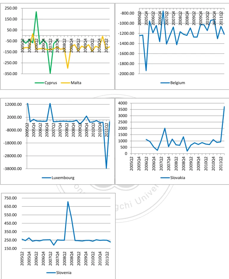
(35) 4.4 The Method of Regression In this model, ℎ’(𝑘𝑎) of EU-17 are calculated from 2005 Q2 to 2011 Q3. The model uses the regression of panel least squares to analyze how ℎ’(𝑘𝑎) change across different countries and different periods on the same time. Before carrying out the regression of panel data, there is a unit root test for the considered variables in the regression in section 4.4.1.. 4.4.1 Unit Root Test. 政治大 There are six variables which need a unit rood test before we formally run the 立. regression. The result of the tests in Table 2 reveals that the debt to GDP ratio is. ‧ 國. 學. un-stationary and is in the situation of unit root. The problem can be avoided by using. ‧. the first difference of these three variables as the new variables in the latter regression. sit. y. Nat. model, because the first difference of debt to GDP ratio is stationary after they. io. al. n. difference is in Table 3.. er. changed their original levels into first difference. The result of the test with first. Ch. engchi. 29. i Un. v.

(36) Table 2. Panel Unit Root Tests on the Original Data Period: from 2005 Q2 to 2011 Q3 Null Hypothesis : Unit root (assumes individual unit root process) Government Money supply DEBT/GDP. Public Ratio. expenditure. Trade Openness. elasticity of output elasticity of output Statistics P-value Statistics P-value Statistics P-value Statistics P-value Statistics P-value Im, Pesaran 5.9643. 1.0000. -13.7797. 0.0000. 13.6923. 0.9992. 231.007. 0.0000. -16.3643. 0.0000 -9.05235. 0.0000. -3.11017. 0.0009. 0.0000. 65.3137. 0.0010. 0.0000. 47.274. 0.0647. and Shin W-stat ADF Fisher Chi-square. 立. PP -. Chi-square. 1.0000. 278.715. ‧ 國. 9.9291. 0.0000. 239.358. 0.0000. 308.523. 學. Fisher. 政218.574治0.0000大143.632. ‧. Table 3. Panel Unit Root Tests on the Variables with First Difference Period: from 2005 Q2 to 2011 Q3. sit. y. Nat. io. al. Im, Pesaran and Shin W-stat. Statistics. -5.7948. P-value. 0.0000. n. D(DEBT/GDP). Ch. er. Null: Unit root (assumes individual unit root process) ADF - Fisher Chi-square. e n g c0.0000 hi U 91.6443. 30. n. iv. PP - Fisher Chi-square 89.4419 0.0000.

(37) 4.5 Variables, Explanations, and Results of Regression To find the variables that possibly affect the value of ℎ’(𝑘𝑎), this model considers six variables, including debt to GDP ratio, fiscal policy ratio, the elasticity of IS curve, the elasticity of LM curve, trade openness, money supply elasticity of output. 𝐷𝑒𝑏𝑡 ℎ’(𝑘𝑎) = 𝐶(1) + 𝐶(2) ∗ 𝑑 ( ) + 𝐶(3) ∗ 𝐹𝑖𝑠𝑐𝑎𝑙 𝑝𝑜𝑙𝑖𝑐𝑦 𝑟𝑎𝑡𝑖𝑜 + 𝐶(4) 𝐺𝐷𝑃 ∗ 𝑀𝑜𝑛𝑒𝑦 𝑠𝑢𝑝𝑝𝑙𝑦 𝑒𝑙𝑎𝑠𝑡𝑖𝑐𝑖𝑡𝑦 𝑜𝑓 𝑜𝑢𝑡𝑝𝑢𝑡 + 𝐶(5) ∗ 𝐺𝑜𝑣𝑒𝑟𝑛𝑚𝑒𝑛𝑡 𝑒𝑥𝑝𝑒𝑛𝑑𝑖𝑡𝑢𝑟𝑒 𝑒𝑙𝑎𝑠𝑡𝑖𝑐𝑖𝑡𝑦 𝑜𝑓 𝑜𝑢𝑡𝑝𝑢𝑡 + 𝐶(6). 政治大. ∗ 𝑇𝑟𝑎𝑑𝑒 𝑂𝑝𝑒𝑛𝑛𝑒𝑠𝑠. 立. ‧ 國. 學. 4.5.1 Variables. a. Debt to GDP ratio6:. ‧. The accumulated public debt relative to GDP ratio.. Nat. sit. y. b. Fiscal policy ratio7:. n. al. er. io. The ratio that calculates how much weight the fiscal policy stands for in total effects of fiscal and monetary policy.. Ch. engchi. i Un. v. c. Money supply elasticity of output:. The elasticity to calculate how much percent of GDP will vary when money supply change one percent. d. Government expenditure elasticity of output:. 6 Debt. with first difference.. GDP |G𝑒 | 7 |G𝑒 |+|. . The effect of monetary policy is estimated from LM curve.. dm | 𝐿𝑦. mS = 𝐿(𝑌, 𝑟), 𝐿𝑦 𝑑𝑦 + 𝐿𝑟 𝑑𝑟 = 𝑑mS , 𝑑𝑦 = 𝑑𝑦 =. 𝑑mS 𝐿𝑦. 𝑑mS −𝐿𝑟 𝑑𝑟 𝐿𝑦. . 31. . Considering 𝑑𝑟 is zero, so the move in.

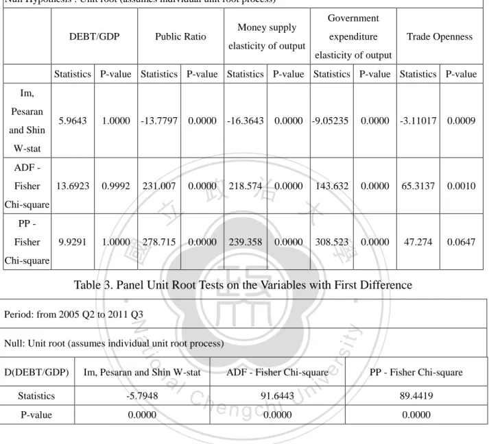
(38) The elasticity of how much percent of GDP will be affected when the government expenditure changes 1%. e. Trade openness8: Trade openness is the sum of export and import to GDP ratio. This ratio represents the level of openness to accept the international trades in a country.. 4.5.2 Results and Explanation The outcome of the panel data is listed in Table 4. Table 4. The Result of Panel Data Regression Dependent Variable: ℎ’(𝑘𝑎) Method: Panel Least Squares Sample: 2005 Q2 – 2011 Q3 Cross-sections included: 17 Total panel (unbalanced) observations: 390. 政治大. 學. ‧ 國. 立. n. al. er. io. sit. y. Nat. ***. t-Statistic 4.369856 -0.47748 -1.48815 0.401526. ‧. Variables Coefficient Std. Error Intercept 8159.225 1867.161 Debt to GDP ratio -77.9641 163.283 Fiscal policy ratio -2674.61 1797.277 Money supply elasticity of output 6.672881 16.6188 Government expenditure -282.46 341.288 elasticity of output Trade openness -37.664 7.470726 R-squared 0.071263 Adjusted R-squared F-statistic 5.892967 Prob(F-statistic) Mean dependent var 1740.273 S.D. dependent var. Ch. engchi U. v ni. Prob. 0.0000*** 0.6333 0.1375 0.6883. -0.82763 0.4084 -5.04155 0.0000*** 0.05917 0.000029 8081.261. indicate coefficient estimates significantly different from zero at the 1% level.. a. Debt to GDP ratio When one country is with higher ratio, its interest rate sensitivity of output is 𝑑𝑘. smaller. Hence, the adjustment of capital requirement to per unit change of GDP (𝑑𝑌) should be larger.. 8. Trade openness is calculated by. (X+M) GDP. . 32.

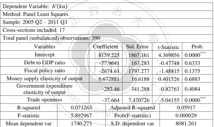
(39) b. Fiscal policy ratio When the fiscal policy ratio is higher or the monetary policy ratio is lower, its interest rate sensitivity of output is smaller. Hence, the adjustment of capital 𝑑𝑘. requirement to per unit change of GDP (𝑑𝑌) should be larger. c. Money supply elasticity of output If the money supply elasticity of output is larger, its interest rate sensitivity of output will be larger and the adjustment of capital requirement to per unit change of 𝑑𝑘. GDP (𝑑𝑌) should be smaller.. 政治大. d. Government expenditure elasticity of output. 立. If the government expenditure elasticity of output is larger, its interest rate. ‧ 國. 學. sensitivity of output is smaller. If the interest rate sensitivity of output is smaller, the 𝑑𝑘. sit. y. Nat. f. Trade openness. ‧. adjustment of capital requirement to per unit change of GDP (𝑑𝑌) should be larger.. io. al. er. When one country is more open-minded to accept the international trade, its. v. n. interest rate sensitivity of output will be smaller. That is, the adjustment of capital. Ch. e n𝑑𝑘g c h i. i Un. requirement to per unit change of GDP (𝑑𝑌) should be larger.. 4.6 Estimation and Policy Suggestion To estimate the adjustment of capital requirement to per unit change of GDP, ℎ’(𝑘𝑎), in 2012 Q4, the regression in section 4.5 is used to calculate the values of ̂ . Most of the ℎ′(𝑘𝑎) ̂ , which are graphed in Figure 6, are positive in 2012 Q4. ℎ′(𝑘𝑎) ̂ in Luxembourg, Ireland, Slovakia, Estonia, and Malta are negative. Only ℎ′(𝑘𝑎) Therefore, it can be suggested that policy in those nations with debt crises should be 33.

(40) different. Adjust of capital requirement should be counter-cyclical in Italy, Greece, Spain, and Portugal, but pro-cyclical in Ireland during 2011 Q4.9 During 2011 Q4, the change of capital requirement to the change of GDP is both positive and largest in Belgium. It is becoming smaller in Slovenia, Netherlands, Austria, Germany, Finland, Portugal, Spain, Italy, and Greece. The positive and smallest one is the value of France. In the pro-cyclical countries, the change of capital requirement to the change of GDP is smallest in Luxembourg, then becoming larger in Ireland, Slovakia, Estonia, and Malta.. 立. 政治大. ‧. ‧ 國. 學. n. er. io. sit. y. Nat. al. 9. Ch. engchi. i Un. v. Cyprus is not included in this estimation because some data is still not available in 2011 Q4. 34.

(41) 5000 4000 3000 2000 1000 0 -1000 -2000 -3000 -4000. Neth Luxe Belgi Slove Austri Germ Finlan Portu Greec Franc Irelan Slova Eston Spain Italy Malta erlan mbou um nia a any d gal e e d kia ia ds rg. h'(ka) 21.17 47.49 198.9 1701 2210 2871 3122 3232 3454 4126 4351 -2786 -1965 -1184 -626 -556. 立. 政治大. ‧. ‧ 國. 學. 10.00% 8.00% 6.00% 4.00% 2.00% 0.00% -2.00% -4.00% -6.00% -8.00% -10.00%. sit. y. Nat. Neth Luxe Belgi Slove Austri Germ Finla Portu Greec Franc Irelan Slova Eston Spain Italy Malta erlan mbou um nia a any nd gal e e d kia ia ds rg. io. 0.1. al. n. 0.15. er. Growth Rate (%) 7.87% -3.41 6.88% -1.27 -0.28 4.55% 0.98% 7.69% 4.39% -8.62 5.06% 7.68% -2.58 -2.75 2.43% -4.60. Ch. engchi. i Un. v. 0.05 0 -0.05 -0.1 -0.15. Neth Luxe Belgi Slove Austri Germ Finlan Portu Greec Franc Irelan Slova Eston Spain Italy Malta erlan mbou um nia a any d gal e e d kia ia ds rg. CA -0.01 -2.04 11.73 2.791 0.073 0.174 -4.15 -2.68 -1.53 -11.4 -2.07 6.634 2.065 0.968 4.196 1.627. Fig 6. Estimation of the Interest Rate Sensitivity of Output, Growth Rate (%), and Current Account to GDP Ratio (%) in EU-17 in 2011 Q4 35.

(42) Observing the relationship between ℎ’(𝑘𝑎) and current account, all the five pro-cyclicality countries have positive values of current account. However, there are positive or negative values of current account in counter-cyclicality countries. Combining the estimation of ℎ’(𝑘𝑎) and Growth rate, the suggestion of policies for capital requirement in EU-17 are listed in the Table 5. Table 5. Suggestion of Policies for Capital Requirement in 2011 Q4. Counter-cyclicality policy for capital. Negative GDP growth rate in. 2011 Q4. 2011 Q4. Raise the adjustment of capital requirement in Italy, Spain, Portugal, Belgium, Netherlands, Finland, and France.. Lower the adjustment of capital requirement in Greece, Germany, Slovenia, and Austria.. Lower the adjustment of capital requirement in Luxembourg and Estonia.. Raise the adjustment of capital requirement in Ireland, Slovakia, and Malta.. ‧. ‧ 國. 立. 政治大. 學. io. sit. y. Nat. n. al. er. Pro-cyclicality policy for capital. Positive GDP growth rate in. Ch. engchi. 36. i Un. v.

(43) 5 Conclusion The results of the model show that the standard of capital requirement should not be comprehensive across EU-17. The adjustment of capital requirement should be considered thoroughly for the various macroeconomic environments in different countries and during different periods. For pro-cyclicality countries, when the economy is in prosperity, the capital requirement should be decreased. However, the capital requirement should be stricter during the period of economic recession. For the counter-cyclicality countries, the. 政治大. situations will be converse. Furthermore, if we have collected the updated data, then. 立. we could obtain the estimation in every period by the established model. For example,. ‧ 國. 學. the regression model suggests that in 2011 Q4 the capital requirement should be. ‧. pro-cyclical in Luxembourg, Ireland, Slovakia, Estonia, and Malta; counter-cyclical in other EU-17 (except for the Cyprus). For those countries involved in the debt crisis,. y. Nat. er. io. sit. Italy, Spain, Portugal, and Ireland should raise the adjustment of capital requirement, and Greece should lower the adjustment of capital requirement.. n. al. Ch. engchi. 37. i Un. v.

(44) Appendix A. Table 6. The Descriptions of Data Variable. Description. Y. Gross domestic product. Datastream. C. Final consumption expenditure of households. Datastream. I. Gross fixed capital formation. Datastream. X. Exports of goods and services. M. Imports of goods and services. G(consumption). Final consumption expenditure of general government. G(expenditure). Total general government expenditure. Eurostat. M𝑆. Money supply 2. Datastream. CPI. Harmonized European Union Basis (2005=100). Euro. Index. Current account, Income (net). n. Current account, Current transfers (net). 38. OECD iLibrary. Percentage. sit. F. engchi. Datastream/ Eurostat/. er. Current account (net). Ch. Datastream. y. ‧ 國. CA. io. S. Gross saving (substitute: Net saving in Luxembourg and Malta). Datastream. ‧. Nat. Total tax revenue of the general government. Datastream. Eurostat. interbank). T. TR. Millions of. 政治大. Interbank interest rate- 3 month (if not available, treasury or deposit rate are substituted for. al. Source. 學. R. 立. Unit. i Un. v. Millions of Euro. ECB. Eurostat Eurostat Eurostat Eurostat.

(45) Table 7. The Descriptions of Interest Rates (unit: percentage) Nation. Description. Source. Austria. OE INTERBANK OFFERED RATE: THREE MONTH. Datastream. Belgium. BG THREE MONTH INTERBANK OFFERED RATE (EP). Datastream. France. FR PIBOR / EURIBOR - 3-MONTH (MTH.AVG.). Datastream. BD FIBOR - 3 MONTH (MTH.AVG.). Datastream. FN HELIBOR - 3 MONTH (MTH.AVG.). Datastream. Netherlands. NL INTERBANK THREE MONTH: OFFERED RATE (EP). Datastream. Greece. GR THREE MONTH INTERBANK RATE (EP). Datastream. Ireland. IR INTERBANK OFFERED RATE - 3 MONTH (EP). Datastream. 立. 政治大. 學. IT INTERBANK DEPOSIT RATE-AVERAGE ON 3-MONTHS DEPOSITS. Spain. ES INTERBANK RATE - 3 MONTH. y. Nat. Datastream. (WEIGHTED AVERAGE, EP). Cyprus. INTERBANK 1-6 MONTH INTEREST RATE. Estonia. TALIBOR Interbank- 3 month. n. er. PT LISBON INTERBANK OFFER RATE - 3 MONTH (EP). io. Portugal. al. Luxembourg Malta. Ch. engchi. Datastream. ‧. Italy. sit. Finland. ‧ 國. Germany. i Un. MFI interest rates - Deposits MA TREASURY BILL RATE - 3 MONTH. Slovakia. Interbank rate-3 month. Slovenia. SJ TREASURY BILL RATE - 3 MONTH (EP). v. Datastream. Central Bank of Cyprus Central Bank of Estonia Eurostat Datastream OECD iLibrary. 39. Datastream.

(46) Table 8. The Results of Simple Regressions. Finland. France. Germany. Malta. Netherlands. Portugal. Slovakia. Slovenia. Spain. 632.7606. -387.1018. (P-value). (0.4826). (0.0319). (0.0033). (0.0000). (0.0000). (0.0036). (0.0041). (0.5653). Coefficient. 0.1114. 20.6836. 192.6522. 1.1487. 0.0176. 0.1815. 861.7395. -387.4431. (P-value). (0.0203). (0.0630). (0.2391). (0.0000). (0.0000). (0.2204). (0.0851). (0.5348). Coefficient. 0.7357. 2377.1132. 49.6110. 0.4340. 52.2010. -0.6040. 176.5300. 66.6248. (P-value). (0.0000). (0.0229). (0.4022). (0.0000). (0.0000). (0.3739). (0.5903). (0.8854). Coefficient. 0.7569. -0.3683. 81.4458. 0.7517. 0.0137. 0.1829. -23.9509. 28.7394. (P-value). (0.0000). (0.5841). (0.0110). (0.0000). (0.0000). (0.0305). (0.2539). (0.0199). Coefficient. 0.5143. -33.8418. 330.1788. 0.5745. 0.0333. 0.0906. 697.6792. -106.8312. (P-value). (0.0021). (0.0000). (0.0002). (0.0000). (0.0000). (0.3635). (0.0007). (0.8772). Coefficient. 0.2455. -210.5349. 2007.7071. 0.1111. 4088.7260. -2022.6728. (P-value). (0.0003). (0.0000). (0.0415). (0.0000). (0.6436). Coefficient. 0.3262. -366.7757. 0.3657. 5795.3632. -2742.0517. (P-value). (0.0054). (0.0000). (0.0389). (0.0000). (0.0000). (0.0000). (0.0000). (0.5426). Coefficient. 0.7606. -45.6756. 910.7447. 0.3754. 0.0605. -0.1643. 767.4850. 297.5160. (P-value). (0.0001). (0.0003). (0.0000). (0.0002). (0.0000). (0.4116). (0.1237). (0.5273). Coefficient. 0.2294. -65.4263. 1714.0339. 0.2871. 0.0334. 0.5223. 195.1559. 556.2931. (P-value). (0.0208). (0.2336). (0.0000). (0.0173). (0.1951). (0.0841). (0.7552). (0.5073). Coefficient. 0.0451. -357.0801. 2310.3225. 0.6773. 0.0446. -0.3800. 5508.1058. 344.8150. (P-value). (0.5640). (0.0000). (0.0000). (0.0000). (0.0000). (0.0005). (0.0000). (0.9058). Coefficient. 0.3370. 139.9829. 71.3167. 1.5734. 0.0054. 4.0476. 4945.2658. -11.7347. (P-value). (0.0000). (0.3365). (0.0000). (0.5529). (0.4485). (0.4709). (0.9132). Coefficient. 0.4997. 15.0612. 1786.3795. -4.8768. (P-value). (0.0001). (0.0004). (0.0001). (0.9162). Coefficient. 0.2071. -64.5517. 654.9895. 1.2933. 0.0636. 0.0699. 1708.7932. -38.8938. (P-value). (0.0007). (0.0246). (0.0116). (0.0000). (0.0000). (0.5834). (0.0095). (0.9628). Coefficient. 0.1914. -12.6566. 292.6725. 0.6038. 0.0374. -0.1033. 206.1557. 112.6440. (P-value). (0.1281). (0.1222). (0.0000). (0.0000). (0.0000). (0.3283). (0.0826). (0.6656). Coefficient. 0.7730. -8.9003. 145.6630. 0.8802. 0.0124. 0.1496. 213.0344. 18.4851. (P-value). (0.0000). (0.0001). (0.0278). (0.0000). (0.0000). (0.0405). (0.0154). (0.9116). Coefficient. 0.9820. -2.3984. 135.1240. 0.8671. 0.0097. 0.0581. 146.9495. 35.6243. (P-value). (0.0000). (0.0000). (0.0002). (0.0000). (0.0000). (0.1721). (0.0000). (0.5112). Coefficient. 0.3332. -333.2026. 5590.0363. 0.2928. 0.0712. -0.0028. 1454.9750. -754.1274. (P-value). (0.0002). (0.0000). (0.0000). (0.0045). (0.0000). 0.9694). (0.0592). (0.2690). 立. io. Luxembourg. 0.4623. Nat. Italy. 0.0786. al. (0.0000). 0.4123 0.0513 治政 (0.0137) (0.0000) (0.0000) 大0.0383 1931.2062 0.9380. v ni. C h9.4137 1.0870 U 0.0266 en hi (0.3327) (0.0302)g c(0.0000) (0.0000) 0.5104. 40. ‧. Ireland. 0.6876. 學. Greece. 295.3604. y. Estonia. -43.2671. sit. Cyprus. -0.0544. er. Belgium. Coefficient. n. Austria. 𝒇. ∆𝑩 ̂. Results. ‧ 國. Nation.

(47) Table 9. Values of the Interest Rate Sensitivity of Output (Unit: Index) Ireland. Finland. Germany. Portugal. 188.56. -2590.64 2995.83. 195.30. -1402.90. 253.19. Netherlands 9764.94. 1111.12. 658.72. 4847.39. 3061.09. 1070.93. 16394.83. 99.47. 1261.21. 447.44. 6848.90. 2215.25. 3227.58. 11200.71. 560.92. 581.41. 4316.51. 1544.83. 1224.61. 17643.51. 1040.82. 397.97. 1282.73. 3823.17. 632.14. 1452.48. 6241.33 -8963.29. 1266.92. 252.34. 1338.96. 480.66. 7341.53. 2073.49. 253.98. 669.61. 620.47. 3821.26. 1840.50. 1023.94. 254.84. 1172.19. 372.94. 4880.27. 2008.53. 190.55. 17570.19 1108.31. 2381.56. 548.65. 252.91. 22959.89. 383.44. 13364.26 1907.53 -22242.99 7655.16. 8013.59. 3732.64. 1146.29. 249.11. 644.89. 665.33. 4181.29. 2050.74. 827.59. 21160.91. 8006.79. 4050.06. 696.12. 249.25. 1279.59. 521.77. 3691.84. 865.82. 278.03. -6120.84. 8043.23. 5150.57. 658.92. 706.95. 368.24. -5001.19 5924.60. 2073.04. 3195.23. 47815.69. 2008Q4. 8119.49. 1804.14. 1329.28. 513.10. 1927.90. 416.89. 2780.76. 1844.72. 1692.07. 2009Q1. 7997.23. 2505.16. 197.68. 245.04. 686.70. 559.23. 1691.60. 453.13. 2009Q2. 8036.56. 4241.60. 671.24. 243.53. -1451.70. 749.49. 4328.14. 1962.12. 1217.38 -24163.89. 2009Q3. 7957.07. 4907.77. 851.70. 239.29. 769.98. Nat. 3222.65. 46.85. 4483.08. 1256.59. 957.21. 2009Q4. 8057.16. 3191.21. 723.75. 246.88. 637.52. 611.20. 2010Q1. 8019.50. 3181.93. 871.66. 247.11. 1621.63. 498.43. 2010Q2. 8004.01. 2741.63. 756.36. 236.91. 504.40. 516.47. 2010Q3. 8287.81. 6264.07. 718.77. 254.61. 989.39. 2010Q4. 8011.55. 2047.23. 1106.15. 247.08. 660.96. 2011Q1. 8024.77. NA. 881.37. 249.94. 1051.79. 2011Q2. 7974.21. NA. 929.74. 248.52. 2011Q3. 8678.11. NA. 3719.94. 228.31. Average. 8089.77. 3546.45. 985.78. 273.73. Std. 164.77. 1119.18. 700.35. 101.71. Slovakia. Slovenia. Greece. Austria. 2005Q2. 8053.16. 3104.95. NA. 261.12. 1425.23. 2005Q3. 8552.26. 4034.73. NA. 244.64. 2005Q4. 8096.53. 2332.69. NA. 276.46. 2006Q1. 8007.67. 3552.81. NA. 237.22. 781.99. 2006Q2. 8018.98. 2583.86. 1117.52. 246.44. 2006Q3. 8064.88. 4587.59. 955.23. 240.98. 2006Q4. 8094.71. 2812.11. 519.43. 2007Q1. 8027.89. 4541.20. 254.88. 2007Q2. 8010.70. 2938.65. 2007Q3. 8066.72. 2007Q4. 8109.49. 2008Q1 2008Q2 2008Q3. Spain. Malta. 177.80. -40.52. -118.87. LuxemBelgium bourg 16951.81 -1243.90. 11903.92. 120.55. -70.47. -109.20. -1500.23 -1232.67. 596.99. -5603.67. -37.80. -113.71. 418.28. -1937.58. 546.84. -2977.45. -155.10. -66.16. 16.52. -989.05. -952.69. 245.11. -97501.17. 156.68. 217.67. -124.67. -1020.33 -1187.08. 178.40. 1730.81. 105.10. -79.56. -120.75. -1168.63 -1041.62. 1930.56. 9487.00. 55842.68. -386.75. -495.10. -39.14. -117.57. -1036.75 -1361.78. 931.80. 15637.03. 769.03. 6947.17. -36.06. -73.05. -127.61. 12956.43 -753.35. 3135.74 -21074.86. 673.43. -3040.65. 480.76. 994.22. 75.47. -344.94. -127.08. -1480.48 -1409.89. 5108.41. 2188.71. 39819.44 -2304.94. 1639.35. -172.40. -73.69. -121.13. -1317.03 -1235.61. 1172.18. -320.68. -41.90. -104.40. -1128.10 -1072.07. 382.16. 245.45. 42.65. NA. -126.24. -1005.61 -1422.28. 338.20. 2465.93. 35.47. NA. -115.07. -1137.01 -1166.03. -459.63. -136.32. -12.35. NA. -298.85. -1281.48 -1215.77. 4939.53. -1142.46. -154.35. -16.03. NA. -100.17. -1209.22 -1238.07. 25247.51. 378.14. 479.33. 14.79. NA. -83.57. -323.39. -871.80. 3588.17. 42.46. NA. -140.43. -3234.63 -1271.43. 315.82. 1001.79. 11.24. NA. -96.95. -775.91. 1092.64. 72.98. NA. -111.69. 2932.57 -1025.40. 729.04. 2010.04 1234.96 18655.47 401.68 a-2162.84 9962.97 i v -738.85 l C 1975.11 1279.96 11158.60 n 4377.42 h1298.95 648.90 5111.44 548.96 U i e h n c g 4368.91 3458.02 889.92 14317.72 396.07. 688.45. 4091.35. 1422.22. 2737.23. 11157.72. 397.19. 513.39. 5343.55. 2169.79. 1633.13. NA. 443.76. 1410.49. 521.82. 5273.74. 2714.66. 791.96. NA. 340.38. 1041.45. 3788.47. 3335.24. -3319.59. NA. 2361.75. 375.81. 4514.36. 870.69. 179.10. 11714.53. 5256.52. 1109.85. 3052.88. 4936.67. 4645.89. 政治大. n. 41. ‧. io. 8909.18. -1559.34. er. 3085.66. 學. ‧ 國. 4998.42. Cyprus. 12852.57. 立. -327.42. Estonia. y. France. sit. Italy. -1091.31 -1271.83. 1137.09. 32.43. NA. -83.17. -1821.15 -1025.96. 1612.02. 43.76. NA. -143.39. -1631.60 -1142.75. 941.88. -57.68. NA. -98.24. -539.05. -940.77. 1056.21. -10.63. NA. -110.08. -1952.65. -925.58. 2995.80. 85.96. NA. -7.07. 321.31. 1344.96. 27.60. NA. -120.29 -37638.54 -1060.25. 329.29. 945.75. 95.09. NA. -102.58. -1499.92 -1215.87. 2159.69. -1826.90. -220.76. -59.05. -111.78. -1243.34 -1182.49. 14225.20 10761.38 19376.33 1085.91. 120.91. 51.04. -1895.04 -1303.28. 8514.43. 216.99.