增進IEEE 802.16 網狀分散協同排程網路的效能

(1)

國

立

交

通

大

學

資訊科學與工程研究所

博

士

論

文

增進 IEEE 802.16 網狀分散協同排程網路的效能

Performance Enhancements of the IEEE 802.16 Mesh Coordinated

Distributed Scheduling Mode Network

研究生：林志哲

指導教授：王協源教授

(2)

增進 IEEE 802.16 網狀分散協同排程網路的效能

Performance Enhancements of the IEEE 802.16 Mesh Coordinated

Distributed Scheduling Mode Network

研究生：林志哲 Student：Chih-Che Lin

指導教授：王協源博士 Advisor：Dr. Shie-Yuan Wang

國立交通大學

資訊科學與工程研究所

博士論文

A Dissertation

Submitted to Institute of Computer Science and Engineering College of Computer Science

National Chiao Tung University in partial Fulfillment of the Requirements

for the Degree of Doctor of Philosophy

in

Computer Science

July 2010

Hsinchu, Taiwan, Republic of China

(3)

增進 IEEE 802.16 網狀分散協同排程網路的效能

學生: 林志哲指導教授: 王協源教授

國立交通大學資訊科學與工程研究所

摘要

無線網狀網路為新一代可節省成本的骨幹傳輸網路 (Backbone Relay Network) 解決方案。而 IEEE 802.16 網狀分散協同排程網路 (Mesh Coordinated Distributed Scheduling Network)為下一世代無線網狀網路的候選方案之一。此一新世代的網路具有「無封包碰撞」的特性，與傳統的以 802.11 為基礎的無線網狀網路有非常大的差異。在此篇論文裡，我們提出了數個提升此一新網路效能的方案，包括了提升其控制訊息排程效率的方案與增加其服務品質 (Quality of Service) 的方案。除此之外，針對此網路的初始化流程。我們發現了一個網路節點在任意拓墣 (General Topology) 裡，可能會初始化失敗的問題，並且提出解決的方案。在此篇論文裡，我們以理論分析與模擬的方式來評估所提出的方案的效能。我們的理論分析與模擬結果皆顯示我們所提出的各項方案能有效地提升 IEEE 802.16 網狀分散協同排程網路的效能。關鍵字: 無線網狀網路、802.16、分散式排程

(4)

Performance Enhancements of the IEEE 802.16 Mesh

Coordinated Distributed Scheduling Mode Network

Student: Chih-Che Lin Advisor: Dr. Shie-Yuan Wang

Institute of Computer Science and Engineering

College of Computer Science

National Chiao Tung University

ABSTRACT

The Wireless Mesh Network (WMN) is a cost-effective solution for backbone

networks in both metropolitan and rural areas and can be used as temporary

broadband access for emergent and tactic purposes. Without the need of wires,

WMNs are easy to deploy and reconstruct to satisfy the dynamic needs. The

IEEE 802.16 mesh CDS-mode network is a candidate of next-generation WMNs,

which provides the “collision-free” property unique to traditional IEEE 802.11

based WMNs.

In this dissertation, we propose several schemes for this new network to enhance

its scheduling efficiency on the control plane and its QoS support on the data

plane. In addition, we also point out the issues of network initialization of this

network on random topologies and propose a scheme to solve these issues. The

performances of our proposed schemes are evaluated using both analyses and

simulations. Our analytical and numerical results show that our proposed

schemes can significantly enhance the performance of the IEEE 802.16 mesh

CDS-mode network and benefits upper-layer applications.

(5)

iii

致謝

回顧我的求學生涯，已在交通大學裡待了十二個年頭。這一路艱辛的研究旅程，我要感謝指導教授王協源老師的悉心栽培。在他的教導之下，我於研究、思考、專案管理以及文章撰寫都逐漸地成熟。我也要感謝我的校內校外論文指導委員 (林一平院長、曾煜棋副院長、曾建超所長、清華大學許建平教授、成功大學郭耀煌教授，以及台灣大學林風教授等) 給予我的論文具有建設性的建議，使我能在畢業之際發掘自己的缺點，加以改進，成為一個更加成熟的研究者。我亦要感謝所有在實驗室裡同甘共苦的周智良學長與歷屆學長學弟妹，沒有你們的共同參與及集思廣益，我的許多研究將不會那麼順利完成。在這漫長的研究歷程，我要感謝我父親與母親的支持與體諒。感謝他們無私地支持著我完成這一個漫長的學業歷程，感謝他們即便處於最艱困的時刻都仍努力成為我生活上的後盾。沒有他們在生活上的全力支持，容忍我將人生的第一個黃金階段花在十年的學業上，就沒有今天取得博士學位的我。此外，我要感謝我的外公與各位阿姨，感謝你們這麼多年來默默地支持我與母親，使得我能在這一生活艱困的時刻，仍能心無旁騖於研究與學位。沒有你們的支持，我的家庭無法支撐到我畢業的這一刻。最後，我要感謝我的女友莉晶，在我鬥志最黯淡低落的時刻，總是陪在我的身旁，照顧我的生活，給予我最大的鼓勵，讓我能度過一次次的低潮。我亦要感謝莉晶的母親，感謝您透過莉晶給予我們倆生活的支持，使我能在最後的關鍵階段能放心地在埋首在研究上，以完成學業。林志哲撰於民國九十九年七月二十七日

(6)

List of Figures

1.1 The frame structure of the IEEE 802.16 mesh mode . . . 2

1.2 Example of the IEEE 802.16 mesh CDS-mode network . . . 3

1.3 A node’s transmission cycle comprises the holdoff time and the contention time. . . 4

2.1 The procedure of the network entry process . . . 8

2.2 The transmission cycle of a node . . . 11

2.3 The THP defined in the IEEE 802.16(d) mesh CDS mode . . . 12

3.1 The advantage of the proposed dynamic holdoff time scheme . . . 16

3.2 The algorithm of the dynamic approach of the proposed scheme . . . 18

3.3 An example illustrating the operation of the dynamic approach . . . 20

3.4 The relationship between the holdoff time and the Tx interval . . . 22

3.5 An example showing that control messages will not collide after node A changes its holdoff time value . . . 23

3.6 An example showing that control messages will collide after node A changes its holdoff time value . . . 23

3.7 A case that node A has just decreased its holdoff time base value . . . 24

3.8 A case that node A has just increased its holdoff time exponent value . . . 24

3.9 A case that node A has just decreased its holdoff time exponent value . . . 24

3.10 The auxiliary offset field for precisely representing a TxOpp number . . . . 30

3.11 The four TDs used in the MTD scheme . . . 31

3.12 An example case illustrating the operation of TMEA-S associated with TD 1 35 3.13 An example case illustrating the inter-node scheduling conflict problem . . 36

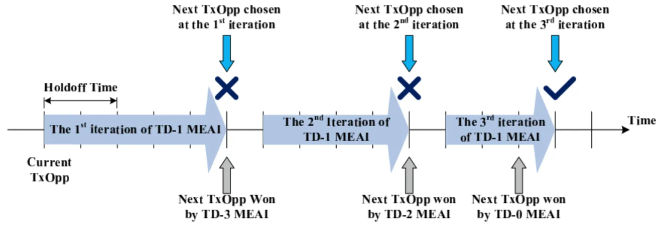
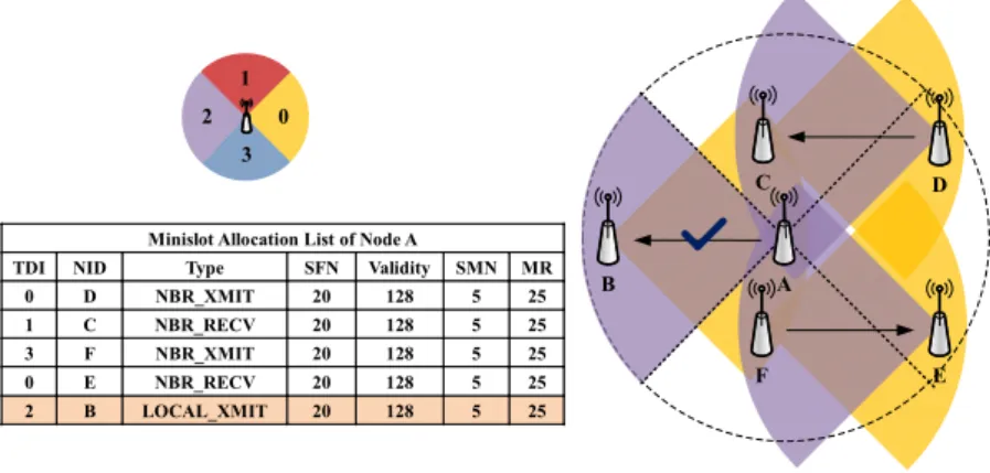
3.14 An example of the iterations of TMEA-D . . . 39 3.15 A minislot scheduling example in a network using omnidirectional antennas 48

(11)

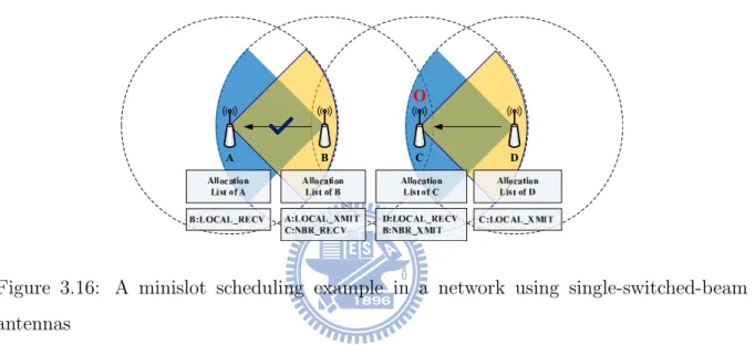
3.16 A minislot scheduling example in a network using single-switched-beam

antennas . . . 48

3.17 An example of data scheduling in a network using single-switched-beam antennas . . . 49

4.1 The transmission cycle of a node . . . 52

4.2 Example case where HR≫ HG . . . 54

4.3 Example case where HR≪ HG . . . 55

4.4 Example case where HR ≫ HG when using the proposed dynamic holdoff time scheme . . . 56

4.5 Comparison between ATHPT values derived from the theoretical model and those obtained by simulations . . . 57

4.6 A good case for establishing a data schedule in the distributed coordinated scheduling mode when the network is not congested . . . 60

4.7 A bad case for establishing a data schedule in the distributed coordinated scheduling mode when the network is not congested . . . 60

4.8 TCP throughputs over different hop counts in chain networks . . . 66

4.9 UDP throughputs over different hop counts in chain networks . . . 66

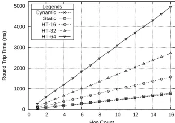
4.10 The round trip time measured by the ping program in chain networks . . . 66

4.11 The operation of the proposed dynamic holdoff time scheme . . . 70

4.12 The topology of the simulated network . . . 74

4.13 The gain pattern of the used single-switched-beam antenna . . . 74

4.14 ATOUN results over different holdoff time exponent values . . . 82

4.15 ATHPT results over different holdoff time exponent values . . . 82

4.16 ATUF results over different holdoff time exponent values . . . 83

4.17 ATTF results over different holdoff time exponent values . . . 83

4.18 ATUF results over different requested frame durations in a THP . . . 84

4.19 ATTF results over different requested frame durations in a THP . . . 84

4.20 ATHPT results over different frame durations under the UDP flow case . . 84

4.21 ATHPT results over different frame durations under the TCP flow case . . 84

4.22 ATUF results over different numbers of requested minislots in a THP . . . 85

4.23 CV-ATUF results over different numbers of requested minislots in a THP . 85 4.24 ATTF results over different numbers of requested minislots in a THP . . . 86

(12)

4.25 CV-ATTF results over different numbers of requested minislots in a THP . 86

4.26 ATOUN results over different numbers of requested minislots in a THP . . 87

4.27 ATHPT results over different numbers of requested minislots in a THP . . 87

4.28 The effects of the fading variance on UDP flow throughputs . . . 91

4.29 The effects of the fading variance on TCP flow throughputs . . . 91

5.1 The procedure of the network entry process . . . 95

5.2 A case in which the network entry process fails . . . 96

5.3 MAC header . . . 99

5.4 The CDF of success rates of network entry processes . . . 102

5.5 The CDF of nodes’ required times for establishing links with all neighboring nodes . . . 102

5.6 Example of MSH-NCFG message collisions . . . 106

5.7 The proposed two-phase holdoff time scheme . . . 108

5.8 Examples of mini-slot allocations scheduled by the basic and MG schemes . 115 5.9 Examples of mini-slot allocations scheduled by the basic and MR schemes . 115 5.10 The protocol stacks of the mesh client, mesh AP, and mesh Internet gate-ways (WMN-to-Internet) . . . 126

5.11 The protocol stacks of the mesh client and mesh AP (WMN-to-WMN) . . 126

5.12 The ARP request and reply procedure in a multi-gateway WMN . . . 131

5.13 The internal protocol stack of a multi-gateway WMN . . . 131

5.14 The simulation topology . . . 133

5.15 The relationship between the number of “short” connections and the total download throughput . . . 136

5.16 The handling of node movement in OSPF . . . 139

5.17 The handling of node movement in STP . . . 139

5.18 The network topology of a two-gateway 5x5 grid WMN . . . 140

6.1 The maximum holdoff exponent values of the four classes proposed in [21] and the transitions among them . . . 145

(13)

List of Tables

2.1 Frequently-used Acronyms . . . 14

3.1 The computation cost of TMEA-S and TMEA-D . . . 38

4.1 The parameter setting used in simulations . . . 63

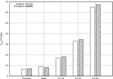
4.2 The performances of the evaluated schemes . . . 64

4.3 MAC-layer performance of the evaluated schemes . . . 69

4.4 The computation cost of the HT-1 scheme and the proposed Dynamic hold-off time scheme . . . 70

4.5 The parameter settings used in the simulations . . . 74

4.6 The used holdoff times of node 1’s TDs . . . 79

4.7 Experienced packet delays of different flows . . . 88

4.8 Throughputs obtained by different flows . . . 88

5.1 Success rates of NENT processes . . . 103

5.2 Average times to establish links with all neighboring nodes for a node . . . 104

5.3 The performances of the four fixed-value holdoff time setting schemes . . . 107

5.4 The parameter setting used in simulations . . . 116

5.5 The performances of the four schemes . . . 117

5.6 The average bandwidth satisfaction index results . . . 118

5.7 The total download throughput in the one-to-multi downlink traffic case . 134 5.8 The number of established and stable connections in the one-to-multi down-link traffic case . . . 134

5.9 Number of established and stable connections with AODV . . . 135

5.10 Relationship between the average hop count and achieved throughput of connections . . . 136

(14)

5.12 The number of established and stable connections in the multi-to-multi peer traffic case . . . 137 5.13 The system total throughput under the mobility condition . . . 138 5.14 The number of established and stable connections under the mobility

con-dition . . . 139 5.15 The system total throughput of a multi-gateway WMN with different

num-ber of gateways . . . 140 5.16 The system total throughput under OSPF and OSPF with ETX in a harsh

wireless environment . . . 141 5.17 The number of established and stable connections under OSPF and OSPF

with ETX in a harsh wireless environment . . . 142 5.18 The total download throughput of single-radio and dual-radio WMNs . . . 142

(15)

Chapter 1 Introduction

The Wireless Mesh Network (WMN) is a cost-effective solution for backbone networks in both metropolitan and rural areas and can be used as temporary broadband access for emergent and tactic purposes. Without the need of wires, WMNs are easy to deploy and reconstruct to satisfy the dynamic needs. The IEEE 802.16 mesh network is a candidate of next-generation WMNs in this decade, which uses a TDMA-based Medium Access Control (MAC) layer and OFDM-based physical layer and mainly operates at a single frequency. In this network, packets can be transferred in a peer-to-peer manner, and network accesses are managed in a TDMA-like fashion.

As shown in Fig. 1.1, network bandwidth is first divided into frames, each of which is subdivided into one control and one data subframes. A control subframe is further divided into Transmission Opportunities (TxOpp) while a data subframe is further divided into minislots. Control messages and data packets are transferred over TxOpps and minislots, respectively.

To avoid conflicts in using TxOpps, the IEEE 802.16 mesh network defines two schedul-ing modes: 1) the Centralized Schedulschedul-ing (CS) mode and 2) Distributed Schedulschedul-ing (DS) modes. In the CS mode, a network is partitioned into tree-based clusters. Each cluster has a Base Station (BS) node responsible for allocating network resources to the Sub-scriber Station (SS) nodes that it services. Although the CS mode provides collision-free transmissions for control messages and data, it has several disadvantages described below. First, the number of routes that can be utilized is unnecessarily reduced. The reason is that the CS mode uses a tree-based topology, which cannot exploit all possible routes in a network, as compared with a mesh-based topology. For the same reason, the only route

(16)

Figure 1.1: The frame structure of the IEEE 802.16 mesh mode

between two nodes on the tree may not be the shortest one between them if instead a mesh-based topology were used. In addition, the root node of the tree is likely to become the performance bottleneck because many packets need to pass through it to reach their destination nodes.

Second, it is difficult to efficiently exploit the spatial reuse property of wireless com-munication in the CS mode. The message format defined in this mode only allows a BS node to notify an SS node of the bandwidth allocated for it. There is no field in the message to allow a BS node to specify the start and end minislot offsets for an allocation. Thus, to avoid interference, each SS node has to take a conservative approach to derive its own data schedule. Allocating minislots in this way is collision-free but results in only one active SS node per cluster at any given time. More detailed explanations about this problem are provided in Appendix.

In contrast, the DS mode provides two advantages. First, the DS mode uses a mesh topology. This allows all possible routing paths to be utilized to avoid performance bottlenecks. Besides, spatial reuse of wireless communication can be exploited to increase network capacity. Second, the DS mode establishes data schedules on an on-demand basis and thus network bandwidth can be more efficiently utilized.

In the IEEE 802.16 mesh network standard, the DS mode is further divided into two operational modes: the coordinated and uncoordinated modes. In the Coordinated Dis-tributed Scheduling (CDS) mode, the control messages required for scheduling minislot allocations are transmitted over TxOpps without collisions. In contrast, in the Uncoordi-nated Distributed Scheduling (UDS) mode, such control messages can only be transmitted on the TxOpps left from the CDS mode or on unallocated minislots. As a result, the CDS mode provides better QoS supports than the UDS mode. In this dissertation, we focus on the 802.16 mesh CDS mode. Fig. 1.2 shows an example IEEE 802.16 mesh CDS-mode network with 25 nodes, where the BS node is at the center of the network.

(17)

al-Figure 1.2: Example of the IEEE 802.16 mesh CDS-mode network

gorithm [1] to resolve contention for TxOpps. Control messages, such as mesh network configuration (MSH-NCFG) and mesh distributed coordinated scheduling (MSH-DSCH) messages, are transmitted on TxOpps determined by this algorithm. (The MSH-NCFG message is used to carry information for network initialization and the MSH-DSCH mes-sage is used to carry information for minislot scheduling.) The contention resolution of MSH-DSCH message transmissions is explained below to illustrate how this pseudo-random algorithm works.

During operation, each node listens to MSH-DSCH messages advertised by its neigh-boring nodes. Based on the scheduling information carried in MSH-DSCH messages, each node knows the transmission interval (shown in Fig. 3.4 and will be explained in detail later) of each of its neighboring nodes. More specifically, it knows for which TxOpps its neighboring nodes may contend. Each node then uses the same election algorithm to determine the winning node for a given TxOpp. This algorithm takes a specified TxOpp number and the IDs of all nodes contending for this TxOpp as input. It outputs the ID of the winning node whose computed value is the largest among all the competing nodes. Conceptually, every node uses the same algorithm and the same input (regarding its own two-hop neighborhood). It thus knows which node will win a given TxOpp within its two-hop neighborhood. As a result, no message collisions will occur on any TxOpp. If a node cannot win a given TxOpp, it repeats the above process with the next TxOpp (i.e., the previous TxOpp number plus one) as input until it eventually wins one TxOpp.

(18)

Figure 1.3: A node’s transmission cycle comprises the holdoff time and the contention time.

After a node wins a TxOpp, the IEEE 802.16 mesh CDS mode requires it to refrain from contending for another TxOpp in a certain number of consecutive TxOpps (called the holdoff time). As shown in Fig. 1.3, a node’s transmission cycle comprises the holdoff time and the contention time. The contention time is defined as the number of consecutive TxOpps in which a node should contend for access (i.e., participate in the algorithm computation) until it wins one. Using this design, every winning node has to suspend its contention for its next MSH-DSCH TxOpp during its holdoff time. Thus, a winning node cannot obtain more than one TxOpp in one transmission cycle, preventing a node from monopolizing a wireless channel. The holdoff time design allows for fair accesses to TxOpps among competing nodes at a cost of increasing delays in transmitting control messages.

The effect of the holdoff time value can be discussed from two aspects. On one hand, if the holdoff time is set to a too large value, network nodes will suffer from long delays in transmitting control messages and thus cannot fully utilize the link bandwidth. In the CDS mode, a network node can transmit data only after it has scheduled a minislot allocation with the intended receiving node. This requires the node and its intended re-ceiving node to perform a Three-way Handshake Procedure (denoted as THP) [1]. THP requires transmitting three MSH-DSCH messages to exchange necessary minislot schedul-ing information, which means that it requires three MSH-DSCH TxOpps to complete the handshake process. Since using a large holdoff time value will increase the transmission cycle for transmitting a control message, the time required for handshaking a minislot allocation (and thus transmitting data) will also be increased.

On the other hand, if the holdoff time is set to a too small value, the number of nodes competing for a TxOpp will be large. This will lead to high contention for TxOpps. In such a congested condition, nodes may experience unpredictable packet delays and share

(19)

TxOpps unfairly. In summary, the holdoff time should be set to an appropriate value that is large enough to avoid congestion but small enough to avoid large transmission delays.

The 802.16 mesh CDS mode uses a fixed holdoff time design in which the holdoff time of each node is a fixed value greater than or equal to 16. This fixed-value design cannot perform optimally for all networks because it does not consider the number of competing nodes and traffic load may vary in the network. To enhance the performances of the 802.16 mesh CDS mode, in this dissertation we propose dynamic holdoff time setting designs for IEEE 802.16 mesh CDS-mode networks using omnidirectional antennas and those using single-switched-beam antennas.

1.1 Problem Description

The IEEE 802.16 mesh CDS mode uses a fixed holdoff time design to schedule the control message transmissions of nodes. This design guarantees the control message trans-missions in the network to be collision-free; however, due to the fixed holdoff time, it is inflexible to adjust nodes’ control message transmissions when network traffic dynami-cally changes. Thus, the IEEE 802.16 mesh CDS mode cannot achieve the most efficient control and data scheduling at all time.

To enhance the performances of this new network, in this dissertation we propose a dynamic holdoff time design that can efficiently schedule the transmissions of control messages and data in the mesh CDS mode network based on dynamic traffic needs. The proposed dynamic holdoff time design can be used in both networks using omnidirectional-antennas and those using directional omnidirectional-antennas. The analytical and numerical results show that our proposed dynamic holdoff time design can significantly enhance the performances of the IEEE 802.16 mesh CDS-mode network.

1.2 Dissertation Organization

The remainder of this dissertation is organized as follows. In Chapter 2, we introduce the operation of the IEEE 802.16(d) mesh CDS mode in detail. In Chapter 3, we explain the proposed dynamic holdoff time designs for IEEE 802.16 mesh CDS-mode networks using omnidirectional antennas and single-beam antennas. In Chapter 4, the performances of the proposed dynamic holdoff time designs are evaluated using both analytical models

(20)

and simulations. In Chapter 5, we discuss the enhancements to the IEEE 802.16 mesh CDS mode in the network initialization process and the minislot handshake process. These enhancements are orthogonal to our main work; however, they significantly affect the performances of this network. We then present related work in Chapter 6. We finally conclude this dissertation and present our future work in Chapter 7.

(21)

Chapter 2 Introduction to the IEEE 802.16(d)

Mesh CDS Mode

In the IEEE 802.16(d) Mesh CDS-mode network, link bandwidth is divided into frames on the time axis and managed in a time-division-multiple-access (TDMA) manner. Each frame comprises one control and one data subframes. A control subframe is further divided into TxOpps, whereas a data subframe is further divided into minislots. Control messages and data packets are transmitted over TxOpps and minislots, respectively.

The 802.16 mesh CDS mode defines three types of control messages: 1) Mesh Net-work Entry (MSH-NENT); 2) Mesh NetNet-work Configuration (MSH-NCFG); and 3) Mesh Distributed Coordinated Scheduling (MSH-DSCH). The MSH-NENT and MSH-NCFG messages are used for nodes to exchange control information for network initialization whereas the MSH-DSCH message is used for nodes to schedule minislot allocations. A minislot allocation is a set of consecutive minislots across several consecutive data sub-frames for data packet transfers. The mesh CDS-mode standard categorizes TxOpps into three types, each for transmitting a specific type of control messages. The TxOpps used for transmitting MSH-NENT messages are called MSH-NENT TxOpps; those used for transmitting MSH-NCFG messages are called MSH-NCFG TxOpps; and those used for transmitting MSH-DSCH messages are called MSH-DSCH TxOpps. The detailed usages of these TxOpps are defined in [1].

(22)

Figure 2.1: The procedure of the network entry process

2.1 Network Initialization

To join an IEEE 802.16(d) mesh network, an SS must perform the “network entry” process to attach itself to the network. An SS cannot transmit and receive data packets until it finishes its network entry process. As shown in Fig. 2.1, in the network entry process a new SS first monitors the MSH-NCFG messages broadcast from its neighboring operational nodes. (A operational node is an SS that has completed its network entry process.) Based on the received MSH-NCFG messages, this new node builds a neighboring node list that records the ID and operational information of its neighboring operational nodes.

With this list, the new node can start attaching itself to the network. It first selects one of its neighboring operational nodes as its sponsoring node. Then it transmits a network entry request (NetEntryRequest) information element (IE), which is carried in an MSH-NENT message, to the chosen sponsoring node. Upon receiving such a message, the sponsoring node determines whether it can (and is willing to) service this new node. If not, it ignores this message. Otherwise, it reserves a temporary minislot allocation for the new node and then responds the new node with an MSH-NCFG message that carries an EntryOpenIE.

When receiving the MSH-NCFG:EntryOpenIE message, the new node first acknowl-edges its sponsoring node with a NetEntryAckIE (which is carried in an MSH-NENT

(23)

message) and then performs the capability negotiation, authorization, and registration procedures with a BS node in the network using the minislot allocation temporarily re-served by the sponsoring node for it. After finishing the registration procedure, the new node has attached itself to the network.

The next step is to transmit a NetEntryCloseIE (which is carried in an MSH-NENT message) to its sponsoring node. The NetEntryCloseIE is used to notify the sponsoring node that the new node has joined the network and thus the temporary minislot alloca-tion is no longer required. Upon receiving this message, the sponsoring node cancels the temporary minislot allocation reserved for the new node and replies the new node with a NetEntryAckIE (which is carried in an MSH-NCFG message), to terminate this sponsor-ship. Upon receiving the MSH-NCFG:NetEntryAckIE message, the new node finishes its network entry process and becomes a operational node in the network.

2.2 Control Message Scheduling

In the 802.16 mesh CDS mode, each node’s control message transmission is sched-uled by the Mesh Election Algorithm (MEA) [1], which is hash-based algorithm with an exponential holdoff mechanism. In this mode, each node needs to maintain (i.e., learn) the information about its hop neighborhood (which is an input of MEA). The two-hop neighborhood of a node is defined as the set comprising the node itself, its one-two-hop neighboring nodes, and its two-hop neighboring nodes, i.e.,

nbr(i) = {i} ∪ nbr1(i) ∪ nbr2(i), (2.1)

where nbr1(i) and nbr2(i) are defined as follows, respectively.

nbr1(i) = {k | node k ∈ node i’s one-hop neighboring nodes,

when omnidirectional antennas are used.} (2.2)

nbr2(i) = {k | node k ∈ node i’s two-hop neighboring nodes,

when omni-directional antennas are used.} (2.3)

The purpose of maintaining the two-hop neighborhood is to avoid the hidden terminal problem when transmitting control messages. By using the same MEA in every node, this algorithm guarantees that in the network only one node in any two-hop neighborhood will

(24)

win the access to a specific TxOpp. Thus, when nodes transmit their control messages, no message collisions will occur. Since the transmission of control messages are collision-free and these messages are used for scheduling a collision-collision-free minislot allocation, the transmission of data can also be guaranteed collision-free.

The scheduling process of the MSH-DSCH message in the 802.16 mesh CDS-mode

network is explained here1_{. Each node should perform MEA to determine the TxOpp on}

which to broadcast its next MSH-DSCH message. MEA takes a given TxOpp number and an eligible node list (which is a list of nodes that are eligible to contend for the given TxOpp) as input. It then iteratively computes a hash value for each node in the given eligible node list on the give TxOpp number. The hash function is given in [1]. Finally, it outputs the ID of the winning node whose computed hash value i s the largest among all of the competing nodes. Because nodes within two hops use the same MEA and consistent eligible node lists, every node knows which node will win a given TxOpp within its two-hop neighborhood.

To achieve the consistency of neighboring nodes’ eligible node lists for each TxOpp, each node should periodically broadcast the next MSH-DSCH TxOpps used by itself and its one-hop neighboring nodes. In addition, for node i, if the information about the next MSH-DSCH message transmission of its neighboring node j is unknown, node i will conservatively consider that node j will contend for every TxOpp and put node j into the eligible node list for the following TxOpps until it receives the information about the next MSH-DSCH TxOpp used by node j. Using this design, no message collision will occur on any TxOpp. If a node cannot win a given TxOpp, it repeats the above process with the next TxOpp (i.e., the previous TxOpp number plus one) as input until it eventually wins one TxOpp.

The eligibility of a node for contending for a TxOpp is determined by the holdoff time mechanism [1]. The holdoff time mechanism first defines the control message transmission cycle of a node as the time interval between the node’s two consecutive control message transmissions. Recall that, as shown in Fig. 2.2, the transmission cycle of a node comprises 1) the holdoff time and 2) the contention time. The former is defined as the number of consecutive TxOpps during which a node must suspend its contention for TxOpps after

1_{The scheduling process of the MSH-NCFG message is the same as that of the MSH-DSCH message.}

(25)

Figure 2.2: The transmission cycle of a node

wining a TxOpp, while the latter is defined as the number of consecutive TxOpps for which a node may contend to win a TxOpp. Thus, by obtaining the holdoff times of the nodes in its two-hop neighborhood, a node can know for which TxOpps these neighboring nodes will and will not contend. Based on such information, it can construct an eligible node list of its two-hop neighborhood for every TxOpp.

In the 802.16(d) mesh CDS mode, the holdoff time of each node is fixed and defined as follows:

HT(i) = 2exp+base, (2.4)

where HT(i) denotes the holdoff time of node i. The base value is fixed to 4 and the range of the exp value is between 0 and 7. In the 802.16 mesh mode standard, the exp value of each node is the same. Thus, the holdoff times of all nodes in the network are the same. In contrast, the contention times of nodes may vary depending on which and how many nodes are eligible to contend for TxOpps.

Before broadcasting an MSH-DSCH message, a node first executes MEA to calculate (win) a TxOpp for its next MSH-DSCH message transmission. It then puts the following information into the MSH-DSCH message that is going to be sent out: 1) its calculated next MSH-DSCH TxOpp number; 2) its holdoff time; 3) the learned next MSH-DSCH TxOpp numbers of its hop neighboring nodes; and 4) the holdoff times of these one-hop neighboring nodes. After this, it broadcasts this MSH-DSCH message to all of its neighboring nodes.

By this design, a node can learn in advance the next MSH-DSCH TxOpp numbers and holdoff times of all nodes in its two-hop neighborhood. Because every node knows such information about every other node in its two-hop neighborhood, for any given TxOpp, the output of every node’s MEA in any two-hop neighborhood is consistent. The consistency of the MEA output means that: For nodes i and j, suppose that {a, b} = nbr(i) ∩ nbr(j),

(26)

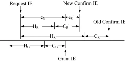
Figure 2.3: The THP defined in the IEEE 802.16(d) mesh CDS mode

it is impossible that a and b simultaneously win the same TxOpp. That is, in a two-hop neighborhood, there is only one winning node for a given TxOpp and every node knows who wins it. As a result, when nodes transmit their MSH-DSCH messages, no collision will occur. It is this advance announcement design that enables MEA to generate collision-free control message scheduling.

Another advantage of the holdoff time design used in the 802.16 mesh CDS mode is that, using this design, a node must refrain from contending for TxOpps after winning a TxOpp (i.e., after transmitting its current MSH-DSCH message) until its holdoff time has elapsed. This ensures that nodes other than the winning node will have a chance to win subsequent TxOpps and all nodes can fairly share TxOpps in the long run.

2.3 Data Minislot Scheduling

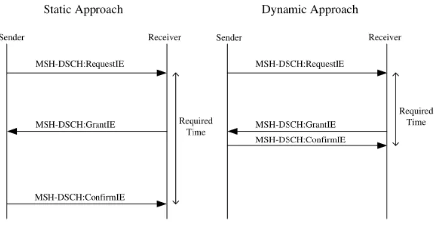
The IEEE 802.16(d) mesh CDS mode schedules data transmissions of nodes in a distributed and on-demand manner. A three-way handshake procedure (THP) [1] is used for a pair of nodes to negotiate a minislot allocation agreed by both nodes. A minislot allocation is a set of consecutive minislots on which the transmitting node and the receiving node are sure that they are ready to transmit and receive data packets. As shown in Fig. 2.3, THP uses a “request-grant-confirm” control sequence for two peer nodes to negotiate a minislot allocation. In a THP, the requesting node first transmits a request IE and an availability IE to the granting node using an MSH-DSCH message. The request IE specifies the number of minislots that the requesting node needs to transmit data packets and the availability IE specifies a set of consecutive minislots on which the requesting node can transmit data packets.

(27)

On receiving a request IE, the granting node first determines whether it can receive data packets from the requesting node within the minislot set specified by the received availability IE. If not, the granting node can simply ignore the received request IE. Other-wise, it allocates a minislot allocation within the specified minislot set and then transmits a grant IE to the requesting node as an acknowledgment using its MSH-DSCH message. The grant IE specifies a subset of the minislots specified by the received availability IE on which the granting node is willing to receive data packets from the requesting node. Upon receiving the grant IE, the requesting node then broadcasts a confirm IE using its MSH-DSCH message to complete this THP. The confirm IE is a copy of the received grant IE and used to notify the requesting node’s one-hop neighboring nodes of the duration on which this minislot allocation will take place.

2.4 Acronym Table

Many acronyms are used in this dissertation to make it concise. To help readers easily refer to the meanings of these acronyms, frequently-used acronyms are collected and defined in Tab. 2.1.

(28)

Table 2.1: Frequently-used Acronyms

Acronym Meaning

ATUF Average Throughput of a UDP Flow in a network

ATTF Average Throughput of a TCP Flow in a network

ATHPT Average Three-way Handshake Procedure Time

ATOUN Average Transmission Opportunity Utilization of Nodes

BS Base Station

CDS Coordinated Distributed Scheduling

CS Centralized Scheduling

CV-ATUF The Coefficients of Variation of all nodes’ ATUF values

CV-ATTF The Coefficients of Variation of all nodes’ ATTF values

MEA Mesh Election Algorithm

MEAI Mesh Election Algorithm Instance

TMEA-S Transmission-domain-aware Mesh Election Algorithm with a Static holdoff time design

TMEA-D Transmission-domain-aware Mesh Election Algorithm with a Dynamic holdoff time design

MSH-DSCH Mesh Distributed Scheduling

MSH-NCFG Mesh Network Configuration

MSH-NENT Mesh Network Entry

MTD Multi-transmission-domain

NetUI Network Unfairness Index

NodeUI Node Unfairness Index

STD Single-transmission-domain

TD Transmission Domain

TDI Transmission Domain Index

THP Three-way Handshake Procedure

TMEA Transmission-domain-aware Mesh Election Algorithm

TMSA Transmission-domain-aware Minislot Scheduling Algorithm

TxOpp Transmission Opportunity

(29)

Chapter 3 Proposed Dynamic Holdoff Time

Designs

3.1 Proposed Scheme for Networks using Omni-directional

Antennas

3.1.1 Motivation

In Section 1, we have explained that the IEEE 802.16 mesh CDS mode uses a fixed holdoff time design to schedule the control message transmissions of nodes. Due to this fixed holdoff time, it is inflexible to adjust nodes’ control message transmissions when network traffic dynamically changes. Thus, the IEEE 802.16 mesh CDS mode cannot achieve the most efficient control and data scheduling at all time.

One intuitive alternative is to totally shutdown the control message transmissions of those nodes that do not have data to send. However, as explained in Section 2.2, if a node does not transmit its control messages (i.e., MSH-NCFG and MSH-DSCH messages), based on [1] its neighboring nodes will conservatively consider that this node will contend for every TxOpp. In this condition, the number of contending nodes per TxOpp will be increased (due to the unknown status of the node that disables its control message transmissions).

To solve this problem, the formats of the MSH-NCFG and MSH-DSCH messages should be expanded to allow a node to use a very large holdoff time value (or the infi-nite holdoff time value). Using such a design, when a node disables its control message

(30)

Sender Receiver MSH-DSCH:RequestIE MSH-DSCH:GrantIE MSH-DSCH:ConfirmIE Required Time Receiver MSH-DSCH:RequestIE MSH-DSCH:GrantIE MSH-DSCH:ConfirmIE Required Time Sender

Static Approach Dynamic Approach

Figure 3.1: The advantage of the proposed dynamic holdoff time scheme

transmissions for a very long period, its neighboring nodes can safely exclude it from the contending node lists of subsequent TxOpps, which can effectively reduce the number of contending nodes per TxOpp. Because this solution requires the expansion of control message formats, we do not adopt this solution to avoid changing the message formats of the IEEE 802.16 mesh CDS-mode specification.

3.1.2 Design

The main idea of the proposed dynamic holdoff time scheme is to decrease the trans-mission cycles of nodes, when they have data to send. This is accomplished by decreasing the time required by nodes to complete their THPs. By doing this, per-hop (and end-to-end) data transmission delays can be decreased and per-hop (and end-end-to-end) data transmission throughputs can be increased.

Using the proposed dynamic holdoff time scheme, a requesting node can reduce the time interval between transmitting its request IE and transmitting its confirm IE. That is, using this scheme, on receiving a grant IE from the granting node, a requesting node will transmit a confirm IE as soon as possible. As shown in Fig. 3.1, the proposed dynamic holdoff time scheme can on average save about a half of the time required to establish a minislot allocation, compared with fixed holdoff time schemes.

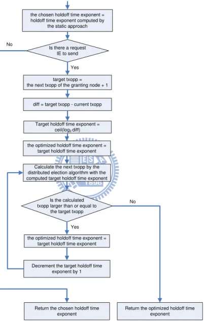
The detailed algorithm of our proposed dynamic holdoff time scheme is shown in Fig. 3.2 and explained here. In this scheme, the holdoff time base value is set and fixed to 0 rather than the default 4. Initially, a node using the proposed scheme determines its

(31)

holdoff time using the following formula:

HT(i) = 2f loor(log2(|nbr(i)|)) _(3.1)

where nbr(i) is the number of nodes in node i’s two-hop neighborhood and defined in Eq. (2.1). If this node does not have data to send,it regularly transmits its MSH-DSCH messages using Eq. (3.1) to keep MEA operating correctly. Note that even though there is no data to send, a node still needs to send out its MSH-DSCH messages regularly to maintain the operation of its MEA. The transmitted MSH-DSCH messages are used to notify this node’s neighboring nodes of its next MSH-DSCH message transmission time. These MSH-DSCH messages, however, need not carry minislot scheduling information, such as request, grant, and confirm IEs.

In contrast, when a node has data to send, it first needs to launch a THP (i.e., transmit a request IE out). In this condition, before the requesting node transmits out the request IE, it calculates the earliest TxOpp where it can transmit the confirm IE to the granting node in advance. Note that transmitting the confirm IE must be performed later than receiving a grant IE from the granting node. To ensure this sequence, the requesting node’s target TxOpp (i.e., the next TxOpp used to transmit the confirm IE) is initially set to the next TxOpp of the granting node plus one. Note that the requesting node knows this information because this information is regularly exchanged among nodes via the MSH-DSCH messages.

Then, it uses the difference between its current and the target TxOpps to calculate the maximum target holdoff exponent value as follows:

max target holdoff exp = ⌈log2(difference)⌉ (3.2)

This calculated exponent value is used as the initial exponent value to find a TxOpp that is later than the target TxOpp. The found TxOpp is the output of MEA and will be larger than the target TxOpp due to the existence of the contention time.

Later on, our proposed dynamic holdoff time scheme then goes through an iteration to find the smallest exponent value that makes the transmission of the confirm IE as close as possible to the reception of the granting IE. During each step of the iteration, the target holdoff time exponent is decremented by one to explore whether this smaller value can still meet the requirement. On the last step of the iteration, where the requirement can no longer be met, the exponent value used in the previous step (which is stored in the

(32)

Is there a request IE to send

target txopp = the next txopp of the granting node + 1

diff = target txopp - current txopp Target holdoff time exponent =

ceil(log2diff)

Calculate the next txopp by the distributed election algorithm with the computed target holdoff time exponent

Is the calculated txopp larger than or equal to

the target txopp

Return the chosen holdoff time exponent

Yes

No Yes

No

the chosen holdoff time exponent = holdoff time exponent computed by

the static approach

Decrement the target holdoff time exponent by 1

the optimized holdoff time exponent = target holdoff time exponent

Return the optimized holdoff time exponent

(33)

optimized holdoff time exponent variable) is the exponent value that is both feasible and the smallest. This value is then returned and used to derive the TxOpp for transmitting the confirm IE.

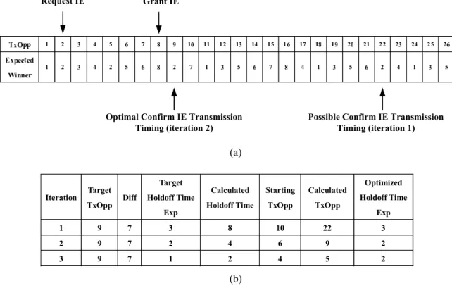
Fig. 3.3 shows an example illustrating the operation of the proposed dynamic holdoff time scheme. Suppose that the two-hop neighborhood of node 2 comprises eight nodes, including node 2 itself. Fig. 3.3(a) shows the winning nodes of the TxOpps numbered from 1 to 26. Here, the winning node of a TxOpp is defined as the node that wins this TxOpp when all of the eight nodes contend for this TxOpp. (This condition will occur if the holdoff time base value is set to zero. The effect of the holdoff time base value will be explained in detail in Section 3.1.3.) Assume that node 2 intends to schedule a minislot allocation with node 8. Before transmitting the request IE to node 8 on TxOpp 2, node 2 should perform the algorithm depicted in Fig. 3.2. The detailed steps executed by this algorithm are explained below.

As shown in Fig. 3.3(b), the proposed algorithm first sets the target TxOpp to 9, which is right after the TxOpp that node 8 is likely to transmit its grant IE (assuming 8 in this example). The algorithm calculates the TxOpp that node 2 can win. During the first iteration, the algorithm first finds that node 2 can win TxOpp 22. Since the calculated transmission opportunity (22) is still larger than the target TxOpp, the algorithm stores the current target holdoff time exponent value into the optimized holdoff time exponent variable, decrements the target holdoff time exponent value by one, and starts the second iteration. During the second iteration, it finds that node 2 can win TxOpp 9. However, because the calculated TxOpp (9) is still larger than or equal to the target TxOpp, it enters the third iteration to probe further optimization.

During the third iteration, the algorithm finds that the calculated TxOpp is 5, which now is less than the target transmission opportunity. Thus, it stops this iterative pro-cedure and returns the value stored in the optimized holdoff time exponent variable as its output. (Note: This value is the target holdoff time exponent value calculated in the previous iteration.) As can be seen in Fig. 3.3(b), upon performing the MEA with the optimized holdoff time exponent value (2 in this example), node 2 will win TxOpp 9, which is the optimal transmission timing to transmit its confirm IE in this example.

(34)

Figure 3.3: An example illustrating the operation of the dynamic approach

3.1.3 Effect of Holdoff Time Base Value

As introduced earlier, the IEEE 802.16 mesh CDS mode regulates that every node should set the holdoff time base value to 4. With this regulation, radios compliant to the 802.16 mesh CDS mode co-cooperate using this fixed holdoff time base value. Our proposed dynamic holdoff time scheme, however, may require changing the holdoff time base value to operate. For this reason, a mechanism is required to notify network nodes of changes to the holdoff time base value. In this section, we explain the problems that may occur if this system parameter is dynamically changed. In Section 3.1.4, we will describe several mechanisms that can be used to change this parameter without causing problems.

The holdoff time base value contributes a constant time amount (2base_{) to the holdoff}

time. Setting the holdoff time base value to 4 means that each node should suspend its

contention for at least 24 _{consecutive TxOpps after it has won one. This lower bound}

limits the smallest holdoff time value that can be assigned to nodes in the proposed dynamic holdoff time scheme. The proposed dynamic holdoff time scheme, therefore, cannot achieve its optimal performances, if the holdoff time base value is not reduced to 0. For this reason, in our proposed dynamic holdoff time scheme the holdoff time base value of the network is set to zero to provided the largest flexibility of control message

(35)

scheduling.

Instead of using a lengthy field, the standard uses two shorter fixed-length fields, exp and Mx, to represent a TxOpp number. The relationship between these two fields and a TxOpp number has been given as follows:

2exp ∗ Mx < next TxOpp <= 2exp ∗ (Mx + 1), (3.3)

where next TxOpp denotes a node’s next TxOpp number.

On receiving a control message (such as an MSH-NCFG message or an MSH-DSCH message), a node should use the received exp and Mx fields to derive the next transmission interval of the transmitting node using Eq. (3.3). Fig. 3.4 shows the relationship between the holdoff time and the transmission interval (Tx Interval). The holdoff time comprises the Tx interval (denoted as α in the figure) and the ineligible interval (denoted as β in the figure). The Tx interval represents the duration in which a node may contend for one TxOpp. On the other hand, the ineligible interval is the duration in which the node is not allowed to contend for any TxOpp.

Based on Eq. (3.3), the length of the Tx interval is fixed to 2exp _{because a node’s}

next TxOpp number is within a fixed-length interval ranging from (2exp_{∗ Mx + 1) to}

2exp_{∗ (Mx + 1). Consequently, the length of the ineligible interval is (2}exp+base _{- 2}exp_{). If}

the base value is set to 0, the holdoff time and the Tx interval of each node will exactly overlap, causing the length of the ineligible interval to be zero. This means that, after winning a TxOpp, a node will contend for another TxOpp immediately. (This also means that a node will contend for TxOpps all the time.) Thus, a node should consider that all nodes in its two-hop neighborhood will contend for each TxOpp with itself. On the other hand, if the holdoff time base value is larger than 0, a node’s holdoff time will be larger than its Tx interval. In this condition, the contention time experienced by a node can be reduced due to a decreased number of contending nodes.

The choice of the holdoff time base value depends on the needs of a holdoff time scheme. For a static holdoff time scheme, using a positive holdoff time base value can reduce the contention time of each node. For a dynamic holdoff time scheme, however, the holdoff time base value must be zero for two reasons: First, if a positive holdoff time base value is used, the lower bound of the holdoff time value that can be assigned to nodes will be limited. Thus, to give the dynamic holdoff time scheme the largest freedom to set nodes’ holdoff times, the holdoff time base value should preferably be set to zero at all

(36)

exp+base

exp

exp exp

Figure 3.4: The relationship between the holdoff time and the Tx interval

time. Second, if the holdoff time base value is allowed to change during the operation of a network, after a node’s holdoff time has just been changed (due to the change of the holdoff time base value), MSH-DSCH control messages may collide. The reason for this phenomenon is explained below.

Fig. 3.5 and Fig. 3.6 show two cases after a node’s holdoff time value has just been changed. The former shows an example that changing the holdoff time value results in no message collisions while the latter shows an opposite example. Suppose that node A has changed its holdoff time value and broadcast the new holdoff time exponent value. In Fig. 3.5, node B is the next one to transmit an MSH-DSCH message. In this case, node C will be notified of this change by node B’s MSH-DSCH message in time. Thus, node C will not schedule its MSH-DSCH message transmission to collide with node A’s MSH-DSCH message transmission.

In contrast, in Fig. 3.6 node C has scheduled an MSH-DSCH message transmission before node B can notify it of node A’s new holdoff time value. In this condition, node C’s MSH-DSCH message transmission may collide with node A’s MSH-DSCH message transmission because node A’s ineligible interval viewed by node C now becomes out of date. Figures 3.7, 3.8, and 3.9 illustrate three cases that can cause this problem.

In these figures, HTa denotes the holdoff time of node A viewed by node C (may be

out of date) and HTa′ _{denotes the holdoff time of node A viewed by node A itself (always}

up to date). The symbol γ denotes the vulnerable interval that results from node A’s changing its holdoff time and during which the MSH-DSCH messages of nodes A and C may collide. Suppose that node C’s transmission was scheduled within node A’s original ineligible interval β. Fig. 3.7 depicts a case that node A has just decreased its holdoff

time base value and therefore its ineligible interval is just shortened from β to β′_{. This}

(37)

A B C

1 2

Figure 3.5: An example showing that control messages will not collide after node A changes its holdoff time value

A B C

1 2

Figure 3.6: An example showing that control messages will collide after node A changes its holdoff time value

(38)

Node C HTa ȕ Į Node A HTa' ȕ' Į Ȗ

Figure 3.7: A case that node A has just decreased its holdoff time base value

Node C HTa ȕ Į Node A HTa' ȕ' Į' Ȗ

Figure 3.8: A case that node A has just increased its holdoff time exponent value now will contend for TxOpps in the γ interval.

Fig. 3.8 depicts a case that node A has just increased its holdoff time exponent value and therefore both its Tx Interval and ineligible interval are lengthened. In this condition, node A’s ineligible interval will shift on the time axis, generating the vulnerable interval shown in Fig. 3.8. In contrast, Fig. 3.9 depicts a case that node A has just decreased its holdoff time exponent value and therefore its Tx Interval and ineligible interval are shortened, resulting in the shift of node A’s ineligible interval on the time axis. This shift generates the vulnerable interval shown in Fig. 3.9.

To prevent the collision problem from occurring, an additional mechanism to advertise nodes’ changes to their holdoff time base and exponent values in time is needed. For instance, in the case given in Fig. 3.6, after changing the holdoff time value, node A should defer its contention for TxOpps until its original ineligible interval has elapsed. Such a mechanism, however, may increase the implementation complexity of a proposed

Node C HTa ȕ Į Node A HTa' ȕ' Į' Ȗ

(39)

dynamic holdoff time scheme and decrease its scheduling performances. To totally avoid the collision problem without wasting much network bandwidth, our proposed dynamic holdoff time scheme uses 0 as the holdoff time base value for all network nodes at all time. Fixing the holdoff time base value to zero effectively eliminates every node’s ineligible interval (i.e., the length of each node’s ineligible interval now becomes zero.), resulting in each network node considering that it should always contend for TxOpps with all other nodes in its two-hop neighborhood. (These two-hop neighborhood nodes are considered to be always eligible to contend for TxOpps.) In this condition, if a node intends to win a TxOpp, it should win over all of its two-hop neighborhood nodes. This means that, for each node, the node list used as the input of MEA will always comprise its two-hop neighborhood nodes, despite the dynamic changes of the holdoff time exponent values of its neighboring nodes. Thus, packet collisions due to dynamic changes of the holdoff time exponent values can be avoided under the zero holdoff time base value condition.

3.1.4 Notification of Holdoff Time Base Value Change

Here, we propose a practical protocol that can notify new SS nodes of the holdoff time base value used in a network. A BS node can use this protocol to check whether a new SS node can operate using a holdoff time base value other than 4. If an SS node cannot do so, the BS node should reject the network registration request from this SS node because this SS node cannot work well with other SS nodes in the network.

Our proposed protocol exploits the reserved “vendor-specific information” field to help SS nodes know the holdoff time base value used in the network. This field is defined in the standard for the registration procedure to exchange additional information not specified in the standard. The signaling protocol is described as follows: An SS node first adds a holdoff time base query message (carried by the “vendor-specific information” field) into the registration request (REG-REQ) message, which is destined to the BS node.

On receiving this REG-REQ message, the BS node replies the SS node with a regis-tration response (REG-RSP) message, which contains the holdoff time base value used in this network (also carried by the “vendor-specific information” field). If the BS node does not find the holdoff time base query message in the SS node’s REG-REQ message, it should reject this SS node’s registration request because this SS node may not be able to change its holdoff time base value.

(40)

There are three ways to reject a registration request. The first one is simply to ignore the REG-REQ message if the BS node decides to reject it. The second way is to utilize the “de/re-register command” (DREG-CMD) message, defined in the standard. The DREG-CMD message can be used to notify the SS node of the rejection action. The last way is to return a REG-RSP message with the response code set to 1, indicating that this registration request cannot be accepted because the SS node may not be capable of changing its holdoff time base value.

3.2 Proposed Scheme for Networks using

Single-switched-beam Antennas

The effects of MEA on the performances of the 802.16(d) mesh CDS mode have been extensively studied [2][3][4][5][6]; however, most of the prior work were based on omni-directional radios. In the literature, rare work studied the performances and challenges of the 802.16(d) mesh CDS-mode network when it uses directional antennas. Because the 802.16(d) mesh CDS mode assumes that MEA operates using omnidirectional radios, MEA encounters several operational problems when operating over directional radios.

Recent antenna technologies for directional message transmission/reception can be categorized into three classes. The first class is the switched-beam antenna, which uses pre-defined antenna gain patterns and can point to several pre-determined directions. Switched-beam antennas can operate optimally in environments without the presence of the multi-path effect (such as in the free-space environment). Due to lacking the nulling capability, however, they cannot achieve the optimal concurrent transmission schedules in multi-path-prone environments, as compared with the other two directional antenna classes.

The second antenna class is the adaptive array antenna, which is capable of forming arbitrary beams to point to arbitrary directions. By forming “nulls” to directions in which a transmitter does not intend to disseminate its signal or from which a receiver does not intend to sense the signal, adaptive array antennas can effectively reduce the multi-path effects. The last antenna class is the Multiple Input Multiple Output (MIMO) array antenna, which employs multiple antenna elements on both the transmitter and receiver ends. MIMO is well-known for its three capabilities: precoding, spatial multiplexing, and

(41)

diversity coding, which can more effectively increase network capacity.

Although adaptive array antennas and MIMO antennas can be superior to switched-beam antennas in achieved network capacity and signal quality, the cost and complexity of their designs and implementations are much higher than those of switched-beam an-tennas. Due to the less design and implementation complexity, switched-beam antennas can be made with less form factor and at a lower cost; they therefore provide a cost-effective solution for wireless mesh networks using directional radios and more suitable for constructing emergent and tactic wireless mesh networks.

In this section, we reviewed the design of the 802.16 mesh CDS mode, identified the problems that result from using single-switched-beam antennas in this network, and proposed a scheme to solve these problems. The proposed scheme can operate using only directional transmissions/receptions. (Most of the previous proposals for directional antenna networks have to use omnidirectional transmissions/receptions in some phases of network operation.) We conducted proof-of-concept simulations to evaluate the network capacity increased by using single-switched-beam antennas in this network. In addition, we also evaluated the performances of TCP (Transport-layer Control Protocol) using a real-life TCP implementation in such networks. TCP is a well-known transport-layer protocol widely used in current network applications (such as FTP, HTTP, etc.) and is sensitive to network congestion and end-to-end packet delay jitters. Due to the unique protocol design of the 802.16 mesh CDS mode, how TCP performs under this network with single-switched-beam antennas is interesting and worth studying.

To the best of the authors’ knowledge, our work is the first work that discusses how to enable the IEEE 802.16(d) mesh CDS-mode network to operate with single-switched-beam antennas and evaluates the performances of this network with single-switched-single-switched-beam antennas. Although there have been many prior works studying TDMA networks with di-rectional radios [7][8][9][10][11][12][13][14][15][16][17], they differ from the IEEE 802.16(d) mesh CDS mode using single-switched-beam antennas in either control message scheduling or data scheduling. Thus, the issues and performances of the IEEE 802.16(d) mesh CDS mode employing such an antenna configuration is worth studying. Although the IEEE 802.16 mesh mode may not be maintained in the next-generation 802.16 standard family due to several reasons, e.g., its design complexity is higher than that of the traditional point-to-multipoint (PMP) mode and its current business potential is less than that of the

(42)

PMP mode, in the literature so far it is one of the most representative WMNs that have been well developed and studied and can be a good design reference for next-generation WMNs.

In this dissertation, we do not assume that a single-switched-beam antenna allows omnidirectional transmission and reception because the antenna gain of such an antenna in the directional mode and that in the omnidirectional mode may greatly vary. Without proper transmission power control, the connectivity among nodes in the directional mode and that in the omnidirectional mode may be inconsistent and hinder network operation. To simplify the scheduling complexity, our proposed scheme operates only with pure directional transmission and reception. As a result, several protocol issues will arise due to such a harsh constraint. For example, in the IEEE 802.16(d) mesh CDS mode each node maintains its two-hop neighborhood to avoid the hidden-terminal problem when transmitting its control messages. The definition of such a two-hop neighborhood is based on the use of omnidirectional antennas and thus has an important property: if

node A is in node B’s two-hop neighborhood, then node B is also in node A’s two-hop neighborhood. It is this property ensuring that the MEA used in each node generates

collision-free TxOpp scheduling because node A and node B cannot both win the same TxOpp in their respective two-hop neighborhoods. However, when only pure directional transmission and reception are allowed (e.g., when using single-switched-beam antennas), the above property no longer holds at all time. This makes receiving control messages from other nodes non-trivial. In this condition, network operation and network initialization encounter several issues that need to be solved. In the following, we explain the problems of the IEEE 802.16(d) mesh CDS mode, when it uses single-switched-beam antennas to operate and initialize the network, and present our solutions to these problems.

3.2.1 Problem 1: Imprecise Representation for TxOpps in

Con-trol Messages

In the 802.16(d) mesh CDS mode, to save the bandwidth consumed by control mes-sages, the next TxOpp number of a node carried in an MSH-DSCH message and an MSH-NCFG message is represented by a 5-bit Mx field and a 3-bit Exp field [1], rather than a single long field. Using this representation scheme, a TxOpp number is represented

(43)

using the following formula:

2exp_{∗ Mx < TxOpp number ≤ 2}exp_{∗ (Mx + 1),} _(3.4)

where 0 ≤ Mx ≤ 30, 0 ≤ exp ≤ 7. The interval between (2exp_{∗ Mx, 2}exp_{∗ (Mx+1)] is}

called the next transmission interval of a control message in the standard.

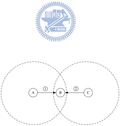
It is known that using MEA no two nodes in the same two-hop neighborhood will use the same TxOpp to transmit messages. However, the transmission intervals of two nodes in the same two-hop neighborhood may overlay with each other. For example, consider two nodes A and B are in node C’s two-hop neighborhood. Suppose that the current TxOpp is 0 and nodes A and B choose TxOpps 33 and 36 as their next MSH-DSCH

TxOpps, respectively. In this condition, both nodes A and B may use (25 _{∗ 1, 2}5 _{∗ 2]}

(base=4, exp=1, Mx=1) as their next transmission intervals and notify node C of these settings.

The overlapping of two neighboring nodes’ transmission intervals does not hinder the operation of the 802.16(d) mesh CDS mode, when omnidirectional radios are used, because each node can listen incoming messages omnidirectionally, when it need not transmit control messages. In this condition, a node will not miss any control messages broadcast from neighboring nodes as long as it is not in the transmission state. However, when only directional reception is allowed, a node cannot determine to which direction its antenna should point because this imprecise representation cannot provide sufficient information for a node to know which node will transmit a message on a specific TxOpp among those nodes whose next transmission intervals are overlapped.

In addition, even though the transmission intervals of neighboring nodes do not over-lap with each other, this imprecise representation scheme still reduces the flexibility of scheduling control message transmissions. Consider nodes A and B that are neighboring to each other. Using this TxOpp representation scheme, on receiving an MSH-DSCH message from node B, node A cannot know the exact next TxOpp number won by node

B. Instead, it can only derive an interval of 2exp _{TxOpps in length during which node}

B will broadcast its next MSH-DSCH message. Since node A cannot know the exact next TxOpp that node B wins, it has to point its antenna towards node B during the whole interval to successfully receive the next MSH-DSCH message broadcast from node B. However, if the exact next TxOpp won by node B can be known, node A can exchange control messages with some other nodes in this long interval to reduce the latency of

(44)

Figure 3.10: The auxiliary offset field for precisely representing a TxOpp number updating network management information and scheduling data packet transmissions.

From this observation, to ensure that an 802.16(d) mesh CDS-mode network can obtain performance gains when using single-switched-beam antennas, a control message scheduling scheme has to control nodes’ antenna directions in a per-TxOpp manner. To this end, our proposed scheme introduces a new offset field into the MSH-NCFG and MSH-DSCH message formats. As shown in Fig. 3.10, with the help of the newly-added

offset field, a node now can use Eq. (3.5) to precisely derive the TxOpp numbers won

by each of its neighboring nodes and thus know to which direction it should point the antenna on each TxOpp.

TxOpp number = 2exp_{∗ Mx + offset} _(3.5)

3.2.2 Problem 2: Control Message Transmissions using Pure

Directional Transmission and Reception

The original MEA defined in [1] just schedules when to broadcast (omnidirectionally disseminate) control messages for nodes using omnidirectional antennas. Thus, it cannot be directly applied to networks using directional transmission and reception because, in such a network, a node using the original MEA cannot know to which direction it should point its antenna to transmit a control message on a given TxOpp. To solve this problem, we propose a distributed control message scheduling scheme called the Multiple Trans-mission Domain (MTD) Scheme to coordinate nodes’ antenna pointings on each TxOpp. The MTD scheme uses a Transmission-domain-aware Mesh Election Algorithm (TMEA) and a Transmission-domain-aware Minislot Scheduling Algorithm (TMSA). The former is designed for a node to properly control when and in which direction it should

增進IEEE 802.16 網狀分散協同排程網路的效能

國

立

交

通

大

學

資訊科學與工程研究所

博

士

論

文

增進 IEEE 802.16 網狀分散協同排程網路的效能

Performance Enhancements of the IEEE 802.16 Mesh Coordinated

Distributed Scheduling Mode Network

研 究 生：林志哲

指導教授：王協源 教授

增進 IEEE 802.16 網狀分散協同排程網路的效能

Performance Enhancements of the IEEE 802.16 Mesh Coordinated

Distributed Scheduling Mode Network

研 究 生：林志哲 Student：Chih-Che Lin

指導教授：王協源 博士 Advisor：Dr. Shie-Yuan Wang

國 立 交 通 大 學

資 訊 科 學 與 工 程 研 究 所

博 士 論 文

增進 IEEE 802.16 網狀分散協同排程網路的效能

Performance Enhancements of the IEEE 802.16 Mesh

Coordinated Distributed Scheduling Mode Network

Student: Chih-Che Lin Advisor: Dr. Shie-Yuan Wang

Institute of Computer Science and Engineering

College of Computer Science

National Chiao Tung University

ABSTRACT

The Wireless Mesh Network (WMN) is a cost-effective solution for backbone

networks in both metropolitan and rural areas and can be used as temporary

broadband access for emergent and tactic purposes. Without the need of wires,

WMNs are easy to deploy and reconstruct to satisfy the dynamic needs. The

IEEE 802.16 mesh CDS-mode network is a candidate of next-generation WMNs,

which provides the “collision-free” property unique to traditional IEEE 802.11

based WMNs.

In this dissertation, we propose several schemes for this new network to enhance

its scheduling efficiency on the control plane and its QoS support on the data

plane. In addition, we also point out the issues of network initialization of this

network on random topologies and propose a scheme to solve these issues. The

performances of our proposed schemes are evaluated using both analyses and

simulations. Our analytical and numerical results show that our proposed

schemes can significantly enhance the performance of the IEEE 802.16 mesh

CDS-mode network and benefits upper-layer applications.

致謝

Contents

List of Figures

List of Tables

Chapter 1

Introduction

1.1

Problem Description

1.2

Dissertation Organization

Chapter 2

Introduction to the IEEE 802.16(d)

Mesh CDS Mode

2.1

Network Initialization

2.2

Control Message Scheduling

2.3

Data Minislot Scheduling

2.4

Acronym Table

Chapter 3

Proposed Dynamic Holdoff Time

Designs

3.1

Proposed Scheme for Networks using Omni-directional

Antennas

3.1.1

Motivation

3.1.2

Design

3.1.3

研究生：林志哲

指導教授：王協源教授

研究生：林志哲 Student：Chih-Che Lin

指導教授：王協源博士 Advisor：Dr. Shie-Yuan Wang

國立交通大學

資訊科學與工程研究所

博士論文