行政院國家科學委員會專題研究計畫 成果報告
應用選擇權評價模式進行產業電子商務系統的投資決策評
估
計畫類別: 個別型計畫 計畫編號: NSC93-2416-H-004-021- 執行期間: 93 年 08 月 01 日至 94 年 07 月 31 日 執行單位: 國立政治大學資訊管理學系 計畫主持人: 張欣綠 計畫參與人員: 游淑涵,吳彥成,郭承賓,徐海超 報告類型: 精簡報告 報告附件: 出席國際會議研究心得報告及發表論文 處理方式: 本計畫可公開查詢中 華 民 國 94 年 9 月 30 日
行政院國家科學委員會補助專題研究計畫
■ 成 果 報 告
□期中進度報告
應用選擇權評價模式進行產業電子商務系統的投資決策評估
計畫類別:■ 個別型計畫 □ 整合型計畫
計畫編號:NSC 93-2416-H-004-021-
執行期間: 2004 年 08 月 01 日至 2005 年 07 月 31 日
計畫主持人:張欣綠
共同主持人:
計畫參與人員: 游淑涵,吳彥成,郭承賓,徐海超
成果報告類型(依經費核定清單規定繳交):▓精簡報告 □完整報告
本成果報告包括以下應繳交之附件:
□赴國外出差或研習心得報告一份
□赴大陸地區出差或研習心得報告一份
▓出席國際學術會議心得報告及發表之論文各一份
□國際合作研究計畫國外研究報告書一份
處理方式:除產學合作研究計畫、提升產業技術及人才培育研究計畫、
列管計畫及下列情形者外,得立即公開查詢
□涉及專利或其他智慧財產權,□一年□二年後可公開查詢
執行單位:國立政治大學資訊管理學系張欣綠
中 華 民 國 2005 年 9 月 29 日
(一) 中、英文摘要及關鍵詞(keywords)
Abstract
Companies that seek to jointly build a B2B e-commerce system with their supply chain partners face a challenge to estimate the investment value while the attitude of supply chain partners toward the participation is full of uncertainty. This research provides an option valuation approach that clarifies the investment uncertainties by analyzing the expected revenue, cost, project risks, and time to the market for both buyers and sellers, which the buyer can take as a guideline while designing the B2B e-commerce systems. Although the potential of option pricing models on evaluating IT value is discussed in prior literature, the models are never applied to evaluating the investment strategy of B2B e-commerce systems, of which the success depends on the participation of multiple parties. The model developed examines the effect of counteractions between the supplier and the buyer with the potential to assist managers designing a “win-win” investment strategy.
Keywords:Compound option model, B2B electronic commerce, IT investment, Supplier participation 摘要 當供應商伙伴對於參與的態度充滿不確定性時,尋求與其供應鏈伙伴共同建立一個 B2B 電 子商務系統的公司,會面臨到如何評估其投資價值的挑戰。本研究提供一個選擇權計價之 方法,藉著分析預期的收入、支出、計畫風險、買賣者雙方進入市場的時間點,公司可更 清楚瞭解投資 B2B 電子商務系統所面對的不確定性,並將此不確定性納入買方投資決策 中。雖然評估 IT 價值之選擇權計價模式在先前的文獻曾被探討,然而此模式未曾應用在多 方參與的 B2B 電子商務系統的投資策略上。此外,本研究結合經濟的競局理論與財務上的 選擇權模式探討供應商與買家間在投資 B2B 電子商務系統相互對抗的關係,其結果可幫助 經理人設計一個「雙贏」的 B2B 投資策略。 關鍵字:複合選擇權模式、B2B 電子商務、IT 投資、競局理論
(二)報告內容
1. INTRODUCTION 1. 1 Research Background
As we look at today’s economy, we see an emerging trend that supply chain partners are joining forces to create B2B e-commerce (EC) systems to serve the needs of each other in a particular market. These B2B EC systems are designed to transform the original linear supply chain between suppliers, manufacturers and retailers with a more efficient and transparent networked model. Moreover, as the Internet is ubiquitous, B2B EC systems allow buyers and sellers to reach each other across any part of the world with ease.
Jointly developed by supply chain partners, these B2B EC systems have the advantage of leveraging the financial resources and supply chain knowledge, thus providing gains to all of them. The benefits are multi-folded. For instance, the B2B EC can be developed as an initiative for participants to cooperate with each other in developing and promoting various standards for content, technology, and business processes. The standards will greatly simplify the
communications among various buyers and suppliers even though the individual process can be extremely complicated. Moreover, the establishment of those standards is the foundation of any cooperation and collaboration effort. Since the B2B EC systems are often initiated by supply chain leaders who have already built deep relationships with their upstream and downstream companies, it serves as a single connection or entry point to the industry. On the one hand, customers only need to build one connection to the B2B EC and then the transaction can be forwarded to all other connected suppliers, retailers, and exchanges. With the B2B EC systems in the central, the economics is shared by all the members in the extended enterprises. On the other hand, the open and transparent architecture offers the connected customers with transaction support and variety of value-added services to meet individual needs.
However, many B2B EC have less success to attract members than they expect, because for most of the buyers and sellers, whether the participation makes economic sense is still a question mark. Although companies can reduce transaction costs by participation, sharing their product and marketing information through the B2B EC can be very risky. National semiconductor, for instance, is not likely to share production schedules until the electronics firm is sure that competitors won’t have access to the data. Besides, the industry must forge the development of industry-wide information and business process standards to enable B2B EC. But these standards won’t come easily as competing manufacturers fiercely defend long-held business practices. DaimlerChrysler and GM, for example, will struggle to agree on production forecast formats, let alone a common process for sharing and refining that information with suppliers.
1.2 Overview of B2B EC Systems
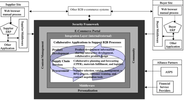
B2B EC systems are a Web-based client/server application designed to facilitate the transfer of purchase orders and other data among different trading partners: suppliers, buyers, alliance partners, and other B2B e-commerce systems (Figure 1). The security framework provides
individual participant a secured and private environment, enabling buyers and sellers manage their own content at their respective extranet. The e-commerce portal builds a personalized content management environment, allowing members, either for free or at a fee, to read and exchange white papers market analysis, production reports, and forecasts, latest industry news, regulatory information and more. Data exchange is via the integration layers. The internal integration integrates multiple applications, legacy systems, databases and data warehouses across the entire enterprise system. The external integration allows the members of different B2B e-commerce systems use different technologies to communicate with one another. The
collaboration applications provide a set of central, online functionality to streamline and
integrate supply chain, enable collaborative product development, and monitor and control the whole procurement process as well as provide market-making function helps to run Web-based B2B auctions and exchanges.
Figure 1. Technology Architecture of B2B EC
Table 1 gives taxonomy of B2B EC systems. The web procurement systems create direct computer links to a company’s dedicated industrial trading partners so order forms and catalogs are readily accessible online. The focus is put on a single, well-established company, such as Procter & Gamble, that develops a web-enabled procurement system to integrate its entire procurement process with selected trading partners. Since the relationship between suppliers and buyers are already built under a long-term contract, the environment uncertainty is relatively low; however the trading partners may often face high lock-in costs. Company’s own e-marketplaces are implemented by an industry leader that does its purchases through its own B2B e-commerce centers. Many of the best-known players in this arena, such as Wal-Mart’s RetailLink, started out by developing their own B2B e-market and aggregating suppliers to compete on price. These e-marketplaces are easier to build and operate because there is a clear leader in the technical and business development. It also has the financial backing of the dominant company, which enables them to move ahead quickly without worrying so much about short-term profits. However, they are less democratic and whether the pricing mechanism is fair to suppliers is often questioned.
Supplier Site Web browser manual process Supplier ERP Other Application Su ppli er Mi ddlew ar e Supplier Site Web browser manual process Supplier ERP Other Application Su ppli er Mi ddlew ar e Buyer Site Web browser manual process Buyer ERP Other Application Bu ye r Midd leware Buyer Site Web browser manual process Buyer ERP Other Application Bu ye r Midd leware
Other B2B e-commerce systems
Security Framework Alliance Partners ASPS Financial Service Providers Alliance Partners ASPS Financial Service Providers E-Commerce Portal Personalization C o nt en t M a n age m ent Com m un it y
Integration Layer (internal/external)
Middleware
Collaborative planning and forecasting (CPFR), materials fulfillment, and logistics
Product
Product
Development
Development
Procurement
Procurement Supplier selection, catalog management,
e-RFQ process, customer training, and contract negotiation tools
Collaborative Applications to Support B2B Processes
Collaborative Applications to Support B2B Processes Product development information sharing, interactive development, collaborative product design
Supply Chain
Supply Chain
Services
Industrial consortium, such as the auto industry’s Covisint, were developed by groups of companies in the same industry. Jointly owned by the largest industry players, they have the advantage of aggregating purchasing power, but they also have their challenges. Trading partners may struggle to collaborate while competing fiercely for customers, because most of them are not willing to reveal sensitive or proprietary information to their competitors. In addition, the
consortium itself is often the target of government anti-trust claims. Table 1. Taxonomy of B2B EC Systems
B2B EC Systems
Features Example Partner’s participation risks
Web Procurement Systems
• Building direct links with dedicated suppliers • Low uncertain about the
revenue
• Low development costs • High connection costs
P&G, Dell • High lock-in costs
• Decreased bargaining power against buyers
• Integration issues with back-end systems
Company’s own
e-marketplaces
• Owned and operated by a single, dominant buyer • Mid uncertain about the
revenue
• High development cost • Low connection cost
Wal-Mart’s RetailLink
• Less democratic, one buyer decides the technical and business development • Intense pressure on price
margins
• Pay a commission for the privilege of selling Industrial
Consortium
• Developed by groups of buyers in the same industry
• High uncertain about the revenue
• Medium development cost
• Low connection cost
Covisint, Transora
• Intense pressure on price margins
• Pay a commission for the privilege of selling
• Reluctant to share planning and inventory information
• Turning over their connection to their customers to the exchange
1.3 Research Questions
As indicated above, the risks involved in the participation make trading partners’ attitude toward B2B EC participation full of uncertainties, especially in the initial stage of system development. It causes two problems for the organization to estimate their investment value. First, the predicted benefits may not occur if the participation is not enough. However, the traditional capital
actually occur, not allowing for problems with conversion effectiveness (Locus 1999). Second, NPV assumes that the interest rate is constant and has no variability. But, if we view the development of ISEC systems as a form of ‘two-stage project’, whether the partners choose to use the system (second stage investment) adds value to the owner company’s infrastructure investment (first stage investment). The variability in the partner side should be different from the developer side. Thus, the adopter is easily biased against funding the B2B EC systems by using NPV analysis. To solve the problem, a more promising evaluation approach with the concern of partner participation uncertainties should be built.
Three research questions are expected to answer in this paper: (1) What are the important determinants of B2B EC participation?
(2) Is there any effective approach to estimate the investment value of B2B EC systems while taking the industrial trading partners’ action and competition pressure into concern?
(3) What is the best investment strategy that the developer can choose to enhance the overall payoff for both participants and itself?
2. LITERATURE REVIEW
2.1 IT Payoff Research
Traditional IT payoff research focuses on well-known financial measures, such as the return on investment (ROI), net present value (NPV), the internal rate of return (IRR), and the payback period. These methods may be suitable to measure the value of simple and intra-organizational IT applications, such as transaction processing and office automation systems within single or several business units (Martinsons, Davison, and Tse 1999). However they are not as well-suited for systems that across business boundaries, where uncertainty and risks is added to the situation as the investment payoffs are no longer depend only on internal contingencies but also on the decisions of trading partners (Chang and Chen 2004, 2005, and Gebauer and Buxmann 2000). Those methods, with the constant interest rate, assume all the predicted benefits will actually occur, not considering the risks or opportunities created by stopping, decreasing, or increasing investment due to the responses of adopters (Locus 1999, Kohli, and Sherer 2002). Its capability to assess IOS value is thereby limited (Benaroch and Kauffman 1999, 2000, Chang 2002, Chang and Hsuan 2005).
Facing the limitations of traditional financial accounting measures, there is another group of researchers uses the process-oriented approach to IT payoff assessment, in order to demonstrating the importance of understanding the process changes that must support payoff (Kohli and Sherer 2002). Balanced scorecard is one representative work (Kaplan and Norton 1992, 1993, 1996), which provides a hierarchical framework to link the strategic activities with company’s financial performance. Furthermore, they extend their valuation analysis from internal business processes to customer satisfaction, the ability to learn and grow, and the shareholder values to offer a complete view of business performance and provide metrics for potential competitive impact other than cost effects. Although this approach attempts to establish the association between
different levels of measures, ex, direct level and indirect level, however it doesn’t investigate the equations that the firms can link the operational improvement to financial performance, and thus limits the practical value. In addition, the intermediate variables such as inventory turnover and cycle time reduction were selected to capture the IT value across the functional areas. It does not consider the impacts across the units and organization boundaries (Barua, Kriebel, and
Mukhopadhyay, 1995).
Since there are drawbacks while solely using firm-level financial analysis or process-level analysis, some researchers suggested the use of Real Option models to deal with the uncertainties of IT investments (Benaroch and Kauffman 1999, 2000). Those approaches explicitly consider the variance of the expected rate of return on the project and thus have the potential to take the uncertainties of IOS investment into account. There have been a lot of attempts made to apply option theory to IT investments. Santos (1991) applied Margrabe exchange option model (1978) to determine the value of ‘second-stage’ IT projects. Two years later, Kambil, Henderson and Mohsenzadeh (1993) introduced the option perspective to establish a linkage between many categories of IT investments and business value. Kumar (1996) made a note to compare the difference between Black-Scholes model (1973) and Margrabe model in the treatment of the cost of the ‘second-stage’ project. Zhu (1999) introduced Geske compound option model (1979) to treat IT investment projects as a sequence of growth options. The most current development is from Benaroch and Kauffman (1999, 2000). They applied Cox and Robinstein binomial option pricing model (1985) and Black-Scholes models to evaluate IT investment, with a real case study on the Yankee-24 electronic banking network.
Although there is a growing research to apply real option approach to IT investment (Martinsons, Davison, and Tse 1999), few research put it into IOS or e-business context (Chang 2001, Chang et al. 2005). Compared with financial and process models such as NPV models and Balanced Scorecard models, we think real-option approach provides a better approach to identify the uncertainties involved in IOS investment. However substantial modifications should be made to reflect the IOS environment. The changes stem from our view that: (1) the perspective of participants (i.e. supply chain partners) has to be taken into consideration. (2) IOS projects are commonly carried out for the benefits of both focal companies and the trading partners as a whole (rather than individual company within a large market). We will introduce the new modeling efforts in the next section, but before that alternative real-option models are summarized below.
2.2 Review of Real-Option Models
The binomial and Black-Scholes are two basic, most commonly used models in pricing financial options. In the following, a brief review on both models will be introduced. Furthermore, since our focus is on IT payoff evaluation, the applicability of each model to IT investment will be highlighted.
2.2.1 Binomial Model
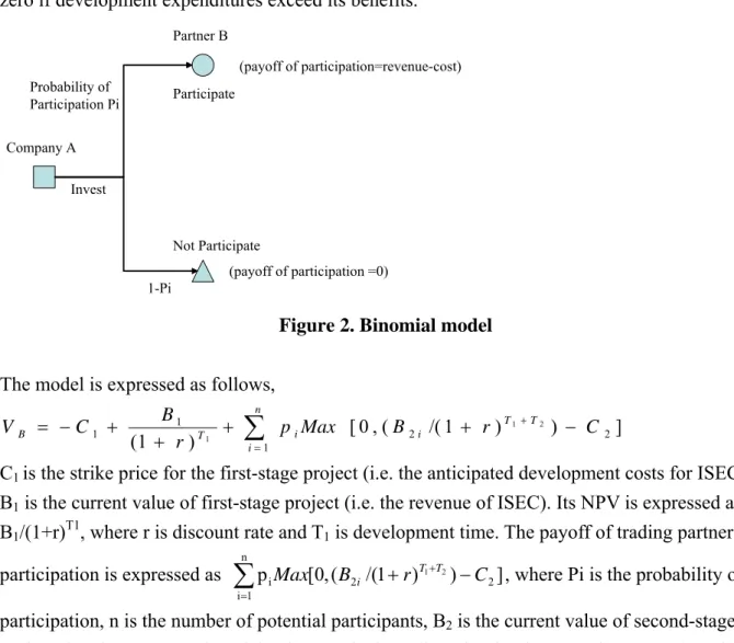
The option thinking can be used to construct decision trees using the NPV method (Figure 2). After company A invests the ISEC, trading partners have the option to participate or not. Partners
will not participate if revenues do not exceed development costs, therefore the true expected value of ISEC when participation options are considered will be no less than the value if
participation options are not considered. The payoff on partner’s participation is the maximum of zero if development expenditures exceed its benefits.
Company A Invest Not Participate Partner B Probability of Participation Pi Participate
1-Pi (payoff of participation =0)
(payoff of participation=revenue-cost)
Figure 2. Binomial model
The model is expressed as follows,
] ) ) 1 /( ( , 0 [ ) 1 ( 1 2 2 1 1 1 p Max B r 1 2 C r B C V i T T n i i T B + + − + + − = + =
∑
C1 is the strike price for the first-stage project (i.e. the anticipated development costs for ISEC).
B1 is the current value of first-stage project (i.e. the revenue of ISEC). Its NPV is expressed as
B1/(1+r)T1, where r is discount rate and T1 is development time. The payoff of trading partners’
participation is expressed as n p [0,( 2 /(1 ) ) 2] 1 i iMax B r 1 2 C T T i + − + =
∑
, where Pi is the probability ofparticipation, n is the number of potential participants, B2 is the current value of second-stage
project (i.e. the revenue of participation), C2 is the strike price for the second-stage project (i.e.
the anticipated development costs incurred in the partner side) and T1 is the participation cost.
To access the applicability to IT investment, this approach has the difficulties in determining an appropriate discount rate for new IT projects. Ideally, the discount rate used should be based upon the risk of the asset created by the investment. This rate may be set by finding a
market-traded investment of equivalent risk and using its rate of return. Determining a rate in this manner is very difficult, because the risk of the option is non-stationary, i.e., it changes with time to expiration. Even if the discount rate is assumed to be stationary, determining an appropriate discount rate is difficult. Ideally, one would have to find a firm whose only asset is the same as the asset this project will produce. This is almost always impossible. Hence, discount rates are almost never set in this manner. Instead, firm often uses their cost of capital or some other rate for all projects. Since project risk varies across investments, setting rates in this manner favors high-risk projects. To compensate, discount rates set by managers are extremely high, far in excess of what is reasonable. High rates favor projects with large short-term cash inflows and penalize those projects where cash inflows are spread out over a longer period. This is most often the case with new IT investments where large payoffs may not be seen for several years (Santos
1991).
2.2.2 Black-Scholes Model
The options approach described here can help overcome some problems addressed in binomial models. If we assume the participation is a deferral option, the value of participation is expressed as follows, ) 5 . 0 ) / ln( ( ) 5 . 0 ) / ln( ( 2 2 2 2 2 2 1 2 2 2 2 2 2 2 2 1 2 2 2 2 t t t rt C B N e C t t rt C B N B VB rt σ σ σ σ σ + − + − = −
The function, N, is the cumulative normal distribution. σ is the variance of the expected payoff
from participation. Compared with the binomial model, an apparent strength of Black-Scholes is its computational simplicity; it has a closed-form solution. This, in turn, makes it easy to conduct sensitivity analysis using partial derivatives.
In addition, the Black-Scholes has a better way to deal with company’s capability to defer the investment. The possible investment value based on the usual binomial decision rule: “Don’t invest if NPV is negative”, implying a kinked payoff line that is coincides with the value line of a call option, but only if the option were one that matures immediately (i.e., the case if the
company had a “now-or-never” type of investment). Thus, binomial model can be said to
recognize the value of embedded deferral options, but only when the options mature immediately. By contrast, the Black-Scholes pricing analysis takes into account the fact that changes in
revenue expectations will occur as time passes. No parameter adjustments (e.g., discount rate or the expected value of revenues) are needed. Instead, these models incorporate this kind of
information by explicitly considering the asymmetric distribution of expected revenues, and their perceived variability. This is accomplished with a model parameter that is referred to as
“volatility” in the finance literature; it reflects the variance of the expected rate of return on the project.
However, from a practical standpoint the data required for Black-Scholes are just as difficult to develop as for binomial analysis. The analysts still have to estimate the variance in the
expected return on the IT investment. But the model does take the variability of expected returns, or risk, from the project into account, while binomial model uses one risk-adjusted discount rate that applies equally well to all different scenarios.
Some experts in finance argue that Black-Scholes models should not be used for nontradable assets. Do IT investments “trade”? What is the value of a partially finished IT project, or what is its salvage value? Is there a market for such projects? In financial options valuation one can ignore the option’s risk because the stocks underlying options can trade as well. As a result, one can price the option from the price of the underlying stocks, whose price itself reflects the risk and the investor’s risk aversion. The investor can always hold some quantity of the underlying stocks to hedge this risk. Facing these issues, Locus (1999) defended the option pricing approach by stating that “…In applying models it is not unusual to violate one or more of their assumptions. The issue is whether or not the violation is material; does it lead to incorrect conclusions and results? … Unlike the options pricing specialist, the manager confronting an IT investment is not
pricing a stock option for purchase or sale. Instead, this manager seeks guidance on making an investment.” Therefore, we think the option pricing models will treat the B2B EC investment better with their ability to model asymmetric returns and to recognize the value of deferral investment (Benaroch, Kauffman 1999). Our modeling process is detailed in the following section.
3. MODELING THE INDUSTRIAL TRADING PARTNER PARTICIPATION AS CORPORATE REAL OPTIONS
By analogy, an investment in a B2B EC system can be considered as two nested options. Similar as the first option will give its holder the right to buy the second option by paying the fist striking price, investment in a B2B EC infrastructure will give the initiator the ability to attract industrial trading partners to join by paying its development costs. Just as the second option gives the holder the right to acquire the stock by paying the second strike price, trading partners’
participation will give the initiator expected revenues by paying the connection costs. Further, just as the investor can choose not to exercise the option on the first exercise date (if the option on that date is lower than the first strike price) or on the second exercise date (if the option on that date is lower than the second strike price), firms can decide not to initiate B2B EC development and their trading partners can choose not to participate. Thus, the trading partners’ participation is equivalent to the stock on which the compound option is written, while the investment in the B2B EC is similar as purchasing the right to write an option contract.
The binomial and Black-Scholes models described in the last section only consider a ‘plain’ option, where no nested options are embedded. As indicated above, B2B EC investment involved at least two options (i.e. initiator’s option and partners’ option), so we need advanced models which relax some of the limitations of the basic models. In this proposal, we introduce Geske compound option model (Geske 1979), which is derived from Black-Scholes model but is able to value nested sequence of options (i.e. compound options). The model is built around the concept that the exercise of one option leads to the exercise a specific option in the next stage, quite similar as the sequential nature existed in the B2B EC investment.
Zhu (1999) has mentioned the applicability of Geske model to the IT investment, but the paper did not apply it in the inter-organizational environment. Latter on, Chang (2001) applied the Geske model in a game-based valuation framework to consider the suppliers’ payoffs of buyer-based e-marketplaces. With the reference of both research works, we add the participation variability into the model and eliminate the constant interest rate. We also consider the time variability during the development and participation stage. In addition, we attempt to propose a measure system to combine the user-oriented valuation studies (, which the focus is on
“user-oriented benefits and costs”) with the option valuation models. The model is described as follows.
) ( ) ; , ( ) ; , ( 1 2 2 2 1 1 2 2 1 1 1 1 2 d d C e 2N d T d T Ce 1N d T BN VC = ρ − −rT −σ −σ ρ − −rT −σ where
1 1 2 * 1 ) 2 ( ) / ln( T T r B B d σ σ + + = , 2 2 2 2 2 ) 2 ( ) / ln( T T r C B d σ σ + + = , ρ = T1 T2 and B* =[C2e−r(T2−T1)N1(a−σ T2 −T1)+C1] N1(a) where 1 2 1 2 2 2) ( 2)( ) ln( T T T T r C B a − − + + = σ σ
The function, N1, is the cumulative normal distribution, and N2 is the cumulative bivariate normal
distribution function. The variable B2* is the threshold value of B above which the compound
option should be exercised1. Other notation is explained below:
VC: the payoff of the compound option (i.e. the payoff of B2B EC investment)
B: the current revenue of the entire project (i.e. B2B EC’ revenue after partners’ participation) C1: the strike price for the first-stage project (i.e. the anticipated development costs for initiating
B2B EC systems)
C2: the strike price for the second-stage project (i.e. the anticipated connection costs incurred at
the partner side)
σ2: the variance of the expected revenue from the entire project, computed as σ2
B+ σ2C-2 σB σC
ρBC; σ2B is variance of the rate of change of revenue, σ2C2 is variance of the rate of change of
cost, and ρB2C2 is correlation between development costs and revenues2.
T1: The first exercise date (i.e. the time before which the option to develop the B2B EC must be
exercised)
T2: The second exercise date (i.e. the time before which the option for the partners to participate
in the B2B EC systems must be exercised). r: the risk-free interest rate
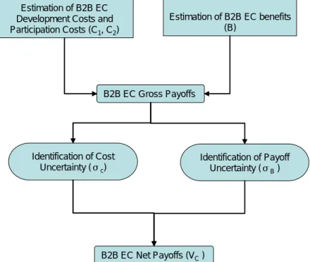
Based on the model, the process to calculate the payoffs of B2B EC investment involves three steps: (1) estimation of B2B EC development costs and benefits, (2) define the uncertainties and risks along the development, and (3) identify the competitive pressure. In what follows, I explain these steps and illustrate them in the following figure.
1 B* is the value of the underlying asset (i.e. the value of B2B EC) at time T
1, for which the compound option value (V) at time T1 equals X1. If the actual B is above B* at time T1, the first option will be exercised; if it is not above B*, the option expires worthless (Hull, 2000).
2 The value of ρ
BC depends on how much revenue draws from costs. To simplify the computation, we assume it is zero.
Estimation of B2B EC Development Costs and Participation Costs (C1, C2) Estimation of B2B EC benefits (B) B2B EC Gross Payoffs Identification of Cost Uncertainty (σc) Identification of Payoff Uncertainty (σB) B2B EC Net Payoffs (VC)
Figure 3. Proposed Process of Calculating B2B EC Payoffs.
Step 1: Estimation of B2B EC Development Costs and Benefits
The first step entails estimating the development costs and payoffs. Gebauer and Buxmann (2000) define two cost types of B2B EC. One time setup costs are the costs related with the installation of the technical and organizational infrastructure. For the companies that initiate the B2B EC, the one time setup costs includes all hardware and software expenses necessary to the setup of the system and the manpower and training costs for preparation of the organization for using the system, independent of the links with specific partners. For the partners that connected to the system, the one time setup costs are the expenses related to the establishment of business
relationship, configuration, and customization. Current costs occur after one-time setup and on an ongoing basis. They are the costs related with the use and maintenance of the system, including the costs for enhancing software solution and leasing and network access fees. The current costs occur at the initiator’s side as well as at the participants’ side.
The body of research that evaluates the payoffs of B2B EC is large and diverse. It can be summarized into three groups. The first group examines the value of B2B EC from the point of
technology standardization. A new dimension – network effect - is added into the situation to
show the relationship between the value of the standardization and the installed base of such technology standards. For example, Kauffman, McAndrews, and Wang (2000) used electronic banking as a context for examining shared network effects. They argued that as more suppliers joined the network, existing users would value the systems more highly because of increased convenience and enhanced access. The second group comprises the work attempting to gauge the operational value of B2B EC and puts emphasis on the internal business processes, e.g., the impact on inventory turnover and quality, shipping discrepancies, and order processing (Zhu and Karemer 2002, Zhu 2004, Ravichandran and Lertwongsatien 2005). The third group puts the interests on external factors that may mitigate the business outcome, specifically with regard to
exploiting IOS capability to leverage relationships with business partners. Some researchers identify the uncertainty and risks within the interorganizational relationships and related them to the success of the IOS (Gebauer and Buxmann, 2000). Others define strategies of fitness between environment need and B2B EC (Premkumar et al. 2005) and examined strategic implications of B2B EC, including how B2B EC enables a firm to maintain its overall cost leadership, improves the business or manufacturing processes between firms in the supply chain, adds value to customers, and enhances the dependence of customers and suppliers on the firm (Wheeler 2002, Schultaze and Orlikowski 2004, Zhu et al. 2005).
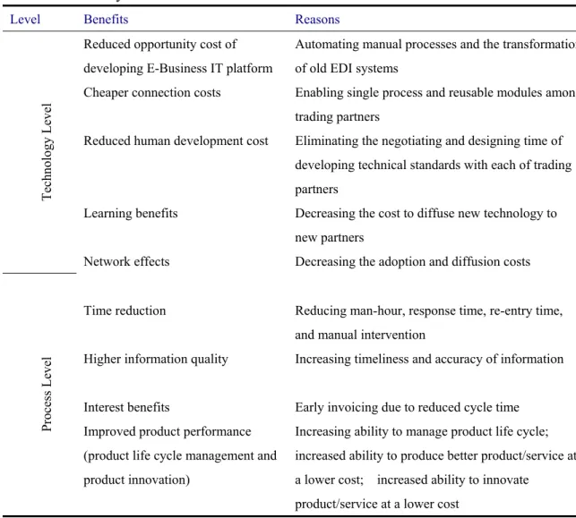
Table 2 offers a summary of B2B EC benefits identified by three research streams. As suggested earlier these benefits can be placed into three categories.
z Technology value refers to the savings due to the reduction of IT personnel costs for using the system as the system becomes more flexible and interoperable.
z Process value is the reduction of process time and cost due to the IT-enabled operational improvement.
z Relationship value is the result of better customer service and improved trading partner relationship enabled by B2B EC.
Table2. Summary of B2B EC Benefits
Level Benefits Reasons
Reduced opportunity cost of developing E-Business IT platform
Automating manual processes and the transformation of old EDI systems
Cheaper connection costs Enabling single process and reusable modules among
trading partners
Reduced human development cost Eliminating the negotiating and designing time of
developing technical standards with each of trading partners Tech nol og y Le vel Learning benefits Network effects
Decreasing the cost to diffuse new technology to new partners
Decreasing the adoption and diffusion costs
Time reduction Reducing man-hour, response time, re-entry time,
and manual intervention Higher information quality
Interest benefits
Increasing timeliness and accuracy of information Early invoicing due to reduced cycle time
Process Le
vel
Improved product performance (product life cycle management and product innovation)
Increasing ability to manage product life cycle; increased ability to produce better product/service at a lower cost; increased ability to innovate
Reduced Inventory holding and obsolescence costs
Increased capacity utilization
Reducing demand variability and improving forecast accuracy
Improving the visibility and better planning the production
Better Sales from improving customer satisfaction
Fast time to markets; better fulfillment rate; better customer services
Improved customer retention rate Easier for the customers to collaborate with its suppliers
Reduced coordination costs with trading partners
Improving trading partner’s asset utilization and reducing their overhead by fewer line stops Increased quality of supply
offerings
Reducing lead-time for delivery; improving on-time delivery; reducing the defect rate
In
ter-Fi
rm
Lev
el
Better supply price Lower shipping costs; lower costs to respond to RFQ
Step 2: define the uncertainties that add to the variability of payoffs
As most B2B EC aims at facilitating the collaboration in supply chain and demand chain relationships, the benefits must depend on the way in which its trading partners implement and use the technology, thereby uncertainty/risks becoming a critical contingency. Kumar and van Dissel (1996) identified three arguments to explain the potential for cooperation and conflict between the participants in the collaborative alliance: economic relationship, technical feasibility, and socio-political considerations. These three perspectives help us identify where risks occur. We generalize and expand them to the broader context of explaining the possible risks in implementing B2B EC.
Transaction-specific Risks are the costs associated with transacting in the company’s value
chains via B2B EC. Based on Kumar and van Dissel (1996), the risk of losing resource control may occur as company’s key information resources such as strategic data and knowledge
know-how are transferred with part of the transactions. In other words, companies may hesitate to share information resources that have greater value of competitors such as factory capacity, product specification, and engineering data unless they are confident that the system is secured. The fear of losing their competitive advantage can add the complexity to e-Business IT
implementation. Moreover, the supply chain collaboration enabled by B2B EC changes the way that organizations used to manage the interactions, which we term collaboration structure. Such changes can improve overall supply chain / demand chain efficiency, but can also affect the bargaining power of the parties. In some cases, trading partners may find themselves actually worse off under improved coordination, due to a loss of bargaining power, and thus leading them to resist the change (Clemons and Row, 1993). Since these transaction-specific risks increase the participation uncertainties of B2B EC, we can expect they affect the ability of the investing firm to successfully realize the payoffs of B2B EC investment. Further, the investment of a
profitability of B2B EC. Such asset specialty makes companies neither easy nor costless to shift across network sub groups and therefore company’s return may vary with the network it is locked in (Clemons and Row 1992, Kumar and van Dissel 1996).
Relationship-specific Risks are related with the costs of managing inter-organizational
relationships. B2B EC, like other types of IOS innovations, can’t be adopted and used unilaterally. Firms that are motivated to begin using e-Business IT must either find similarly motivated
partners, or persuade or coerce their existing market partners into adopting the technology. Additional time is needed to gain agreements with trading partners about the structure and meaning of data. Moreover, once the technology has been adopted, firms must continue to invest in the technology and implement additional transaction sets to gain coordination benefits. All of those require more coordination from trading partners, thereby incurring more coordination costs that affect the payoffs expected from the investment opportunity. Besides coordination costs, interest conflict with participants in the collaboration, which we call socio-political risks, might also discourage the willingness to make investment, and thus affect the ability of the investing firm to obtain the payoffs (Hart and Saunder 1998).
Competition Risks refers to the situation that a competitor may make a preemptive move, or
simply copy the investment and improve on it (Benaroch 2002). The initiators of B2B EC can always adopt a “wait-and-see” approach to gain the option value of waiting. However, its wait may give other competitors the chance to invite the suppliers. The same strategic concern can be applied to the supplier too. The supplier can always wait till the condition becomes more certain and positive, but during its wait, other suppliers who participate earlier then get more access to the buyer. Therefore, these risks give rise to the possibility that the investing firm might lose the profitability expected from the investment opportunity.
Step 3: identify the risks that add the variability of costs
These risk factors refer to those that affect the speed and cost to implement B2B EC. We have identified two type of costs related with the development, maintenance, and use of the B2B EC. Clearly, to the extent that the availability of such B2B EC infrastructure is uncertain now or in the future, the variance that affects the expected costs of B2B EC will be greater. Scholars have defined three categories of infrastructure supporting the system development: physical
infrastructure, social infrastructures, and human capital infrastructure (Becker 1964, Itami 1987, Rosenkopf and Tushman 1994). Physical infrastructure contains the necessary
network/telecomm connection, platform compatibility, data/application modularity, and so on. Social infrastructure includes commonly accepted business practices or standards supporting B2B EC. Human capital infrastructure consists of the managerial and technical skills available for developing B2B EC. We can expect the lower the availability of these infrastructure, the higher the cost variability will be.
On the other hand, the complexity of technical infrastructure may lead to the slow
development and adoption, thereby adding the cost variability. We can expect the complexity of B2B EC technology can function as an inhibitor to adoption and it can also inhibit further diffusion, since the organization may not be able to easily integrate it with the rest of the
organization (Premkumar et al. 1994), and the complexity of the technology gives rise to the possibility that the system can not work or can’t be completed on schedule or within budget, with adequate performance. It is wide common in B2B EC implementation that one of the partners may perceive supply chain collaboration to be very complex and may lack the technical
capability to install the system in its firm. Even if the firm adopts the technology due to market pressure and help from trading partners, the usage may be limited to simple electronic
transmission and may not be integrated with other IS applications, thereby not obtaining significant payoffs expected from investing B2B EC.
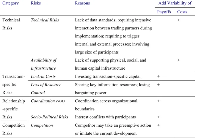
Table 3 summarizes our proposed risk portfolio that affects the payoffs and costs of B2B EC investment.
. Table 3. Risk Portfolio in Supply Chain Collaboration Enabled by E-Business IT Add Variability of
Category Risks Reasons
Payoffs Costs Technical Risks Lack of data standards; requiring intensive
interaction between trading partners during implementation; requiring to trigger internal and external processes; involving large size of participants
+ Technical
Risks
Availability of Infrastructure
Lack of supporting physical, social, and human capital infrastructure
+
Lock-in Costs Investing transaction-specific capital +
Transaction-specific Risks
Loss of Resource Control
Sharing key information resources; losing bargaining power
+
Coordination costs Coordination across organizational
boundaries
+ Relationship
-specific
Risks Socio-Political Risks Interest conflicts with participants +
Competition Risks
Competition Competitor may take an preemptive action
or imitate the current development
+
4. MODEL APPLICATION: AN INVESTMENT DECISION OF DEPLOYING ROSETTANET-BASED B2B EC
The case company is a world leading manufacturer of computer networking and communications products, conducts more than 30,000 transactions per month with more than 90 customers and suppliers who are based in 17 countries and mostly in Asia. The lack of visibility across its supply chain is its main cause of inefficiencies which accelerate supply and demand mismatches. These mismatches are leading to poor capital efficiency, missed commitments, inventory excesses or shortages and increased costs. To address the unique order management needs of the semiconductor manufacturing supply chain, the case company, in 2001, considered to streamline
its procurement process with its component and assembly subcontractors by implementing RosettaNet-enabled e-procurement solutions.
Both the case company and its subcontractors knew that automating procurement would provide broad range of benefits for both partners. First, the RosettaNet-enabled e-business IT infrastructure supports interoperability among different systems within the enterprise. Users have the flexibility of accepting multiple messaging formats and data transport languages from both new and existing technologies. Second, collaborative process technology enables general industry and company-specific information exchange to all authorized members. Companies and their suppliers are able to share real-time information and exchange ideas for decision management and knowledge sharing, improving the timeliness of choices made, as well as internal and external communication and coordination, and facilitation of organizational learning. Third is the simplified procurement process achieved by simultaneously connecting all parties to facilitate the real-time collaboration. Faster constraint visibility and resolution reduce overall inventory and cycle time.
While RosettaNet implementation is expected to provide better value than traditional IOS, it also incurs some costs. The case company had to consider three uncertainties related with supplier participation: uncertainty about the participation, uncertainty about the connection costs, and uncertainty about the time to participate.
Participation uncertainty: The participation uncertainty directly affects whether the expected revenue will be achieved. The environment surrounding the supplier and the organization relationship may force or encourage the participation. We discuss three sources of such participation uncertainty. First is the switch cost. As the supplier has a lot of investments highly specific to the relationship, it is costly for the supplier to switch to another buyer. Second is the length of the contract. If the supplier has a long-term relationship with the company, it means there exist a direct or indirect promise of guaranteed volumes and repeat business, which reduces the supplier risk to participate. The last is the ownership participation. The higher the ratio is, the deeper engagement is between the supplier and the buyer, and the less risk for suppliers to participate.
Cost uncertainty: The flexibility of the supplier IT resource, such as network/telecomm connectivity, platform compatibility, and data/application modularity, and the level of intra-process or inner-process information sharing affect the cost and time to incorporate the e-commerce systems into the organization IT infrastructure, and thus affect the value realization of participation. We discuss two uncertainties related with supplier IT infrastructure: (1) the flexibility of IT and (2) the level of information sharing.
Time uncertainty: After supplier decides to participate, the next question for them is when is the best time to join. The time may vary depending upon the trusting climates between the supplier and the buyer. A good trusting climate can reduce the supplier’s doubt about the buyer proposed benefits and therefore shorten the time to participate. The trusting climate can be measured by the number of training programs offered to the suppliers for using the B2B e-commerce systems, the availability of incentives offered to the suppliers to adopt the systems, and the average responding time to supplier’s technical requests.
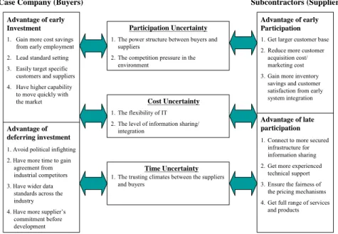
Those uncertainties directly affect how the buyers design their investment strategies. There are several key decisions involved in the development process of buyer-based B2B e-commerce systems. The case company has to decide when to develop the system and estimate the expected return after the supplier participates. There are also two decisions for the supplier: the time to participate the systems and the connection costs to the e-commerce systems. Both supplier and buyer will choose the strategy, which can bring her the best payoffs. The advantage for each timing strategy is summarized in Figure 3.
Case Company (Buyers) Subcontractors (Suppliers)
Advantage of early Investment Advantage of early Participation Advantage of deferring investment Advantage of late participation Participation Uncertainty Cost Uncertainty Time Uncertainty
1. Avoid political infighting 2. Have more time to gain
agreement from industrial competitors 3. Have wider data
standards across the industry 4. Have more supplier’s
commitment before development 1. Gain more cost savings
from early employment 2. Lead standard setting 3. Easily target specific customers and suppliers 4. Have higher capability to move quickly with the market
1. Get larger customer base 2. Reduce more customer
acquisition cost/ marketing cost 3. Gain more inventory
savings and customer satisfaction from early system integration
1. Connect to more secured infrastructure for information sharing 2. Get more experienced
technical support 3. Ensure the fairness of
the pricing mechanisms 4. Get full range of services
and products 1. The power structure between buyers and
suppliers
2. The competition pressure in the environment
1. The flexibility of IT 2. The level of information sharing/
integration
1. The trusting climates between the suppliers and buyers
Figure 3. The summary of advantages for alternative investment strategies
4.1 Choosing a Pricing Model for Alternative Investment Strategies and Eliciting Model Parameters
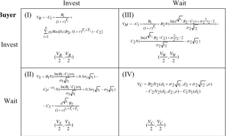
Based on the previous discussion, we define four investment-timing scenarios and show the payoff in Figure 2.
(I) The case company decides to invest the infrastructure immediately and the supplier then decides to participate immediately after the infrastructure is built:
Both players don’t consider deferred entry: there is no deferral option in both sides. That means both options are exercised immediately. Past literature (Cox and Rubinstein 1985, Santos 1991, Benaroch and Kauffman 1999) formulated this scenario as a Cox and Rubinstein binomial option pricing problem, assuming both options are matured immediately and the payoff on a second-stage project is the maximum of zero if development expenditures exceed its benefits (i.e. the supplier will not participate if revenues do not exceed connection costs). VB represents the investment value in this
scenario (Figure 4 (I)). B1 is the expected revenue from the infrastructure development,
independent from the revenue of supplier participation; pi is the probability of supplier
participation; B2i is the value that will actually be realized for each possible outcome of
and the supplier share the option value equally, resulting in a (VB/2, VB /2) payoff for each
firm.
(II) The case compnay decides to defer its investment while considering the uncertainties of supplier participation, but once the investment is made, the supplier participates immediately:
Only the buyer considers deferred entry: the investment possesses only one deferral option at buyer side. Because the development cost is fixed at the time the buyer decides to invest in the B2B e-commerce system, we don’t need to consider the variability of the development costs happened in the company side. It makes more sense to employ Black-Scholes model for its assumed deterministic exercise price and plain option (no nested options involved). VS represents the investment value in this scenario (Figure 4 (II)). σ2 is the variance in its
expected return of the infrastructure investment and e-rt1 is the present value factor for risk-neutral investors. The payoff for each firm is (VS/2, VS /2).
(III) The case company invests the infrastructure immediately, but the supplier defers its participation under uncertainty
In this scenario, the supplier participation is viewed as an option, while the exercise of this option leads to the acquisition of a technology. Different from scenario II, the supplier connection cost is uncertain at the time the B2B e-commerce system infrastructure starts to build. Thus, we can’t take the development cost of the supplier participation as a
deterministic value. It is more suitable to employ Margrabe model, which determines the value of an option to exchange one risky asset for another using stochastic development costs. VM represents the investment value in this scenario (Figure 4 (III)). The payoff for
each firm is (VM/2, VM /2), where is the Margrabe option value plus the expected cash flow
from the B2B e-commerce system infrastructure investment.
(IV) The case company decides to defer its investment, same as the supplier
When both company and supplier decide to wait, it can be seen as a compound option, which has been discussed in section three. Both firms are able to employ deferral option, where the connection costs of supplier participation is uncertain. VC represents the
Figure 4.Payoffs for company and supplier in four investment-timing scenarios
Next, we need to estimate the uncertainties during the implementation. Based on the description above, three uncertainties need to be solved: participation uncertainty, cost uncertainty, and time uncertainty. The estimation of these parameters is described as follows,
A. Participation and Cost Uncertainties
If we assume the variation in B2 and C2 is normally distributed, the σ2B2 and σ2C2 can be
estimated by the following function: σ2
B2 = nB*pB (1-pB)
σ2
C2 = nC*pC (1-pC)
, where nB is the percentage of the fluctuation within the expectation, pB is the percentage of
change above or below the expected value (i.e. B2), and pC is the percentage of change above or
below the development costs (i.e. C2) 3. We can express nB as an implicit function nB = nB (a1, a2,
a3, a4,…, am), where ai (i=1 to m) is the environmental factor affecting the fluctuation of
prediction, the same as nC = nC (b1, b2, b3, b4,…, bk), where bi (i=1 to k) is the environmental
factor affecting the fluctuation of supplier connection costs.
Based on the discussion in section three, nB = nB (switch cost, ownership ratio, contract
length) and nC = nC (IT flexibility, level of integration). If we assume each factor of our interest
has equal contribution and are the only sources to the variability, we can calculate the variability using Cobb-Douglas function4:
3 p
B and pC can be obtained from the subjective estimate of the system development staff.
4 The reason we use Cobb-Douglas production function is because it lies between the extremes of the linear production function and the Leontief production function, assuming some degree of substitutability among inputs. The assumption corresponds to the characteristics of our proposed influential factors here, some degree of correlation among the factors.
Invest Wait Invest Wait Supplier Buyer ] 2 ) ) 1 /( 2 ( , 0 [ 1 ) 1 ( 1 1 2 1 1 C T T r i B Max n i i p T r B C B V − + + = + + + − = ∑ ) 2 , 2 (VB VB 2 1 1 1 1 ) 1 ( 2 2 ) 1 1 1 1 5 . 0 1 1 1 ) 1 / 1 ln( ( 1 ) 1 1 5 . 0 1 1 1 ) 1 / 1 ln( ( 1 T T t r B t d C t t t rt C B N rt e C t t rt C B N B S V + + + + − − + − − + = σ σ σ σ σ ) 2 , 2 (VS VS ) 2 2 2 2 2 / 2 2 2 ) 2 / 2 ln( ( 2 ) 2 2 2 / 2 2 2 ) 2 / 2 ln( ( 2 ) 1 ( 1 1 2 2 1 t t t C B t d N C t t C B t d N B T r B C M V σ σ σ σ σ − + − + + + + − = ) 2 , 2 (VW VW ) 2 , 2 (VC VC (I) (II) (III) (IV) ) 1 ( 1 1 ) ; 2 , 1 ( 2 2 ) ; 2 2 2 , 1 2 1 ( 2 2 d N C d d N C t d t d N B C V − − + + = ρ ρ σ σ
2 1 2 1 3 1 3 1 3 1 I F n C O S n C B = = , where 2 Ext Int I 3 Mod Com Con F + = + + =
S is the switch cost, O is ownership ratio, and C is contract length.5 The IT flexibility is
computed by three resources:
(1) Con is the extent of connectivity, measured by the percentage of end users inside the supplier company are planned to connect to the e-marketplace.
(2) Com is the platform compatibility, measured by the percentage of hardware inside the supplier company can support the e-marketplace.
(3) Mod is the modularity of data, measured by the percentage of applications software inside the supplier company can be transported and reused across the e-marketplace.
The level of IT integration is computed by two resources:
(1) Int is the extent of the internal integration, measured by the extent of integration of the e-marketplace with the back-end supplier system.
(2) Ext is the extent of the external integration, measured by the percentage of transactions implemented via the e-marketplace.
B. The variability of time can be measured using the similar approach.
3 1 3 1 3 1 2 2 t =(1−Tra) (1−Inc) (1−Req) σ
We assume good trusting climates between organization and the supplier contribute to the reduction of time variability. Tra represents the availability of the training programs, Inc is the availability of the incentives, and Req is the average responding time to supplier’s technical requests.
5. ANALYSIS RESULTS
Through in-depth interview and company’s financial reports, we require all the parameters we need for each investment timing model. The payoffs for the case company and its subcontractor in four investment-timing scenarios are shown in Figure 4. When manufacturer adopts a deferral option and supplier chooses to participate immediately, both parties can have highest payoffs.
5 The values of those three factors are normalized, which means each value represents a relative importance of buyer-based B2B e-commerce to all the other IT projects for the supplier.
Figure 4. The payoffs calculated for the manufacturer and the supplier in four investment-timing scenarios using data from case company
The logic behind the results is as follows. The development of B2B EC in the case company involved considerable uncertainty. First is about the participation uncertainties. The
components are not easily interchangeable, which makes the subcontractors very picky and specific. Second comes from cost uncertainties. The high level of supplier fragmentation makes document standardization and process synchronization, such as for ordering and invoicing, across tens or even hundreds of different information systems a daunting task. For example, the case company needs to buy over 400 production components from numerous distributors located across the globe. A third source of uncertainty is time uncertainty. Suppliers may fear that online marketplaces will break up long-standing relationships between them and their customers, which can seriously delay the time they decide to
participate. Those uncertainties may make suppliers to adopt a deferral option. As a result, to make both parties better off, the analysis tells us the manufacturers should have more time to gain the consensus from the suppliers and have more supplier commitment before
development. Manufacturer’s deferral option can digest most supplier uncertainty and encourage their participation.
6. CONCLUSION AND FUTURE RESEARCH
This paper examines the impact of supplier participation uncertainty on evaluating the investment value of B2B e-commerce systems through a game-based option valuation model. The
Invest Wait Invest Wait Supplier Manufacturer (I) (II) (III) (IV) (0.5, 0.5) (1.37, 1.37)** (0.03, 0.03) (1.28, 1.28) Long wait Short wait (-0.11,-0.11) (0.27,0.27) Long wait Short wait Assumption:
1. The infrastructure development costs (C1): capital investment + software investment+employee salary (Assume each manufacturer has equal investment) – (250M+180M)/56+250*30,000)=15.5M
2. B1 -- transaction revenues: 25%*600000M*0.05*0.047=353M, 353M/56=6.3M 3. R: 7% risk-free interest rate
4. Connection cost: $400*5*12*100+100*30,000=4.4M (Assume 100 employees worked on this project. The monthly software subscription fee is $400 for each application. )
5.The expected revenue: 6890M/750=9.2M (Suppose 750 participants) 6. T1=2years
7. T2=0.5 year 8. t1= 1year
9. t2= 2year± z(0.975)* σ t2=0.5±1.96* σ t2
10. σ: Pb--75% (conservative prediction), Pc=0.5, s:0.1, c:0.1, o:0.1, con:0.1, com:0.1, mod: 0.1, int:0.1, ext:0.1, tra: 0.1, inc: 0.1, req: 0.1
11. d=0.25
Payoffs for Manufacturer
-0.2 0 0.2 0.4 0.6 0.8 1 1.2 1.4 1.6 1 2 3
The time supplier joins e-marketplace
M a n u fa c tu re r P a y o ff (M illio n ) invest wait
contribution of this research is multi-folded: First, the research applies the compound option model to improve the pitfalls of traditional NPV approach and plain option models (ex: Black and Schole’s model), so uncertainties can be considered both in the buyer side and the supplier side, which is more related with B2B e-commerce system investment. Besides that, we also enhance the original compound option model by adding the time variability and development cost variability, so the uncertainties related with supplier lock-in costs and time to the market can be considered while estimating the investment value. In addition, we develop a measurement system to estimate the variability, linking the user-oriented benefit/cost studies with the option models. For example, to effectively estimate the variability of expected revenues in the option model, we suggest the use of three measures: switch costs, ownership ratio, and contract length. Although the validity of those measures has to be further justified, the approach provides a practical way to estimate multiple variances in the option model. At last, we add the dimension of competitive advantage by using the game theories, which gives us a way to evaluate the counteraction between the suppliers and buyers.
However, the model has its limitations. We have to assume the buyer and the supplier have the same reasoning of thinking. In the traditional compound option model, the first option and the second option is bought by the same company, but now the first option is from the buyer and the second option is from the supplier. Since it is common in the economic theory to assume everyone will choose the behavior that is best to herself. This assumption should not affect our evaluation results too much. Secondly, we only consider the competition and uncertainty in the supplier side. However, for some e-marketplaces, the founders are the competitors in the same industries. The uncertainties and the competition among those industrial competitors should also affect the investment decisions. As a result, the model presented here can be extended to a
two-stage game in the future where the competition between the buyers can be viewed as the first stage game and the equilibrium derived affects the second stage game that is the competition between the suppliers.
REFERENCES
Barua, A., Kriebel, C., and Mukhopadhyay, T., “Information Technology and Business Value: an Analytical and Empirical Investigation,” Information Systems Research, 6,1, March 1995, pp. 3-23
Benaroch, M., and Kauffman, R., “A Case for Using Real Options Pricing Analysis to Evaluate Information Technology Project Investments,” Information Systems Research, 10, 1, March 1999, pp. 70-85
Benaroch, M., and Kauffman, R., “Justifying Electronic Banking Network Expansion Using Real Options Analysis,” MIS Quarterly, 24, 2, June 2000, pp. 197-225.
Black F. and Scholes M., “The pricing of options and corporate liabilities,” Journal of Political
Economy, (81:3), May-June 1973, pp. 637-654.
Chang, H. and Hsuan, C., "Developing A Framework for Measuring the Supply Chain
Capability," IACIS Pacific 2005 Conference Proceedings, International Association for
Computer Information Systems, Taipei, May 2005 [supported by NSC
93-2416-H-004-021]
Chang, H., Chiu, I., Hsuan, C. and Weng, H., "Using Option Valuation Approach to Justify the
Investment of B2B E-Commerce Systems," 中華企業資源規劃學會 2003 年 ERP 學術與實
務研討會暨年會論文集, Chinese Enterprise Resource Planning Society, Taipei, January 2005 [supported by NSC 93-2416-H-004-021]
Chang, H. and Chen, S. "Assessing the Readiness of Internet-based IOS and Evaluating its
Impact on Adoption," the 38th Howaii International Conference in Information Systems,
IEEE Computer Society, Howaii, January 2005 [supported by NSC 93-2416-H-004-021] Chang, H., Chen, S., "Assessing the Readiness of Internet-based IOS," The 3rd Workshop on
e-Business, Association of Information Systems., Washington DC, December 2004 [supported by NSC 93-2416-H-004-021]
Chang, H. and Shaw, M. J., “Evaluating the Impact of Supplier Participation on Investment Strategies of Buyer-based B2B E-Commerce Systems Using Game-based Option
Valuation Analysis,” Proceedings of American Conference of Information Systems, Dallas, 2002
Cox, J.and Rubinstein, M., Options markets, Prentice-Hall, NY, 1985, pp. 171-178
Gebauer, J. and Buxmann, P., “Assessing The Value of Interorganizational Systems to Support Business Transactions,” International Journal of Electronic Commerce, 2000
Geske, R., “The valuation of compound options,” Journal of Financial Economics, (7), 1979, pp. 63-81.
Hull, J., Options, Futures, and Other Derivatives, Prentice Hall, NJ, 2000
Kambil A., Henderson J., and Mohsenzadeh, H., Strategic Management of Information
Technology Investments: an Options Perspective, Idea Group Publishing, 1993, Chapter 9.
Kaplan, R. and Norton, D, “The Balanced Scorecard: Measures that Drive Performance,”
Harvard Business Review,” 70, 1, 1992, pp. 71-79
Kaplan, R. and Norton, D. “ Putting the Balanced Scorecard to Work,” Harvard Business Review, 71, 5, 1993, pp. 134-142
Kaplan, R. and Norton, D. “ Using the Balanced Scorecard as a Strategic Management System, “ Harvard Business Review, 74, 1, 1996, pp. 75-85
Kohli, R. and Sherer, S., “Measuring Payoff of Information Technology Investments: Research Issues and Guidelines,” Communications of the Association for Information Systems, 9, 2002, pp. 241-268
Kumar, R., “A Note on Project Risk and Option Values of Investments in Information
Technologies,” Journal of Management Information Systems, (13:1), Summer 1996, pp. 187-193.
Locus, H., “Implications for the IT investment Decision,” Information Technology and the
Productivity Paradox, Oxford University Press, Oxford, NY, 1999, pp. 161-188.
Margrabe, W., “The Value of An Option to Exchange One Asset for Another,” The Journal of
Finance, (33:1), 1978, pp. 177-186.
Martinsons, M., Davison, R., and Tse, D., “The Balanced Scorecard: A Foundation for the Strategic Management of Information Systems,” Decision Support Systems, 25, 1999, pp. 71-88
Santos, B., “Justifying Investments in New Information Technologies,” Journal of Management
Information Systems, 7, 4, Spring 1991, pp. 71-89
Zhu, K., “Evaluating Information Technology Investment: Cash Flows or Growth Options?” In WISE, September 1999