以亮度／色彩對比為基礎的影像分析技術之研究

國立交通大學

電子工程學系電子研究所

博 士 論 文

以亮度∕色彩對比為基礎的

影像分析技術之研究

A Study of Image Analysis Techniques Based on

Luminance/Color Contrast

研

究

生：陳信嘉

以亮度∕色彩對比為基礎的

影像分析技術之研究

A Study of Image Analysis Techniques Based on

Luminance/Color Contrast

研 究 生：陳信嘉 Student:

Hsin-Chia

Chen

指導教授：王聖智 博士 Advisor:

Dr.

Sheng-Jyh

Wang

國 立 交 通 大 學

電 子 工 程 學 系 電 子 研 究 所 博 士 班

博 士 論 文

A Dissertation Submitted to

Department of Electronics Engineering & Institute of Electronics

College of Electrical Engineering and Computer Science

National Chiao Tung University

in Partial Fulfillment of the Requirements

for the Degree of

Doctor of Philosophy

in

Electronics Engineering

June 2006

Hsinchu, Taiwan, Republic of China

以亮度∕色彩對比為基礎的影像分析技術之研究

研究生：陳信嘉 指導教授：王聖智博士

國立交通大學電子工程學系電子研究所 博士班

摘要

在本論文中，我們提出以亮度／色彩對比為基礎的客觀視覺評量以估測人類主觀 視覺感受評量。針對不同的影像分析應用，如自動面板缺陷檢測應用及彩色切割 應用，我們先透過設計視覺實驗得到人類在分析影像時的主觀視覺評量標準，並 設計客觀評量因子來估測這些主觀視覺評量，最後再將這些客觀評量因子應用在 自動面板缺陷檢測、彩色切割評量技術以及彩色切割技術上。 在傳統的影像分析系統流程中，包含有四個基本的步驟： 1) 影像擷取，2) 影像分析，3) 輸出影像分析結果，及 4) 分析結果評估。具體而言，在一個影 像分析系統中，在輸入端我們輸入一張或多張影像進行分析，此系統將針對不同 的影像分析應用，使用不同的影像分析技術來分析影像，並輸出分析結果。然後， 再根據一些視覺感受評量來對影像分析結果進行評估。在這篇論文中，我們在傳 統的影像分析系統流程中，增加兩個重要的分析程序，分別是視覺實驗以及亮度 ∕色彩對比測量。為了得到和人眼主觀視覺分析影像一致之結果，我們針對不同 的影像分析應用，分析亮度∕色彩對比在人眼視覺感知中所扮演的角色。透過視 覺實驗，我們針對不同的影像分析應用，定義合適的亮度∕色彩對比，並且粹取 出符合人類視覺感受的主觀視覺評量因子。之後，為了量測這些主觀視覺評量因

子，我們以亮度∕色彩對比為基礎來發展客觀的視覺評量因子估測方法，並且應 用在發展影像分析技術，以此來得到和以人眼分析影像近似的方法和結果。 對於不同的影像分析應用，人眼的主觀視覺評量因子可能不盡相同。在這篇 論文中，我們討論了兩種不同的影像分析應用：1) 自動面板缺陷檢測以及 2) 彩 色切割應用。在自動面板缺陷檢測的應用中，我們討論人類主觀視覺對低亮度對 比的面板缺陷影像的之視覺評量因子及其量測問題。首先，我們先介紹在 Mori 等人發表的論文中所提到的以亮度對比為基礎的主觀視覺因子及其量測公式 SEMU 公式，同時介紹他們得到此一視覺因子的視覺實驗。結合 SEMU 公式， 我們提出了一些影像分析技術，試著來偵測不同形態的面板缺陷。其中包括我們 提出合適的偵測運算子，如 LOG 運算子，並且討論最佳的自動門檻值設定方法。 在彩色切割應用方面，我們針對包含少量紋理的彩色切割應用，考慮了人眼 對於色彩對比的感受。在一張包含少量紋理的彩色影像中，低色彩對比的相鄰像 素往往被視為相同的影像區塊，而相鄰高色彩對比的像素位置則為影像區塊的邊 界。因此，我們在論文中討論人眼對色彩對比和色差的感受評量。另外，針對彩 色切割應用，我們也考慮了人眼對於色彩對比的主觀視覺評量因子，如人眼對於 過度切割 (over-segmentation) 的程度感受以及不足切割 (under-segmentation) 的程度感受 … 等等。對此，在論文中，我們透過視覺實驗來驗證這些主觀的視 覺評量因子和彩色切割結果品質的關係。之後，我們設計了一些以色彩對比為基 礎的客觀視覺評量方法，來估測這些主觀視覺評量因子。同時，我們結合這些設 計出來的客觀視覺評量量化估測方法，應用在客觀的彩色切割結果評量以及發展 彩色切割演算法的應用上。 最後，我們模擬驗證了所提出的以亮度∕色彩對比為基礎的影像分析技術在 不同的應用上的分析結果。其結果驗證，我們以亮度∕色彩對比為基礎所設計的 客觀評量因子和人類的主觀視覺評量因子有很高關聯性。而且，我們也驗證了， 在針對不同的影像分析應用所設計的影像分析技術中，亮度∕色彩對比的確扮演 著不可或缺的角色。因此，如果可以有效率且有效地估測亮度∕色彩對比，並且

用亮度∕色彩對比為基礎來發展客觀視覺評量，以估測人眼在不同影像分析應用 中的主觀視覺評量因子，我們可設計得到近似人類分析影像方法及結果的影像分 析技術。

A Study of Image Analysis Techniques Based on

Luminance/Color Contrast

Student：Hsin-Chia Chen Advisor：Dr. Sheng-Jyh Wang

Department of Electronics Engineering & Institute of Electronics

National Chiao Tung University

Abstract

In this dissertation, a study of image analysis techniques by correlating subjective visual qualities with objective visual quantities based on luminance/color contrast is presented. To mimic the way humans perform image analysis, some subjective visual quantities are considered. To extract and verify the applicability of these visual quantities, subjective experiments are performed first. Then, to measure these subjective visual quantities, some objective quantitative measures based on luminance/color contrast are proposed. With these objective quantitative measures, contrast-based image analysis techniques can be developed for various image analysis applications.

In the flow chart of a conventional image analysis system, four basic parts are included: 1) inputting of images to be analyzed, 2) image analysis with one or more techniques, 3) outputting of analyzed results, and 4) evaluation of the analyzed results. Specifically, given one or more images to be analyzed, different image analysis techniques are adopted for different applications. Then, the analyzed results are evaluated with some evaluation methods according to predefined visual perception requirements. In this dissertation, two more processes are added into an image

analysis system. They are 1) subjective experiments and 2) measurement of luminance/color contrast and/or measurement of visual perception quantities. To mimic the way humans perform image analysis, we need some suitable subjective visual quantities. To extract appropriate visual quantities that may well correspond to humans’ perception, subjective experiments are needed. To estimate these subjective visual quantities for different applications, we need to propose effective and efficient objective quantitative measures.

In this dissertation, we consider two different image analysis applications: 1) automatic inspection for visual defects on LCD panels, and 2) color segmentation. For different image analysis applications, the applicable visual quantities will be different. In the automatic defect inspection application, we discuss the suitable visual quantities for the extraction of visual defects with low luminance contrast. Here, we follow Mori’s proposal to quantify the degrees of image defects based on the luminance contrast and area size of visual defects. Based on Mori’s subjective experiments, which were performed to relate human visual perception with the luminance contrast and area size of visual defects, and the SEMU formula, which was proposed by Mori et al for a quantitative measurement of visual perception, we may effectively quantify the degrees of image defects based on luminance contrast and defect area. The LOG operator is then used to detect several types of visual defects. An optimal thresholding mechanism is also discussed.

For the applications of color segmentation with little texture, we consider segmentation quality, degree of over-segmentation, and degree of under-segmentation as the visual quantities. To verify the correlation among these visual quantities, a few subjective experiments are performed. Here, we use color contrast to quantify these visual quantities. Usually, given a color image, adjacent pixels with low color-contrast are grouped into regions; while adjacent pixels with high color-contrast are regarded

as edges. For color segmentation, we define color-contrast in terms of visible color difference and invisible color difference. Then, some objective quantitative measures based on visible/invisible color difference are proposed to measure these aforementioned subjective visual quantities. In this dissertation, the “intra-region visual error” is proposed to measure the degree of under-segmentation, while the “inter-region visual error” is proposed to measure the degree of over-segmentation. With these visual measures, some image analysis techniques are proposed to perform color segmentation and also the evaluation of color segmentation.

With simulations for these two image analysis applications, some conclusions are drawn. First, the correlations between the luminance/color contrast-based quantitative measures and the visual quantities are really significant. Second, luminance/color contrast may play an important role in the development of image analysis techniques that mimic the way of human perception.

Acknowledgements

我的指導教授 - 王聖智博士，在我的人生中扮演了一個很重要的角色，他不僅 是我在求學路上的領航者，亦是我生活上的明師。我在他身上看到了不僅止於學 者風範、更有認真做學問的態度以及嚴謹做研究的精神。除了在學問上的深刻著 磨，我亦在他身上學到對自我的健康、家庭負責任的態度及精神。如果沒有遇見 他，我人生的劇本會完全不同調，非常感謝我敬愛的王老師。 得以在交大求學，我非常的幸運，電子系的蔡中博士、項春申博士、林大衛 博士、杭學鳴博士、陳紹基博士、蔣迪豪博士以及電信系的謝世福博士 … 等彥 碩是在我的求學期間引領我走學術的殿堂，開拓我的視野，實在有幸得沐春風。 在此，我要特別感謝我的父親母親總是讓我無後顧之憂，尤其家母在我畢業 前先一步離我遠去，讓我有子欲養而親不待的感嘆，沒有她的鼓勵、支持及陪伴， 我是無法順利完成學業。另外，我要感謝江宜玲小姐，她不但是我的得力助手， 更是我精神上的支柱。 另外，趙子毅學長是我生命中另一位貴人，他提供我一個工作的機會，發揮 所學的舞台，讓我在等待論文審稿的日子裡，可以有機會了解台灣 IC 設計產業 的生態以及台灣 IC 設計公司在國際上的角色定位。 我要感謝的人實在不勝枚舉，交大影像視覺實驗室的郭倫嘉、陳俊宇、錢威 融、陳宜賢 … 等人在研究上的相互砥礪。交大通訊多媒體實驗室的張峰誠學 長、林郁男學長、吳俊榮學長 … 等人在求學上、研究上、生活上的相互扶持。 交大電子所同期的王成業、李瑞梅、涂尚瑋 … 等人在求學上、生活上的相互支 持。工業研究院的溫照華課長、鄭尚元課長、李訓銘 … 等人在專案上的相互合 作。原相科技公司的林志新、魏守德、蔡彰哲、李泉欣、李宜方 … 等人在工作 上的相互激盪。 最後，我要感謝我敬愛的博士班口試委員們，貝蘇章博士、陳永昌博士、黃

仲陵博士、范國清博士、辛正和博士、杭學鳴博士、陳稔博士、陳玲慧博士以及 王聖智博士，很感謝您們的意見、愛護及教誨。

Contents

______________________________________________

摘要 ...i Abstract...v Acknowledgements ...ix Contents ...xi List of Tables...xv List of Figures...xvi

List of Notations ...xix

1 Introduction...1

1.1 Dissertation Overview ...1

1.2 Organization and Contribution...7

2 Backgrounds...9

2.1 Luminance/Color Contrast ...9

2.1.1 Luminance Contrast ...10

2.1.2 CIE L*a*b* Color Difference ...12

2.1.2.1 CIE L*a*b* Color Space...12

2.1.2.2 Color Difference in CIE L*a*b* Color Space ...15

2.2.1 Image Segmentation Algorithms ...16

2.2.1.1 Image Domain-Based Approaches...16

2.2.1.1.1 Edge-Based Methods ...17

2.2.1.1.2 Region-Based Methods ...17

2.2.1.2 Feature Space-Based Approaches...18

2.2.1.3 Physics-Based Approaches ...19

2.2.2 Evaluation Methods for Image Segmentation...20

3 Visual Inspection for Mura on LCDs Based on Luminance Contrast ...25

3.1 Introduction of Automatic Inspection for Mura on LCDs...25

3.1.1 SEMU Formula Based on Just Noticeable Difference...28

3.2 Photography of FOS Images...32

3.2.1 Aliasing ...33

3.2.2 Cluster Mura and V-Band Mura ...35

3.3 Inspection of Cluster Mura ...38

3.3.1 Cluster Mura Detection...38

3.3.2 Optimal Threshold Based on the SEMU Formula...40

3.4 Inspection of V-Band Mura...43

3.4.1 V-Band Mura Detection ...43

3.4.2 FOS Surface Reconstruction...46

4 Development and Evaluation of Color Segmentation Algorithms Based on Color Contrast...49

4.1 Color Contrast and Visible Color Difference ...50

4.1.1 Color Contrast in CIE L*a*b* Color Space...50

4.1.1.1 Definition of Directional Contrast...50

4.1.1.2 Definition of Color Contrast in CIE L*a*b* Color Space ...53

4.1.2 Definition of Visible Color Difference ...57 4.2 Quantitative Evaluation for Color Segmentation Based on

Visible Color Difference ...58 4.2.1 Visual Rating Experiments for Color Segmentation Evaluation...

...58

4.2.2 Quantitative Evaluation for Color Segmentation ...68 4.2.2.1 Quantitative Measures of Visual Errors Based on

Visible Color Difference ...68 4.2.2.1.1 Intra-region Visual Error...70 4.2.2.1.2 Inter-region Visual Error ...71 4.2.2.1.3 The Inter-Region Error/Intra-Region Error Plot .72 4.2.2.1.4 Ratio of Intra-region Visual Error to

Inter-region Visual Error ...74 4.2.2.2 Color Segmentation Evaluation Based on

Inter-Region-Error/Intra-Region-Error Plot ...77 4.2.2.3 Performance Comparison of Color Segmentation

Algorithms Based on

Inter-Region-Error/Intra-Region-Error Plot ...87 4.3 Color Segmentation Algorithms Based on Color-Contrast and

Visible-Color-Difference...89 4.3.1 Color Segmentation Algorithm Based on Color Contrast...89 4.3.2 Color Segmentation Algorithm Based on

Visible Color Difference ...94 4.3.2.1 Modified Quantitative Visual Error Measures...94 4.3.2.2 Color Segmentation Algorithm Uniting with

Quantitative Measures...97 4.3.2.2.1 Region Adjacent Graph...98 4.3.2.2.2 Color Segmentation Uniting with

5 Conclusions...107 Bibliography ... 111 Curriculum Vita ... 117

List of Tables

______________________________________________

Table 3.1: Causes of Mura defects on TFT-LCD [10] ...27

Table 4.1: The effect of color difference in the CIE L*a*b* color space on human visual perception [56] ... 57

Table 4.2: Color images versus the applied segmentation algorithms ... 61

Table 4.3: Averaged segmentation quality vs. Missing-boundary and/or Fake-boundary ... 64

Table 4.4: Missing-boundary vs. Intra-region visual error ... 71

Table 4.5: Fake-boundary vs. Inter-region visual error ... 72

Table 4.6: Optimal Values of λ ... 75

Table 4.7: Evaluation Comparison for the Fruit image ... 84

Table 4.8: Evaluation Comparison for the Tower image ... 84

Table 4.9:Evaluation Comparison for the Room image... 84

Table 4.10:Evaluation Comparison for the Lena image ... 85

Table 4.11:Evaluation Comparison for the House image ... 85

Table 4.12:Evaluation Comparison for the Table Tennis image ... 85

Table 4.13:Missing-boundary v.s. Modified Intra-region visual error ... 96

List of Figures

______________________________________________

Fig. 1.1 Image Analysis Flowchart Based on Luminance/Color Contrast. ... 3

Fig. 1.2 Automatic Inspection Based on Luminance Contrast. ... 4

Fig. 1.3 Color Segmentation Based on Color Contrast. ... 5

Fig. 2.1 Illustration of the CIE L*a*b* color space [7]. ... 13

Fig. 2.2 Color space transformation from the CIE L*a*b* space to the RGB color space... 14

Fig. 2.3 Approaches for Evaluating Image Segmentation [42][43]...21

Fig. 3.1 Cross-section of an active matrix TFT-LCD. ...26

Fig. 3.2 Experimental conditions and equipment used in the subjective evaluations in [3]. ...29

Fig. 3.3 JND and Dist result of the subjective evaluation in [3]...30

Fig. 3.4 The prototype of the LCD inspection system... 32

Fig. 3.5 Aliasing in the photography process... 34

Fig. 3.6 Cluster Mura and V-Band Mura... 36

Fig. 3.7 2-D LOG filters for point detection and line detection... 38

Fig. 3.8 Cluster Mura and photography process. ... 40

Fig. 3.10 V-Band Mura detection. ... 44

Fig. 3.11 FOS surface reconstruction. ... 47

Fig. 4.1 (a) An intensity profile extracted from a real image. (b) The estimated 1st derivative information. (c) The estimated contrast information with σ = 2.0. ... 52

Fig. 4.2 The definition of contrast in one dimension. …... 53

Fig. 4.3 An example of the test pattern in the subjective experiment. …... 55

Fig. 4.4 Subjective experiment results for color contrast perception. ... 56

Fig. 4.5 Six test images. ... 60

Fig. 4.6 One of the 36 comparison patterns for the “House” image. ...62

Fig. 4.7 Results of the visual rating experiments. ... 63

Fig. 4.8 Segmentation quality with respect to the degree of missing boundary and the degree of fake boundary. ... 67

Fig. 4.9 Inter-Region-Error/Intra-Region-Error plot. ... 73

Fig. 4.10 The correlation plot of averaged segmentation quality and total visual error with respect to different λ’s. ... 76

Fig. 4.11 Evaluation of segmentation results. ……… 80

Fig. 4.12 Evaluation of segmentation results. ……… 82

Fig. 4.13 Comparison with different algorithms. ……….…… 88

Flow chart of the proposed algorithm. ... 90

Fig. 4.15 Illustration of consistency verification. ... 91

Fig. 4.16 (a) Original image. (b) Segmentation result of the proposed algorithm, represented in pseudo-color, with σ = 1.4 and threshold = 23. (c)(d)(e) Segmentation results of the Deng and Manjunath’s algorithm [15], represented in pseudo-color, with different threshold values. ... 93

Fig. 4.17 An Image Segmentation of Five Regions and Its Corresponding RAG. .. 99

Fig. 4.19 Segmentation uniting with Modified Total Visual Error. ... 104 Fig. 4.20 Color Segmentation with Quantitative Measures for “Tennis” Image. .... 105 Fig. 4.21 Segmentation for “Hand” Image... 106 Fig. 4.22 Segmentation for “Woman” Image... 106

List of Notations

______________________________________________

( )

I

B 2nd derivative operator

Cjnd Just noticeable difference

CR Luminance Ratio

CW Luminance Contrast, or called Weber Contrast

Lab

E *

∆ Color difference in CIE L*a*b* color space

e(i, j) Edge weight for each edge in an RAG

fk(Ri, Rj) k=1, 2, 3 denote the edge weight with respective to the PSNR function, the F function and the modified total visual error

( )

I

E_intra Intra-region error

( )

I

E_inter Inter-region error

( )

I

E_total Total visual error

) (x

filter_LOG 1-D LOG filter

Round LOG

filter Round-type LOG filter

r Rectangula LOG

filter Rectangular -type LOG filter

( )

I

MSE Mean Square Error

( )

I

ME_intra The modified intra-region error

( )

I

ME_inter The modified intra-region error

( )

I

ME_total Modified Total visual error

Mura Defects as the visible imperfections of the FOS of a display screen in active use

N(x;0,σ) A Gaussian function with zero mean and standard

deviation σ

( )

I

PSNR Peak Signal to Noise Ratio function

) , ( yx

Mura_Cluster Round-type Cluster Mura

SEMU Semi Mura

SNR Signal to Noise Ratio

( )

t

u The step function

VarEstimed_Noise Variance of AWGN noise produced in the photography

process

σ Standard deviation

δ(x) The impulse function

( )

x

CHAPTER 1

Introduction

______________________________________________

In Section 1.1, the overview of this dissertation is introduced. Then, the organization and contribution of this dissertation is given in Section 1.2.

1.1

Dissertation Overview

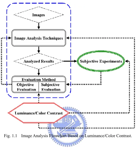
As shown in Fig. 1.1, the block diagram within the blue contour shows a conventional flowchart for an image analysis system. In this flowchart, four essential steps are included: 1) inputting of images to be analyzed, 2) image analysis with one or more techniques, 3) outputting of analyzed results, and 4) evaluation of the analyzed results. Specifically, given one or more images to be analyzed, different image analysis techniques are adopted for different applications. The analyzed results are then evaluated with some evaluation methods according to predefined visual perception requirements. Especially, the evaluation methods could be further categorized into 1) objective evaluation methods and 2) subjective evaluation methods.

and 2) measurement of luminance/color contrast and/or measurement of visual perception quantities. To mimic the way humans perform image analysis, we need some suitable subjective visual quantities. For example, in color segmentation applications, subjective visual quantities such as the degree of segmentation quality, the degree of over-segmentation, and the degree of under-segmentation may be considered to be essential. To extract appropriate visual quantities that may well correspond to humans’ perception, subjective experiments are necessary. Moreover, subjective experiments may also be useful in discovering the relationships among these selected visual quantities.

On the other hand, to measure these visual quantities for a specific application, we need to propose effective and efficient objective quantitative measures. In this dissertation, we consider the use of luminance/color contrast-based measures to mimic the way humans perform image analysis. In fact, in our study, the luminance/color contrast is used in the blocks of image analysis, evaluation methods, and subjective experiments in Fig. 1.1. For example, in the development of color segmentation algorithms, with proper definitions of color contrast in terms of color difference, we demand that pixels with invisible color difference are to be merged together, while pixels with visible color difference are treated as edges. Based on the visible color difference, some quantitative measures are proposed as the objective counterparts of the subjective visual quantities, which are considered in the subjective experiments. Based on the subjective experiments, the correlations between the subjective visual quantities and the objective quantitative measures are verified. Then, these objective measures can be used for the development of evaluation methods for color segmentation and/or for the development of color segmentation algorithms.

Fig. 1.1 Image Analysis Flowchart Based on Luminance/Color Contrast.

Fig. 1.2 and Fig. 1.3 show two examples for image analysis applications. Fig. 1.2 shows the illustration of a luminance contrast-based auto-inspection process for the detection of visual defects on LCD panels. On the other hand, Fig. 1.3 shows the illustration of a color contrast-based color segmentation process.

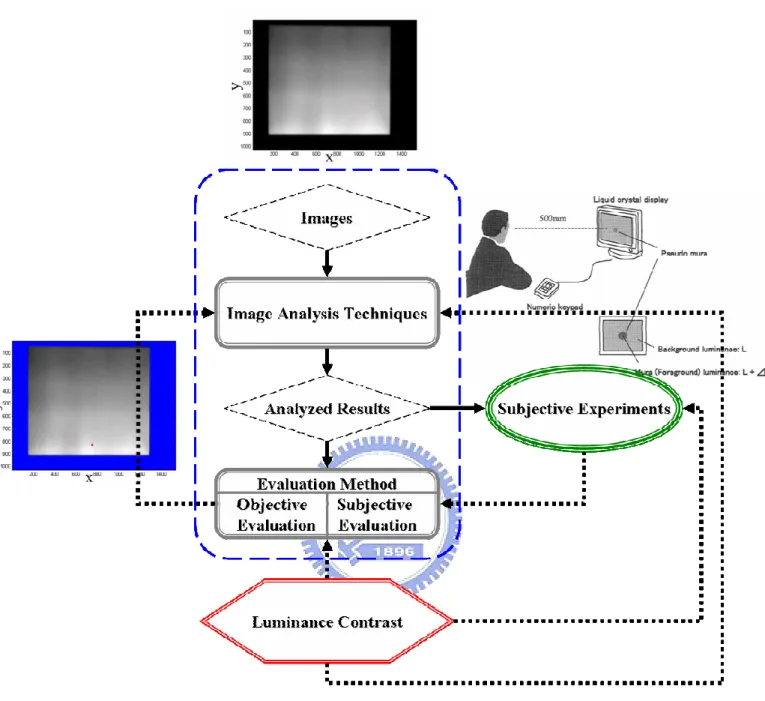
Fig. 1.2 Automatic Inspection Based on Luminance Contrast.

The gray-level image at the top of Fig. 1.2 represents the image of an LCD panel. Compared to a uniform background, the areas with noticeable luminance difference are considered as defects in human’s perception. To mimic the way human detects these defects, some luminance contrast-based visual perception formulas, like the SEMU formula explored by Mori et al, can be deduced based on properly designed subjective experiments, as illustrated in the right side of Fig. 1.2. With this SEMU

formula, we develop an optimal threshold mechanism unified with some specified analysis techniques, as explained in Chapter 3 of this dissertation. The analyzed result is then shown in the left side of Fig. 1.2, where the red point indicates a detected Cluster Mura with a very low luminance contrast.

Fig. 1.3 Color Segmentation Based on Color Contrast.

On the other hand, Fig. 1.3 shows the illustration for color segmentation application. The top image shows the input image to be processed. To avoid directly measuring the subjective quality of color segmentation, two subjective visual

quantities, the quantity of missing boundaries and the quantity of fake boundaries, are considered in this dissertation. As shown in the right side of Fig. 1.3, a few subjective experiments are performed to verify the correlations between these two visual quantities and the quality of color segmentation. On the other hand, an objective quantity, named visible color difference, is defined. Intuitively, given a color image, adjacent pixels with invisible color difference are considered to be grouped together, while adjacent pixels with visible color difference are regarded as image edges. Hence, based on the visible color difference, some objective visual quantities, such as the “intra region visual error measure” and the “inter region visual error measure”, are proposed to measure the degree of missing boundaries and the degree of fake boundaries. With the subjective experiments, the correlations between the subjective visual quantities and the objective quantitative measures can be verified. With these objective visual quantities, we may propose image analysis techniques for color segmentation and the evaluation color segmentation. For example, in the left side of Fig. 1.3, an image in pseudo colors indicates such a segmented result based on the developed color segmentation algorithm. In this image, pixels painted with the same color are segmented into the same region.

1.2

Organization and Contribution

The following chapters in this dissertation are organized as follows.

‹ In Chapter 2, some definitions of luminance/color contrast for different image analysis applications are introduced. Also, for the color segmentation issue, some existing image segmentation algorithms and evaluation methods in the literature are introduced.

‹ In Chapter 3, for the automatic inspection of defects on LCDs, a luminance contrast based formula, named SEMU formula, is introduced. A SEMU-based optimal thresholding mechanism is then proposed to automatically inspect Cluster defects on LCDs.

‹ In Section 4.1, the definition of a directional color contrast is proposed first. Then, with the directional color contrast, the definition of color contrast in the CIE L*a*b* color space is proposed. Also, a technique that can estimate the directional color contrast of color edges in a color image is proposed. On the other hand, a definition of “visible color difference” in the CIE L*a*b* color space is introduced to represent the effects of color difference in human visual perception. Then, based the defined color contrast, a so-called visible color difference is proposed to differentiate visible color difference from invisible color difference. In Section 4.2, some visual rating experiments are performed to verify the correlation between segmentation quality and degree of over-segmentation and/or degree of under-segmentation. Then, based on the defined “visible color difference” formula in Section 4.1, which are used to estimate the degree of over-segmentation, the degree of under-segmentation, and segmentation quality, some quantitative visual error measures are proposed. These quantitative measures are also used in the evaluation of color

segmentation. In Section 4.3, based on the directional color contrast introduced in Section 4.1, a color segmentation algorithm is proposed. On the other hand, uniting with the proposed quantitative evaluation method mentioned in Section 4.2, a new color segmentation algorithm is proposed.

CHAPTER 2

Backgrounds

______________________________________________

Luminance/color contrast has played an important role in the development of image analysis techniques. In Section 2.1, some existing definitions of luminance/color contrast for different applications will be introduced first. On the other hand, since in this dissertation the evaluation of image segmentation results is especially discussed, the backgrounds for image segmentation algorithms and related evaluation methods are briefly introduced in Section 2.2.

2.1

Luminance/Color Contrast

To measure luminance/color contrast, several definitions of luminance/color contrast have already been proposed for various applications. In Section 2.1.1, we first introduce some existing definitions of luminance contrast. Then, in Section 2.1.2, among a variety of color difference definitions, we introduce the CIE L*a*b* color difference. Based on the CIE L*a*b* color difference, we will propose in the following chapters a few more definitions about color difference.

2.1.1 Luminance Contrast

In this section, we introduce four commonly used definitions related to luminance contrast: 1) Luminance Contrast (Weber Contrast), 2) Luminance Ratio, 3) Peak-to-Peak Contrast (Michelson Contrast, Modulation), and 4) Just Noticeable Difference (JND). The details for each of these four definitions are as follows.

1) Luminance Contrast, or Weber Contrast:

To define the relationship between the luminance of an interested area and the luminance of the surrounding area, a measure called Weber contrast is defined in [1]:

CW = (LS–Lb) / Lb. (2.1)

Here, LS is the luminance of the interested area and Lb is the luminance of the

adjacent background. In [1], a thorough technical discussion of this type of measure can be found.

When the background is brighter than the interested area, CW is negative and

ranges from zero to –1. On the contrary, when the background is darker, CW is a

positive number that can be potentially very large. Hence, the sign and value of Cw can be used to describe the relationship between the luminance of an interested area and the luminance of the adjacent background.

2) Luminance Ratio:

To specify the difference between bright parts and dark parts in a photo, another measure called Contrast Ratio is often used. This contrast ratio is defined as:

CR = LS / Lb. (2.2)

In practice, a logarithmic variation of this CR definition, as expressed in (2.3), is also widely used.

log(CR) = log(LS) – log(Lb). (2.3)

In Equation (2.2), the contrast ratio is defined as LS divided by Lb, where LS and

Lb have the same definitions as that in (2.1). The Lb in the denominator is often a

reasonable estimate of the adapted luminance level around this stimulus level in human eyes. Instead of the luminance difference away from the background, the numerator is defined as the luminance of the interested area, Hence, this CR definition has a rather different mathematical behavior from the Weber contrast.

3) Peak-to-Peak Contrast (Michelson Contrast, Modulation):

To determine the strength of a signal luminance relative to the noise luminance level [1], a measure which evaluates the relation between the spread and the sum of signal and noise is introduced. Here, we have

Modulation = (Lmax - Lmin) / (Lmax + Lmin) (2.4)

In the context of human vision, such kind of noise fluctuation could be caused by scattered lights introduced into the view path by a translucent element, which partly obscures the scene behind it.

4) JND (Abbreviation for Just Noticeable Difference) [2]:

For a certain stimulus, the smallest change in the stimulus that can be perceived by human is called the JND. The JND measure is usually used in the study of Psychophysics. Specifically, this definition is often used to indicate a measure in the statistical sense that the probability of being “perceptible” is 50%. For different applications, the definition of the JND measure could be different. Especially in the FPD (Flat Panel Display) visual inspection problem that is to be discussed in this dissertation, the JND over a uniform luminance background is regarded as a gauge of luminance contrast.

2.1.2 CIE L*a*b* Color Difference

On the other hand, for color images, color difference is usually adopted as a gauge of color contrast. Among a variety of color difference definitions, we focus on the CIE L*a*b* color difference. In Section 2.1.2.1, the CIE L*a*b* color space is to be introduced. The color space transformation from the RGB color space to the CIE L*a*b* color space is also described. Then, in Section 2.1.2.2, we introduce the definition of color difference in this CIE L*a*b* color space.

2.1.2.1 CIE L*a*b* Color Space

In the analysis of colors, a proper choice of the color space is a key issue. In this dissertation, we demand three major requirements in the selection of color space: 1) separation of achromatic information from chromatic information, 2) uniform color space, and 3) similar to human visual perception. Among various color spaces, we pick the CIE L*a*b* color space. In this color space, L* represents luminance, while a* and b* represent color components. The definitions for L*, a*, and b* are expressed as follows.

, * 116 _−16            × = n Y Y f L (2.5) , 500 * _            −       × = n n Y Y f X X f a (2.6) , 200 * _            −       × = n n Z Z f Y Y f b (2.7)        ≤ +       × =       >       =       ; . , . ; . , / 008856 0 for 116 16 787 7 008856 0 for 3 1 n n n n n n Y Y Y Y Y Y f Y Y Y Y Y Y f (2.8) ) , _n n n Y Z X , ( : Reference white

The detail about the CIE L*a*b* space can be easily found in many color related books, like [6]. In Figure 2.1, we show an illustration of this CIE L*a*b* color space.

Fig. 2.1 Illustration of the CIE L*a*b* color space [7].

On the other hand, Fig. 2.2 illustrates the color transformation from the CIE L*a*b* color space to the RGB color space. To digitize colors in photos, the (L*,a*,b*) values within an area of interest are first converted to (Rt, Gt, Bt) by using Equations

          ⋅           =           t t t B G R C C C C C C C C C Z Y X 33 32 31 23 22 21 13 12 11 (2.9)

In (2.9), Rt, Gt, and Bt are stimulus values captured from the scenery. C11, C12, …, C33

are the coefficients of the color transformation from the RGB color space to the XYZ color space. Convert (L*,a*,b*) to (R_t,G_t,B_t) Gamma Correction Gamma Correction γ 1 I I

Storage

_Monitor

Y

α

Y

Camera

(R, G, B) (L*,a*,b*) Color Space Conversion Nonlinear Effect Nonlinear Effect Convert (L*,a*,b*) to (R_t,G_t,B_t) Gamma Correction Gamma Correction γ 1 I I γ 1 I I

Storage

_Monitor

Y

α

Y

Y

α

Y

Camera

(R, G, B) (R, G, B) (L*,a*,b*) Color Space Conversion Nonlinear Effect Nonlinear Effect

Fig. 2.2 Color space transformation from the CIE L*a*b* space to the RGB color space.

Then, for the compression of data size and the compensation of the nonlinear effect of the monitors, the (Rt, Gt, Bt) values are further mapped to the (R, G, B) values by

applying the Gamma correction process expressed in Equation (2.10).

) , , ( ) , , (R G B R R G G B B t t t γ γ γ = . (2.10) In Equation (2.10), γ_R,γ_G,γ_B indicate the nonlinear gamma factors for the R, G, and G channels of the output monitor.

2.1.2.2 Color Difference in CIE L*a*b* Color Space

In the CIE L*a*b* space, the differences of color components between Patch X and Patch Y are defined by their differences in lightness (∆L*_{), redness-greenness (∆a}*_),

and yellowness-blueness (∆b*_{). That is,}

* * * Y X L L L = − ∆ (2.11) * * * Y X a a a = − ∆ (2.12) * * * Y X b b b = − ∆ (2.13) The overall color difference between these two samples is defined as the Euclidean distance in the CIE L*a*b*. That is,

2 / 1 * * 2 * * _{[( L) ( a ) ( b )]} E_ab= ∆ + ∆ + ∆ ∆ (2.14) The differences in color can also be defined by the differences in lightness (∆L*_),

chroma ( * ab C ∆ ), and hue ( * ab H ∆ ) [8]. In mathematics, we have * * * B A L L L = − ∆ (2.15) * ₍ *2 *2₎1/2 ₍ *2 *2₎1/2 B B A A ab a b a b C = + − + ∆ (2.16) 2 / 1 2 * 2 * 2 * * _{[( ) ( ) ( ) ]} ab ab ab E L C H = ∆ − ∆ − ∆ ∆ (2.17) or 2 / 1 * * 2 * * _{[( ) ( ) ( )]} ab ab ab L C H E = ∆ + ∆ + ∆ ∆ . (2.18)

2.2

Introduction of Image Segmentation

In Section 2.2.1, we will introduce some existing image segmentation algorithms first. Then, evaluation methods for color segmentation are introduced in Section 2.2.2.

2.2.1 Image Segmentation Algorithms

In recent years, plenty of efforts have been focusing on the segmentation of color images. In general, current image segmentation algorithms can be roughly classified into three major categories: 1) image domain-based techniques; 2) feature space-based techniques; and 3) physics-based techniques [13]. For image domain-based techniques, like [14], the similarity of neighboring pixels or the discontinuity of local information is used as the gauge for segmentation. Adjacent pixels with small intensity/color variations are merged together, while pixels with large enough variations are split apart. For feature space-based techniques, like [26], the data distribution of the entire image plays a crucial role. Clustering or grouping techniques are usually applied over the data distribution to allot image data into groups. On the other hand, for physics-based techniques, the adopted mathematical tools are basically the same as the former two kinds of techniques, while an underlying physical model is used to account for the reflection properties of colored matter [40].

2.2.1.1 Image Domain-Based Approaches

In general, for image domain-based techniques, the similarity of neighboring pixels or the discontinuity of local information is used as the gauge for segmentation. These image domain-based methods could be roughly classified into two kinds of methods: 1) edge-based methods and 2) region-based methods. Edge-based methods usually split apart pixels with large enough data variations, while region-based methods

merge together adjacent pixels with small intensity/color variations.

2.2.1.1.1 Edge-Based Methods

As mentioned above, edge-based methods usually split apart pixels with large enough data variations. So far, plentiful methods have been proposed to detect image boundaries/edges. For example, in [16], to detect boundaries in a given image, three criteria are introduced by the author: 1) good detection, 2) good localization, and 3) single response to a single edge. To have good boundary detection, the detector maximizes the signal-to-noise ratio; on the other hand, to have good localization of boundaries, the detected edge points should be as close to the position of the true edge as possible. With these three criteria, the author finds the optimal detector based on numerical optimization. In [14] and [18], the authors proposed a boundary detection scheme based on “edge flow”. This scheme utilizes a predictive coding model to identify the direction of change in colors and textures at each image location at a given scale. An edge flow vector at each image location is then constructed. By propagating the edge flow vectors, the boundaries can be detected at the image locations where two opposite directions of flow are encountered in a stable state. On the other hand, in [17] and [19], the gradient vector of intensity/color data is used as a gauge to locate boundaries. Usually, the locations with large gradient values are regarded as the locations of edges.

2.2.1.1.2 Region-Based Methods

Different from edge-based methods, region-based methods merge adjacent pixels with small intensity/color variations into regions. In [15] and [23], colors in an image are first quantized into several representative classes. These image pixels are then replaced by the corresponding color-class labels. Then, a criterion using the class-map

is proposed to estimate the data variations in local windows. A region growing method is used to segment the image based on the estimated data variations. In [20][21][22][25], image gradient is used as a gauge to estimate image boundaries/edges. By applying the watershed transform on the gradient magnitude, primitive regions can be produced. Then, region competition, region growing, and/or region merging are used to produce the final segmentation results.

2.2.1.2 Feature Space-Based Approaches

For feature space-based techniques [26], the data distribution of the entire image plays a crucial role. Clustering or grouping techniques are usually applied over the data distribution to allot image data into groups. In [26] and [33], given a color image, a neighborhood is modeled as a distribution of colors. Then, the authors tried to show that the increase in the accuracy of the representation causes higher-quality results for low-level vision tasks on complicated natural images, especially as the size neighborhood increases. In [27][30][32], the authors proposed a general non-parametric technique to analyze a complex multimodal feature space and to delineate arbitrarily shaped clusters in the feature space. A recursive mean shift procedure is used to detect the modes of the distribution. Based on the estimated modes of the distribution, an image segmentation algorithm is performed by classifying images pixels into corresponding clusters. On the other hand, in [29] and [34], the authors treated image segmentation as a graph partitioning problem and proposed a so-called “normalized cut” method to segment the graph. The normalized cut method measures the overall dissimilarity between different groups as well as the overall similarity within the groups. In [31], image segmentation is formulated as a data clustering problem based sparse proximity data. Dissimilarities of pairs of textured regions are computed based on a multiscale Gabor filter representation. Then,

an optimization framework, which uses statistical tests as a measure of homogeneity, is proposed for unsupervised texture segmentation. In [35], the authors extended the general idea of a histogram to the homogeneity domain. Then, uniform regions are identified via multi-level thresholding on the homogeneity histogram. On the other hand, in [36][37][38], based on statistical frameworks with the assumption of Gaussian/Non-Gaussian densities, image analysis techniques, such as expectation maximization, independent component analysis, or Data-Driven Markov Chain Monte Carlo, are applied for image segmentation.

2.2.1.3 Physics-Based Approaches

For physics-based techniques, the adopted mathematical tools are basically the same as the former two kinds of techniques, while an underlying physical model is used to account for the reflection properties of colored matter [40]. In [13] and [40], several photometric invariant similarity measures are proposed to assist image analysis techniques in handling undesired imaging conditions, such as shading, shadows, illumination changes, and highlights.

2.2.2 Evaluation Methods for Image Segmentation

Color segmentation is a crucial step in image analysis and pattern recognition. The performance of color segmentation may significantly affect the quality of an image understanding system. So far, hundreds of color segmentation algorithms have already been developed to deal with various kinds of image-related applications [13][41]. For these color segmentation algorithms, the automatic setting of controlling parameters is usually a difficult task. Currently, these control parameters are often adjusted by the users in an interactive and tiresome manner. Moreover, the selection of control parameters is also image-dependent. For most color segmentation algorithms, there exists no parameter setting that is universally applicable.

On the other hand, it is well known that performance evaluation of segmentation algorithms is critical and essential in the development of image understanding systems. However, as compared with the tremendous efforts spent in the development of segmentation algorithms, relatively fewer efforts have been made on the subject of image segmentation evaluation [42][43][44][45][46]. As shown in Fig. 2.3, Zhang classified existing evaluation methods for image segmentation into three categories [42][43]: 1) analytical methods; 2) discrepancy methods; and 3) goodness methods. Analytical methods directly evaluate segmentation algorithms by analyzing their principles, requirements, utilities and complexity, etc [42][43]. Due to the lack of a general theory for image segmentation, analytical methods work well only for some particular models or for some desirable properties of the algorithms. Moreover, these analytical methods themselves are seldom used alone. On the contrary, both discrepancy methods and goodness methods evaluate the performance of segmentation by judging the quality of segmentation results directly. Especially, discrepancy methods measure the difference between the segmentation result and a

reference result, which is usually an expected result or a ground truth [47][48]. On the other hand, as illustrated in Fig. 2.3, goodness methods evaluate the segmentation results directly with certain quality measures, without the use of any reference result.

Fig. 2.3 Approaches for Evaluating Image Segmentation [42][43].

Among these three evaluation categories, the third type of methods, the goodness methods, is considered a more practical approach due to its direct evaluation of segmentation results without any user-dependent ground truth [49][50]. In this dissertation, we’ll focus on this type of evaluation methods. Moreover, we believe that, some evaluation principles and formulas in these evaluation methods can be used to facilitate the development of segmentation algorithm. Hence, some goodness measures that had been proposed before are to be used in the development of a segmentation algorithm in this dissertation.

So far, several goodness methods have already been proposed [42][43][49][50]. One type of method is to evaluate segmented results with the use of the “Peak Signal to Noise Ratio” (PSNR) function, which is defined as follows:

( )

_{( )}

_      = I MSE f PSNR 2 10 255 10 log , and (2.19)

( )

_{∑ ∑}

(

(

)

(

)

) (

)

= = × − = N x M y M N y x f y x f f MSE 1 1 2 , ' , , (2.20)

where I is an N×M color image f(x,y), and f’(x,y) is denoted as the segmented result, with the color of each segmented region being filled with the average color of that region. Then, with a specified region number, the desired segmented results are defined to be the results with the maximal PSNR value, or equally with the minimum MSE value. In general, this type of method tends to measure the within-region color difference between the original color image and the segmented result. However, due to the lack of consideration regarding the color contrast between adjacent regions, this type of method tends to prefer over-segmented results, which include many small regions. This is because a larger value of MSE would be expected when we merge several small regions into a large one.

To avoid producing overly segmented results, the factor of region area is considered in the approach proposed by Liu and Yang [49]. In their approach, an evaluation function named F function is defined as:

( )

₍

₎

_∑

= × × = R i _i i A e R M N I F 1 2 1000 1 , (2.21)

where I is the image to be segmented, R is the number of regions in the segmented image, ei is the color error of the ith region, Ai is the area of the ith region, and N, M

represent the length and width of the image. Here, ei is defined as the sum of the

Euclidean distance in the RGB color space between the color vectors in the original image and the color vectors in the segmented image, in the ith region. Consequently, with a smaller F-function value, the segmented result is regarded to be better.

segmented results from including too many small regions, the relation between color difference and region area is not clearly treated. Hence, these F-function based methods may include both over-segmented regions and under-segmented regions at the same time. Furthermore, since these evaluation functions only consider the color differences within regions but ignore the color contrast between regions, they may cause some undesired circumstances. For example, the segmented result with each pixel being labeled as an independent region may be treated as a “perfect” result without any color difference error.

Based on Equation (2.21), two further improved evaluation functions are proposed in [50] that are defined as:

( )

₍

₎

_∑

[

( )

]

_∑

= + = × × × = ′ R i _i i A Max A A e A R M N I F 1 2 1 1 1 10000 1 / _{, (2.22)} and

( )

₍

₎

_∑

( )

=               + + × × × = R i i i i i A A R A e R M N I Q 1 2 2 1 10000 1 log , (2.23)

where R(Ai) represents the number of regions with the area size Ai. In both equations,

the areas of regions are considered to punish these segmentation results with too many small regions. Similarly, the number of segmented regions is also included, aiming to achieve segmented results with an appropriate number of homogeneous regions.

For the above evaluation functions, two primary requirements are adopted to define “preferred” segmentation results: smaller color difference and fewer segmented regions. However, color difference and the number of segmented regions are two very different measures in their physical meanings. The trade-off between these two measures would be very difficult. Moreover, the preferred number of segmented regions could be very different from image to image. When this image-dependent measure is involved in a single evaluation function, it would be rather difficult to

perform segmentation evaluation without having the prior knowledge of the image contents in advance.

In summary, although several goodness functions have already been proposed, most of them are not directly based on human visual perception. Instead, most goodness methods combine several existing measures together to formulate their evaluation functions. The selection and combination of measures are usually subjective. The adjustment of weighting coefficients is often troublesome. Moreover, for most evaluation methods, the quality of segmentation is usually represented in a single function, which mixes together several weakly related measures. Without knowing the erroneous information about the segmented result under evaluation, these approaches could be very unreliable.

CHAPTER 3

Visual Inspection for Mura on LCDs

Based on Luminance Contrast

______________________________________________

3.1

Introduction of Automatic Inspection for

Mura on LCDs

Recently, Liquid Crystal Displays (LCDs) have received increasing market attention because of the decreasing prices and the improved visual quality. Among several characteristics regarding the visual quality of LCDs, the front-of-screen (FOS) quality of LCDs is essential. Most existing FOS quality tests depend on the perception of human eyes. However, human inspection needs higher labor power and usually causes inefficient and inconsistent inspection. Instead of human inspection, automatic inspection that employs efficient algorithms over photographed images could be a reasonable and reliable way to evaluate the FOS quality of LCDs.

and the establishment of quality evaluation standards [2][9]. For example, the Video Electronics Standards Association (VESA) has been carrying activities related to the standards for classifying defects [9], and the Semiconductor Equipment and Materials International (SEMI) has spent a lot of efforts on the standardization of defect quantification [2]. However, even though there is a high demand of automatic inspection of FOS quality, there are relatively few efforts spent on the development of defect detection algorithms [3][10][11][12].

Fig. 3.1 Cross-section of an active matrix TFT-LCD.

In this chapter, we focus on the development of detection algorithms for the inspection of the FOS quality of an active matrix thin-film transistor liquid crystal display (AM TFT-LCD). Fig. 3.1 illustrates the cross-section of an AM TFT-LCD. Basically, an LCD display includes two essential components: Cell Unit and Backlight Unit. In the cell unit, there are mainly five elements: liquid crystal, thin-film-transistor (TFT) array, color filters, glasses, and polarizer. In general, the functionality of cell unit is to make the RGB color switching at each pixel controllable. On the other hand, in the backlight unit, there are four basic elements: lamp, light pipe,

reflective film and optical film. Generally, the functionality of backlight unit is to produce uniform light.

In the inspection of FOS quality, the so-called Mura defects greatly influence the FOS quality [9]. The Mura defects are defined as the visible imperfections of the FOS of a display screen in active use. Mura defects usually appear as a low contrast, non-uniform brightness regions, typically larger than a single pixel [2]. As shown in Table 3.1 Mori et al [10] listed several causes of Mura defects in TFT-LCD. Usually, the manufacturing performance of each component in the cell unit or in the backlight unit would affect the appearance of Mura defects. A superior manufacture process produces fewer Mura defects. Usually, the non-uniformity in various kinds of components induces different kinds of Mura defects.

Table 3.1 Causes of Mura defects on TFT-LCD [10]

Basic Unit Causes of Mura

(1) Non-uniform gap between glasses (2) Non-uniform color of color filter (3) Non-uniform density of liquid crystal Cell unit

(4) Non-uniform thickness of TFT array layer (5) Wrinkled optical filter

3.1.1 SEMU Formula Based on Just Noticeable Difference

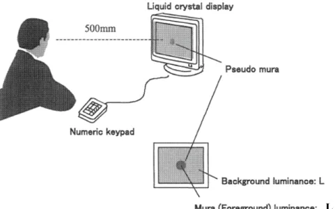
As mentioned above, Mura indicates the defects as the visible imperfections on the FOS of a display screen. To make standard for the quantification of Mura phenomenon, a committee in SEMI defines a measurement index for Mura in the inspection of FPD (Flat Panel Display) image quality. To define Mura, an ergonomic approach is used to investigate human eye’s sensitivity with respect to Mura by exploring the relation between Mura’s area and contrast. Also, an index, named SEMU (Semi Mura), is defined to express the degree of Mura defects. This SEMU index is defined to be the ratio of the target’s contrast over the contrast at JND. To deduce the SEMU formula, a subjective experiment had been conducted in [3], as shown in Fig. 3.2. In this experiment, a special LCD panel was produced to display 256 gradations in the luminance range between 43 cd/m2 and 54 cd/m2. A program created synthesized Mura and displayed the Mura at the center of the LCD panel. The observer looked at the screen with both eyes without any artificial pupil. The viewing direction is normal to the center of the LCD panel and the viewing distance is 500 mm. The experiments were performed in a darkroom and the observer could freely adjust the luminance of the displayed Mura by using a numeric keypad. The test began with the gray level of the synthesized Mura set to the same level as that of the background. Then, the observer adjusted the luminance of the Mura to the level where the Mura region was just perceptible and also to another level where the Mura can be clearly detected. The contrast values of the synthesized Mura at both levels were recorded. The contrast at the first level provided the data for the JND (Just Noticeable Difference) contrast, while the contrast at the second level provided the data for the “Dist (Distinct difference)” contrast.

L + ∆L

L + ∆L

Fig. 3.2 Experimental conditions and equipment used in the subjective evaluations in [3].

Assume the background luminance is denoted as L and the Mura luminance is denoted as L + ∆L. In this experiment, the contrast of the Mura was defined to be the value of ∆L/L. Various sizes of circle-type and rectangle-type Muras were used in the experiments. The observers include 8 experts, who regularly conduct Mura inspections and analysis, and 8 college students with normal vision (with near vision strength (500mm) of 1.2 or greater for both eyes).

Fig. 3.3 shows the experimental results for Muras larger than 1 pixel, where the horizontal axis is 1/A0.33 and the vertical axis is the value of contrast. The observers’ JND data are plotted as “ •”, while the Dist data are plotted as “ο”. The bold line was determined by the linear regression of the JND data. This line indicates a strong correlation between the size of Mura and the perceived contrast value of Mura. In this experiment, the larger the area of the Mura is, the smaller the JND contrast becomes. In other words, Muras are more visible as their area becomes larger. In mathematics, the linear relationship between JND contrast (Cjnd) and A0.33 was expressed in [3] as

Cjnd = 1.97/A0.33 + 0.72. (3.1)

difference” for LCD Muras.

Fig. 3.3 JND and Dist result of the subjective evaluation in [3]. f(A) = A0.33, A: Mura area (mm2)

Fig. 3.3 also shows the straight lines for 2.0×Cjnd and 3.0×Cjnd. The Dist contrast data is around the 2.0×Cjnd line. This indicates that not only the JND level but also the visible contrast level has the linear relationship between the contrast level and A0.33. Hence, the level of Mura defects can be described accordingly.

To evaluate the blemish degree of Cluster Mura defect, the SEMU formula is defined as: ) . . (197_0.33 +072 = ≡ A C C C SEMU x jnd x , (3.2)

where Cx is the average contrast of Mura, Cjnd is the just noticeable contrast of Mura,

blemish. In [4] and [5], some modified versions of this SEMU formula have been further proposed. In these modified SEMU formulae, the contrast and the area of Mura defects are still the main factors. Similar to Equation (3.2), either a larger contrast of Mura or a larger area of Mura will cause a higher degree of blemish.

As mentioned above, Mura defects appear as low contrast, non-uniform brightness regions. They are typically larger than a single pixel when the screen is at a constant gray level. Moreover, various kinds of Mura defects are caused by different reasons. It would be difficult to develop a single universal algorithm to detect all kinds of Mura defects. In this dissertation, we consider two major kinds of Mura defects, Cluster Mura and Vertical-Band Mura. These two types of Mura are common in the FOS of LCDs. In Section 3.2, we’ll introduce the photography of the FOS image first. Then, in Section 3.3, the proposed techniques in the detection of Cluster Mura are discussed. In Section 3.4, on the other hand, we discuss the proposed techniques for the detection of Vertical-Band Mura.

3.2

Photography of FOS Images

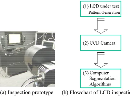
Fig. 3.4(a) shows the prototype of our automatic inspection system. In this system, we have an LCD panel that is under test, a CCD camera to capture the FOS image of the LCD panel, and a computer to execute Mura detection algorithms. In the inspection process, the LCD panel under test is vertically placed on the apparatus. Each time, the LCD panel is driven by a pattern generator to display a certain gray level image pattern. Then, the camera will capture an FOS image for this specific pattern. The FOS image is transmitted to the computer for storage and then is inspected by a set of Mura detection algorithms.

At markets, 15-inch and 17-inch LCD panels are the mainstream for desktop displays and notebook displays. In fact, the manufacture processes in these two types of LCD panels are quite similar. Hence, the appearances of Mura defects are also similar. Both types of LCD panels can be inspected by this prototype system. Moreover, to mimic the performance of human inspection, the specifications of the CCD camera are chosen to have a more than 12-bit dynamic range and a spatial resolution of 1532 × 1024 pixels.

(a) Inspection prototype (b) Flowchart of LCD inspection Fig. 3.4 The prototype of the LCD inspection system.

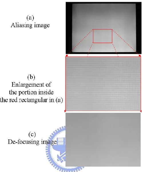
3.2.1 Aliasing

In the photography process, aliasing usually occurs when the lens of camera is well focused on the center of the FOS. Fig. 3.5(a) shows an image with aliasing. Fig. 3.5(b) shows the enlarged image of the portion inside the red rectangular in Fig. 3.5(a). As shown in Fig. 3.5(b), the lattice-like pattern occurs when the camera lens is in focus. This lattice-like pattern will not only increase the difficulty in automatic inspection but also influence the inspection results of Mura defects.

To eliminate the aliasing effect, several anti-aliasing approaches have already been published or patented [51][52]. These approaches usually require additional accessories and may cause image blurring. Among these approaches, we adopt the de-focusing approach, which may eliminate the aliasing effect without additional accessories. In this approach, we focus the camera lens on the FOS of LCD first, followed by slightly de-focusing the lens till the lattice-like pattern disappears. Although this method still causes some degree of blurring in the FOS image, this method demands no extra expense. In Fig. 3.5(c), we show the de-focused image of Fig. 3.5(a). It can be easily seen that the lattice-like pattern is suppressed.

3.2.2 Cluster Mura and V-Band Mura

Among several kinds of Mura defects, the detection of two major kinds of Mura defects, Cluster Mura and Vertical Band (V-Band) Mura, will be taken into account in this dissertation. As mentioned before, Mura defects appear as non-uniform brightness regions in the FOS of an LCD panel. Nevertheless, not all kinds of Mura defects appear in a similar manner. For example, Cluster Mura usually appears as a cluster of several points locating within a small area. As shown in Fig. 3.6(a)(c), a round-type Cluster Mura defect locates at (x=750, y=820), while a rectangular-type Cluster Mura defect appears as a narrow region ranging from (x=200, y=720) to (x=600, y=720). On the other hand, a V-Band Mura usually appears as a wide vertical strip with either brighter or darker brightness with respect to the uniform background. As shown in Fig. 3.6(e), a V-Band Mura is centered around x=850. The cause of V-Band Mura usually comes from non-uniform thickness of components, such as non-uniform thickness of the glasses in the cell unit. In comparison, Cluster Muras usually appear within a local area, while V-Band Muras usually occupy a larger area. The appearance model of a Cluster Mura is quite different from that of a V-Band Mura. It would be impractical to detect both types of Muras based on a single algorithm.

(a) Round-type Cluster Mura (b) Detection result of (a)

(c) Rectangular-type Cluster Mura (d) Detection result of (c)

(e) V-Band Mura

In the following sections, we will present the use of two different approaches to deal with these two kinds of Mura defects. These two different approaches actually share the same kernel: a Laplacian of Gaussian (LOG) filter. This LOG filter, which compares the intensity of the target with the intensity of the surroundings, will be demonstrated to be very useful in the development of Mura detection algorithms. To detect Cluster Mura defects, an approach based on 2-D LOG filters will be presented in Section 3.3. To detect V-Band Mura, on the other hand, an approach based on 1-D LOG filters will be presented in Section 3.4.