以碰撞緩和方法應用於布與剛體互動之模擬

國

立

交

通

大

學

多媒體工程研究所

碩

士

論

文

以碰撞緩和方法應用於布與剛體互動之模擬

An Efficient Scheme for Cloth and Rigid Body Interaction with

Collision Alleviation

研 究 生：鄺著軒

以碰撞緩和方法應用於布與剛體互動之模擬

研究生: 鄺著軒

指導教授

施仁忠 教授

國立交通大學多媒體工程研究所

摘 要

)

An Efficient Scheme for Cloth and Rigid Body

Interaction with Collision Alleviation

Student: Chu-Hsuan Kuang

Advisor: Dr. Zen-Chung Shih

Institute of Multimedia Engineering

National Chiao-Tung University

ABSTRACT

We propose an efficient scheme with collision avoidance and alleviation for cloth and rigid body interaction. In this scheme, we also resolve the penetration of particles on cloth and estimate the contact force explicitly. Our system can provide a smooth, inelastic, stable and visually plausible contact simulation in runtime.

Acknowledgements

First of all, I would like to express my sincere gratitude to my advisor, Pro. Zen-Chung Shih, for his guidance and patience. Without his encouragement, I would not complete this thesis. Thank also to all the members in Computer Graphics and Virtual Reality Laboratory for their reinforcement and suggestion. I especially appreciate the helpful discussion with Yu-Ting Tsai, Jhu Chi and my roommate Yong-Jheng Chen. Thank also to Prof. Jen-Duo Liu for his guidance and enlightenment in the beginning of the study. Moreover, I want to thank to all the people who ever supported me during these days. Finally, I will sincerely dedicate this thesis to my parents.

Contents

Abstract (in Chinese) ... I Abstract (in English)...II Contents ... IV List of Figures... VI Chapter 1 Introduction...1 1.1 Motivation...2 1.2 System Overview...2 1.3 Thesis Organization ...3

Chapter 2 Related Work...4

2.1 Physical Model ...4 2.2 Contact Resolution...5 2.2.1 Penalty-based method ...5 2.2.2 Impulse-based method ...6 2.2.3 Constraint-based method ...6 2.3 Coupling...7 Chapter 3 Background ...8

3.1 Rigid Body and Deformable Body...9

3.2 Collision ... 11

3.3 Contact Resolution...12

Chapter 4 Overview of System ...14

4.1 Rigid Object...14

4.1.1 Data Representation...14

4.1.2 Data Structure for Collision...16

4.2 Cloth Object ...18

Chapter 5 Collision Detection and Response...23

5.1 Collision ...23

5.1.1 Phase 1: Collision Avoidance and Alleviation ...23

5.1.2 Phase 2: Collision Removal and Response ...28

5.2 Contact Force ...32

Chapter 6 Implementation and Result...36

6.1 Implementation ...36

6.2 Result...37

Chapter 7 Conclusion and Future Work ...46

List of Figures

Figure 1.1: Cloth simulation used in animation “Monster Inc.”[6] ...1

Figure 3.1: Simulation pipeline ...8

Figure 3.2:Stanford bunny as a rigid body [27] ...9

Figure 3.3:Cloth model ...10

Figure 4.1: Rigid body with mass center at pv and a force acted on pv ...15 a Figure 4.2: Distance field defined for a sphere...16

Figure 4.3: Distance map in [30] ...17

Figure 4.4: Structural, shearing, bending springs for rectangular cloth...19

Figure 4.5: OpenTissue spring structure ...19

Figure 4.6: Repulsion region for every particle ...21

Figure 4.7: Spring applied while particles move within nominal distance...21

Figure 5.1: Collision sequences for real case...24

Figure 5.2: Problems for discrete time step ...25

Figure 5.3: Problem for drastic collision ...26

Figure 5.4: Inelastic collision between objects with asymmetric mass ...26

Figure 5.5: Rigid object entered repulsion region of a particle ...27

Figure 5.6: Rigid object chasing a particle ...29

Figure 5.7: The gravity to particle is greater than the spring force...30

Figure 5.8: Projection for a penetrated particle ...31

Figure 5.9: Problem for projection ...31

Figure 5.10: Sub-force F is used as contact force ...33

Figure 5.11: Particle and rigid object have same velocity direction ...33

Figure 5.12: Particle and rigid object have opposite velocity direction ...34

Figure 6.1: Summary of the Simulation Algorithm ...37

Figure 6.2: Example for repulsion with large radius ...40

Figure 6.3: With or without repulsion...41

Figure 6.4: Example for a rigid object which cannot be influenced by cloth...42

Figure 6.5: Three estimation of contact force...43

Figure 6.6: Example for rigid body rain (20 objects). ...44

Chapter 1

Introduction

Due to the wide usage in industry, physics-based animation is becoming increasingly popular computer graphic subject in recent years. Over decades of research, plenty of physics-based models were proposed to represent real-world object for various purpose. In engineering simulation such as robotic and solid mechanism, an accurate model based on engineering physics is required. In fashion industry of cloth designing, a visual realistic cloth model based on various material’s behavior and characteristics is applied. In animations industry such as Fig 1.1, visual realistic and computation-time-limited approach is appreciated by animator. Moreover, in game industry, run-time efficiency and plausible simulation are the basic requirements. Its application can be seen everywhere from the most famous game console games to special effect such as water-splashing , skin/muscle-deforming in movies.

1.1 Motivation

Physical contact always plays an important roll in physics engine. The most famous game engines such as UNREAL also integrate physics engine to deal with multi-particle or multi-rigid-object collision. However, cloth object is not popular in game industry not only because of the cost for simulation but also the cost to perform seamless interaction with other object. However, cloth object can provide many interesting effects in games or animations such as a floating cloak worn on a character, a spring bed with kids jumping on it and a basketball net waving after a slam dunk. These effects are not necessarily accurate but plausible and efficient .

However, most of researches resolve contact for rigid body or deformable body individually. Some [7] proposed an interaction between cloth and rigid object but only for a static or pre-animated rigid body. A general constraint-based coupling method for rigid and deformable object is proposed in a technical report [5]. However, the performance may dramatically vary by the integration method applied. While a robust, fast, stable and visual plausible simulation method is always welcomed to game industry even if it is inaccurate and explicit.

1.2 System Overview

In this thesis, a collision detection and response scheme for cloth and rigid object is proposed. The collision scheme is separated into two phases. Before penetration actually happens and when two objects moves extremely close to each

into the rigid body, we simply project it out with collision information and then estimate contact force explicitly. The second phase is somewhat similar to constraint-based method but contact force is explicitly calculated independent to integration method. The independency is important because the accuracy of contact reaction usually requires only visual plausibility but motion of objects and cloth can still be accurate and delicate. Furthermore, due to the explicitness, the computation cost can be largely reduced and it is easy to implement with parallel algorithm. Moreover, this estimation method requires only the change of velocity so that it can be free for penetration information, and this may encourage some collision detection methods such as image-based collision detection with weakness in contact information gathering.

The method proposed in this thesis enables simulation of contact between high resolution cloth and large mount of rigid objects in run-time, and also enables a stable, smooth, large-area, long-time contact with cloth surface and rigid body.

1.3 Thesis Organization

The following chapter is organized as follows. In Chapter 2, we review previous researches on physical model and contact resolution. In Chapter 3, a background for a widely-used simulation pipeline is generally introduced step by step. In Chapter 4, an overview of the physical model used in this thesis is described in detail. Then in Chapter 5, we will describe a collision detection and response scheme for cloth and rigid body and discuss about some drawbacks of traditional methods. The implementation and results will be demonstrated in Chapter 6. And finally conclusion and future work are given in Chapter 6.

Chapter 2

Related Work

A review of previous researches is presented as follows. In section 2.1, there are some researches about basic physical model such as rigid body and deformable cloth. Then in section 2.2, we will state some previous researches about contact resolution. And finally in section 2.3, we will present some coupling methods for rigid body and deformable body.

2.1 Physical Model

Rigid body dynamics had been researched for decades and is widely used nowadays [11][19][10][18][16]. Baraff was the first to systematically treat contact problems [2][3][4].

Deformable body dynamics for computer graphic was pioneered by Terzopoulos [31], and then widely discussed ever since. Provot [25] proposed a mass-spring system which constructs deformable surface as a number of particles. The particles are connected to each other with springs as a rectangle grid in order to model various forces such as tensile, shear and bending force. Spring coefficient can be tuned to

unstructured meshes is proposed in [19]. Pascal V. et al.[23] proposed a more accurate way to represent the bending force since bending spring in original model provides not only bending force but also tensile force.

2.2 Contact Resolution

2.2.1 Penalty-based method

On of the first penalty-based method was proposed by Moore et al. [19]. They model contact forces as spring force in computer animation. In addition to use simple linear spring, they modified the spring constant depends on whether motion is approaching or leaving. The relationship is stated as follows:

kleave =εkapproach, (2.1)

while ε is the elasticity of collision so that ε＝0 as inelastic collision and ε＝1 as perfect elastic collision. Terzopoulos, et al. [31] derived the penalty force from energy potential. _⎟⎟ ⎠ ⎞ ⎜⎜ ⎝ ⎛ = ε depth d c E exp . (2.2) F E ddepth n_⎟⎟n ⎠ ⎞ ⎜ ⎜ ⎝ ⎛ ⋅ ⎟⎟ ⎠ ⎞ ⎜⎜ ⎝ ⎛ − ∇ − = ε ε exp (2.3) Hirota et al. [12][13] integrate penalty force over the intersecting polygon and combined with an implicit finite element method. These methods are easy to formulate but have problems in assigning meaningful spring constant for penalty force. That is, the force may be too stiff for a drastic response or too weak to resolve contact.

2.2.2 Impulse-based method

Impulse-based methods resolve contact between objects by modifying velocity according to collision impulse. Moore et al.[19] extended penalty method with an algebraic collision resolving problem, which is similar to Newton’s collision law, and handles colliding contacts before applying springs. Moore [19] and Hahn [11] both modeld the interaction by integrating contact force over times such as

J = Fdt

∫

while Mirtich [18] model contact force as collision impulse train, i.e., a sum of delta function approximating the corresponding time integral. These methods are easily formulated and under some circumstances they may guarantee the existence of the solution. However, they treat even continuous contact as a type of impact so that static contact such as one object resting on another are modeled as a series of collision impulse in a very high frequency.

2.2.3 Constraint-based method

To handle collision, velocity-based formulation is usually used in constraint-based method. It considers impulse-momentum law at the point of collision. Stewart and Trinkle [28] make an impulse-based method and the method is now known as Stewart’s method. Anitescu and Potra [1] extended the method to guarantee existence of the solution. Then Sauer and Schömer [26] extended with a linearized contact condition. Stewart and Trinkle [29] suggest using contact tracking to avoid the problem of explicitly determining all potential active contact constraint.

2.3 Coupling

Most papers discussing contact problems are limited within single dynamic system. An early technical report [5] proposed a method to couple different mechanics models. The system is a black box system which constraint force is the interface among different models. O’Brian et al. [20] presented a coupling system between different mechanics models in context of active or passive system with constraint force so that a pre-animated basketball locus can be modified by interacting with a net. Constraint-based coupling is shown to be general but the calculation of the constraint force may lead to solving large linear system.

Some researches defined a new model to represent both rigid and deformable object so that contact resolution can be unified. Jansson et al.[17] proposed a mass-spring model for modeling both rigid and deformable objects. A spring is created while particles move within a nominal distance in order to push each other away. This method constructs even simple rigid object with nested and large number of spring connections. Moreover, spring constant assignment remains a problem. Pauly [24] proposed a quasi-rigid object which deforms while contact and preserve their basic shape afterward. Galoppo et al. [30] simulate contact between deformable bodies with high-resolution geometry with Dynamic Deformation Textures which enable a heterogeneous object with different stiffness. However, these models require new definition for object while traditional rigid and mass-spring-based deformable object still widely and efficiently used. And also these methods cannot present a deformable surface such as cloth.

Chapter 3

Background

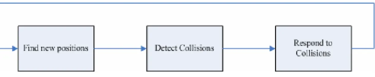
Rather than only moving a single object, interaction among objects makes physics simulation more interesting. During objects moving along, collision occurs. The contact should be detected and then resolved to guarantee no visual penetration since objects do not penetrate each other in reality. In the most popular physics-based simulation pipeline, there are three main simulation steps as described in Fig 3.1. First, move each object with their mechanics. Then trace every object to detect if collision happens. Finally if objects actually contact each other, resolve contact with moderate response.

Figure 3.1: Simulation pipeline

There are two main categories of physical model: rigid body models and deformable body models. Most of time contact issues are discussed individually for different physical models.

3.1 Rigid Body and Deformable Body

Rigid body motion theory is well-established and widely-used today. The main idea is regarding ideal object with stiff and non-deformable material. Due to this assumption, rigid body motion can be simply figured. If a force applied on an object without any deformation, it only changes the velocity of the center of mass, including translation and angular velocity. This property makes motion simulation relatively simple even for complex object. Nevertheless, this also makes contact resolution extra-hard to handle because of the stiffness of rigid body. The reaction produce after collision can be sensitive since collision time is extremely short. Furthermore, most of objects in real world have a little deformation while collision occurs. An famous rigid body model, Stanford bunny, is shown in Fig 3.2.

Figure 3.2:Stanford bunny as a rigid body [27]

Beside rigid body, deformable body which is able to change in geometry is another choice. While there are plenty of models for deformable object, only cloth simulation is discussed in this section because of its special properties.

Cloth is a thin, elastic and highly deformable surface without volume. It moves and deforms according to its structure and the physical laws. Its physically based models can further be classified into two categories: energy-based techniques and

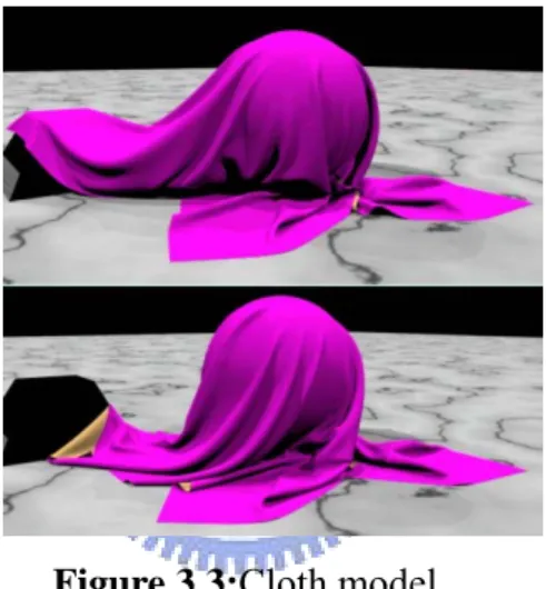
force-based techniques. Energy-based techniques calculate the energy of the whole cloth from a set of equations and determine the shape of the cloth by moving the points to achieve a minimum energy situation, such as Finite Element Method (FEM). Force-based techniques represent the force among points as differential equations and perform a numerical integration to obtain the point positions at each time step, such as mass-spring system. In general energy-based techniques are used to produce static simulation while force-based techniques are used in dynamic simulation. Fig 3.3 shows a cloth model proposed in [7].

Figure 3.3:Cloth model

In most of simulation, objects are usually treated as either rigid or deformable body. In some researches, a semi-deformable object is presented but it requires more complicate representation and may cost more computational time.

3.2 Collision

While most of the physic simulations are not for a single but multiple objects, multi-object interaction is an important issue. During the course of physics-based animation, objects come in contact to each other. The contact should be resolved, either by repulsing or sliding off each other. In order to respond to collision, the collision information such as contact region and contact time is necessary to be gathered. This is the main issue for collision detection. Collision detection can be regarded as a purely geometrical problem.

Many methods are proposed to solve this problem for either rigid body or deformable body. No matter what method is applied, collision detection is often a bottleneck for physic simulation. Hubbard [15] introduced a concept of broad-phase and narrow-phase collision detection. Broad-phase collision detection aims to perform a coarse test which prunes unnecessary test pair to reduce computational cost. And narrow-phase collision detection deals with the actual pair-wise test. For example, broad-phase collision detection methods, such as Bounding Volume Hierarchy and spatial division methods like Octree, KB-Tree, BSP-Tree and spatial hashing method, largely reduce unnecessary testing. And narrow-phase collision detection methods, such as intersection testing between triangles, distance field, layered depth image algorithm, provide actual contact information.

3.3 Contact Resolution

While detecting collision, some useful information such as intersection region and penetration depth can be gathered. With this information, objects can be separated one to another. Basic concept to resolve contact is to change velocity and position of each object, or to apply some force to keep away from each other. There are three main methods to respond to collision: penalty-based method, constraint-based method and impulse-based method.

In real world, rigid bodies do not penetrate each other because contact force will separate them. Penalty-based methods simply treat this force as a spring. Spring system can behavior as a harmonic oscillator under Hooks Law or defined as exponential spring [15]. When collision happens, add a compressed spring between objects and the spring force pushes each object until contact resolved. This method is fast, easy to implement, however, have potential drawback: it is hard to assign physically meaningful spring constant. Moreover, too large constant leads to over reaction while too small constant results in more penetration.

While penalty-based methods apply to deformable unclosed surface such as cloth, penalty force often occurred before contact since cloth does not actually have “inner side”. This penalty method that creates a spring force while two elements are close enough and pushes against each other is often called repulsive force.

Constraint-based methods resolve contact by adding a constraint to move the penetrated objects away. These methods resemble physicists’ view of world. They set

determine the final velocity. That is, the constraint forces the objects changing in position, velocity or force to fulfill the purpose. For example, if two objects penetrated to each other, the velocity each object is then forced to change by constraint in order to separate. The change of velocity implies impulse and contact force which can be solved by a linear equation F_c =KΔv, while K is a square matrix

determined by the different integrator. This method is more physically correct. However, the calculation of contact force requires integration method. The complexity may vary by using different integration method. For example, implicit integration method can be in high dimension for object like cloth.

Impulse-based methods treats even continuous contact as a type of impact

+ ₋ − + − = =

_∫

and use a coefficient of restitution to determine the post-impact velocity of the object [11][19][10][18]. This approach is easier to formulate, but could require a large number of iterations to resolve the resulting impact sequences especially when multipoint collision happens. Although it’s notable for its ability to correctly stops all collisions, but computational cost can be extremely high for multipoint contact. And moreover, it has its own problems when trying to simulate resting contact with complex models and the wobbling problem remains and iteration is generally necessary to remove all collisions.

Chapter 4

Overview of System

Our system couples the main physic-based models: rigid body and cloth. In this chapter, we will discuss about the property of these models in detail. Moreover, we take advantage of some current data structure for collision detection and response in order to facilitate the methods used in next chapter.

4.1 Rigid Object

4.1.1 Data Representation

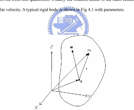
Rigid objects are mostly the simplest model to represent in computer graphic. It can be analyzed with a set of parameters

{

}

object. I is inertia tensor of object, a 3×3 matrix composed of Ixx, Ixy, Ixz, Iyy, Iyz, Izz.

⎥ ⎥ ⎥ ⎦ ⎤ ⎢ ⎢ ⎢ ⎣ ⎡ − − − − − − = zz yz xz yz yy xy xz xy xx I I I I I I I I I I (4.1) Ixx =

∫

∫

I_xy =

∫

I_xz =

∫

I_yz =

∫

For a simple uniformly-dense sphere with radius of r, inertia tensor can be derived as

2 5 2 Mr I I

I_xx= _yy= _zz= and I_xy=I_xz=I_yz=0. pv is the position of the center of mass. vv

is the velocity of the center of mass. O is the orientation of the object along the

rotation center, often represented with quaternion _⎟⎟

⎠ ⎞ ⎜⎜ ⎝ ⎛ ⎟ ⎠ ⎞ ⎜ ⎝ ⎛ ⎟ ⎠ ⎞ ⎜ ⎝ ⎛ u 2 sin , 2 cos θ θ where θ is a

rotation angle and u is a unit length rotation axis, and then a 3×3 rotation matrix can be derived from this quaternion. Usually the rotation center is the mass center. ωv is angular velocity. A typical rigid body is shown in Fig 4.1 with parameters.

Figure 4.1: Rigid body with mass center at pv and a force acted on pv _a

If a force F acts on a rigid object at pv , it can be decomposed into the sub-force a

which acts to center of mass and the sub-force which acts to orientation. That is, force parallels to rˆ , where rˆ is a vector pointing to the center of the mass (i.e.

r r r p p r _{a v} v v v

v_{= − ,ˆ= ), changes the position and velocity of center mass, pv and vv .}

And force perpendicular to rˆ changes the angular velocity and orientation, O and ωv.

( )

dt d I F r _{prependicular} ω τv = v× v = v (4.9) The force can be contact force, constraint force or friction. And by equations (4.7)(4.8)(4.9), the motion of rigid body can be easily computed.

4.1.2 Data Structure for Collision

There are plenty of data structures to solve collision detection problem for rigid body. One of the methods called Distance Field is very suitable for the collision between rigid and deformable-object collision detection and is able to efficiently provide sufficient collision information in run-time.

This method defines space around rigid body with an implicit field function:

R R

D: 3 → so that every point in space is assigned a signed distance value which is

the shortest distance to move inside or outside the object. To illustrate, such field can easily be defined for a spherical object with center of (x, y, z) and radius of R as

( )

(

_p

_x

)

(

_p

_y

)

(

_p

_z

)

−

−

−

where D<0 if p is inside sphere, D>0 if p is outside and D=0 if p is on the surface (Fig 4.2).

Figure 4.3: Distance map in [30]

While most of model are too complicated to represent with a formula, a mapping method called “Distance Map” were proposed. As shown in Fig 4.3, it discretizes space into subspaces and then maps the pre-computed distance value to each subspace unit. Usually space is subdivided into Uniform 3D grids or Octree/ BSP Tree/ KD-Tree for memory-saving purpose. Despite resolution problem, memory cost and pre-computational time, this method is quit suitable for collision detection problem to resolve contact of a particle of deformable object from a rigid object while a particle

can be easily removed from penetration with simply mapping function. And moreover not to mention the benefit from its independently testing with potential to implement in parallelism algorithm that is quit efficient in recent SIMD graphic hardware.

Therefore, a 3D cubic volume texture can represent as a basic bounding volume for rigid object and distance information such as signed distance and normal vector can be stored within texels.

4.2 Cloth Object

4.2.1 Data Representation

There are two main methods to represent a physic model for cloth: discrete model and continuous models. Continuous model method such as finite element method produces an equilibration state for cloth by minimizing energy for every element. This method requires solving non-linear system with large computational time so that is not suited for time-critical runtime simulation but actually able to produces accurate physical model. As long as we require efficiency, a discrete model, mass-spring system, is adopted.

Mass-spring system analyzes physics of cloth as a number of mass particles connected with springs so that springs keep particle moving limitedly under cloth’s original structure from dispersion. Provot [25] proposed a mass-spring system for textiles using a rectangular mesh in which particles are connected with structural springs, diagonal springs and interleaving springs.

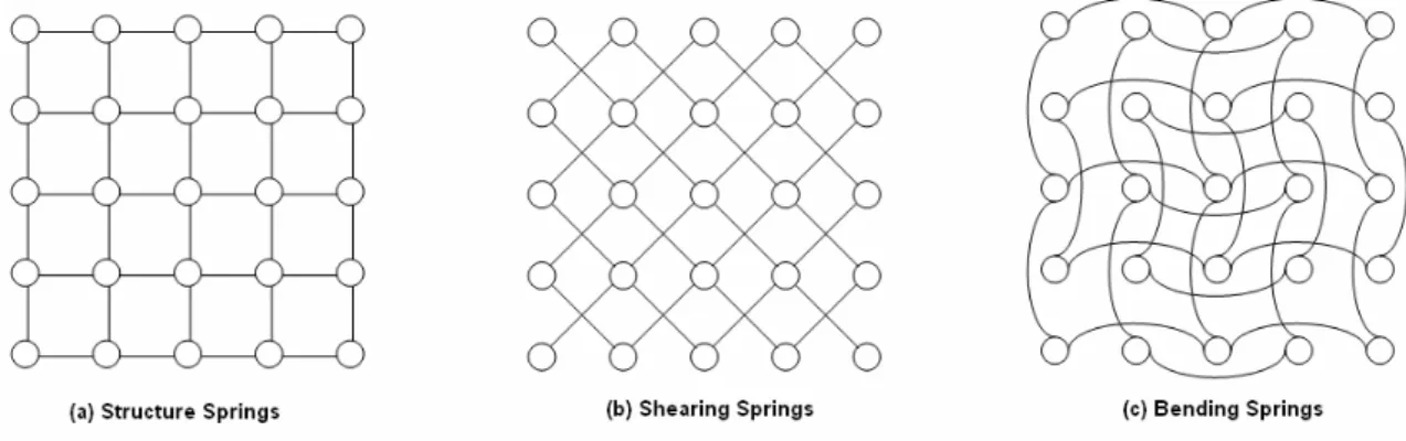
As shown in Fig 4.4, structural springs (Fig 4.4 (a)) are created between each pair of horizontal and vertical particle neighbors to resist stretching and compression of the cloth with very high spring coefficients; shearing springs (Fig 4.4 (b)) are used to make sure that cloth does not shear and spring coefficients are usually set lesser than those of structural springs; and finally bending springs (Fig 4.4 (c)) are created for preventing sharp ridges from cloth while folded. OpenTissue system [22] proposed a more general structure for unstructured mesh such as ordinary mesh. It constructs structural springs with first neighbors of each particle, and connects second, third, or more further neighbors as shearing and bending force as following Fig 4.5.

Figure 4.4: Structural, shearing, bending springs for rectangular cloth

Every spring force is governed by Hooks Law

(

)

(

)

where k is spring coefficient constant, s l=ra −rbis the vector connecting two

particle, l&=v_a −v_b is the related velocity of the spring, R is the rest length and k _d

is the damping coefficient.

4.2.2 Data Structure For Collision

To avoid full collision test for every particle and rigid object, a broad-phase collision detection strategy is required in order to reduce unnecessary testing pair. One major and efficient strategy is Bounding Volume Hierarchy. Among many bounding volume hierarchy strategies such as OBB, it appears that axis-aligned bounding box hierarchy performs better than other bounding volumes method for a highly deformable object such as cloth. It is because of its facility and efficiency in updating hierarchies.

Compare to original testing complexity of n, by applying AABB the complexity can be reduced to O(n) for bottom-up updating and O(log(n)) for testing. Although total complexity remains O(n) in the worst case, it is still useful if testing process is much more complicated than update process. Moreover, updating time can be reduced by canceling updating sometime and enlarge the BVH under the assumption of

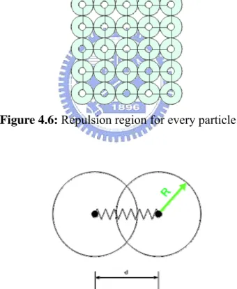
Beside BVH, repulsion force is usually applied before penetration occurred. The repulsion region can be a spherical area around a particle or a given thickness for each triangle. Jansson et al. [17] treated such repulsion as spring force around particles. When two particles move within a nominal distance, a spring is created to push each other away (Fig 4.6, Fig 4.7). With delicate spring constant, this repulsive force can exactly prevent objects from being collided, though constant assignment can be an important issue. Bridon et al. mentioned in [7] that repulsion can reduce the number of collision but cannot guarantee no penetration so that advanced geometric collision method is required.

Figure 4.6: Repulsion region for every particle

Figure 4.7: Spring applied while particles move within nominal distance

However, in this thesis repulsion is used for a collision alleviation method which will be described in detail in chapter 5. To combine this area with bounding volume, bounding boxes can be enlarge a little to cover this repulsion area so that bounding box can also used to detect the repulsion region intersection.

4.3 Numerical Integrator

Numerical integration is important in this thesis since contact force is estimated by Newton’s Laws. However, preventing from calculation burden, a simple explicit integration method can be applied, such as Eular Method for its easy implementation, Verlet Method for its stability or higher-order Runge-Kutta Method for its lesser error. Eular Method: ⎩ ⎨ ⎧ Δ + = Δ + = + + t v x x t a v v n n n n n 1 1 _(4.13) Verlet Method: 2 1 1 (2 f)x (1 f)x a t x_n+ = − _n − − _n− + Δ (4.14)

Fourth-order Runge-Kutta Method:

⎪ ⎪ ⎪ ⎪ ⎪ ⎩ ⎪ ⎪ ⎪ ⎪ ⎪ ⎨ ⎧ Δ + Δ + = Δ + Δ + = Δ + Δ + = = + + + Δ + = = = ′ + ) , ( ) 2 , 2 ( ) 2 , 2 ( ) , ( ) 3 2 ( 6 ) ( ), , ( 3 2 2 2 1 2 1 4 3 2 1 1 0 0 tk y t t f k k t y t t f k k t y t t f k y t f k k k k k t x x x t x x t f x n n n n n n n n n n (4.15)

Method proposed in this thesis is suitable and stable for any integration scheme so that the selection of integration method can be regarded as a performance/ accuracy tradeoff.

Chapter 5

Collision Detection and Response

As mentioned in [7], collision scheme is better divided into two phases: first avoid penetration and then resolve contact after collision actually happens. In this thesis, it is divided into two phases also: first prevent and alleviate collision and then resolve contact with explicit method.

5.1 Collision

5.1.1 Phase 1: Collision Avoidance and Alleviation

The main purpose of phase 1 is to partially avoid some collision and moreover prevent drastic collision before penetration. Usually a repulsive region around the cloth is used in this phase and repulsive force occurs while particles move within the region. A force-based repulsion method is very useful to prevent a number of particle collisions with moderate time interval and dedicate particle velocity. However, this kind of method can be over/under-reacted when objects collide with high speed. Moreover, the force can not easily simulate an inelastic and smooth contact, for example, an interaction between rigid object and cloth.

with a soft thick shell. When two objects move closer, the soft shell will produce a repulsive force to keep objects in distance. The repulsive force is usually modeled as a spring force. This is absolutely reasonable since the stiffness of this soft shell can tuned by spring constant Ks. That is, a high Ks id for a stiff shell and a low Ks is for a soft one. The elasticity can be tuned by spring constant while approaching and leaving such as k_leave =εk_approach, while ε is 1 for perfect elastic collision and 0 for completely

inelastic. For a continuous time domain case in real world, contact problem can illustrate as following Fig 5.1.

Figure 5.1: Collision sequences for real case.

In Fig 5.1(a), two particles start to move forward each other. Then approach and start to compress the spring in Fig 5.1(b) until two particles have the same velocity (system velocity) and spring is maximized compressed in Fig 5.1(c). Afterward, spring pushes two particles away in Fig 5.1(d)(e). However, this is a case in

over-pressed situation may occur as following Fig 5.2 shows

Figure 5.2: Problems for discrete time step

In the case in Fig 5.2(a), spring between particles is over compressed over a time interval. If the spring constant is high, the spring may produce a over-reacted response for each object. Or even, with an insufficient spring constant, particle may still collide to each other. These problems happen related to the time interval and the velocity of each object.

Force-based repulsion is usually used in simulation with dynamic deformable object like cloth and a static or pre-animated rigid object that the position and velocity cannot be changed by forces during simulation. However, the reaction is sensitive to time interval, spring constant and even the relative velocity of each particle.

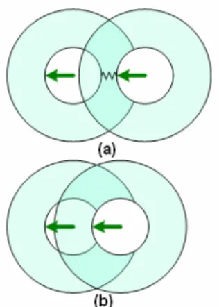
Since force cannot completely avoid collision, this region can be used to avoid drastic collision. Drastic collision can be situations which objects approaches in high velocity or time interval is not small enough to prevent large penetration from happening. Large penetration may cause problems while resolving contact. One of the problems is shown in Fig 5.3 which the object completely moves though the cloths in the next time step. So rather than applying force, it is better directly using a simple

velocity constraint to alleviate collision. To simplify the velocity constraint, two assumptions are made in this thesis. First, a smooth collision between cloth and rigid body is completely inelastic. Second, mass of particles on cloth is much lesser than that of rigid body. These assumptions make sense in real cases and collision can be simplified as Fig 5.4.

Figure 5.3: Problem for drastic collision

Figure 5.4: Inelastic collision between objects with asymmetric mass

rigid object enters into the repulsion region of a particle, the velocity of the particle is modified closer to the system velocity when the rigid object moves nearer. System velocity can calculated as following formula.

_⎟⎟ ⎠ ⎞ ⎜ ⎜ ⎝ ⎛ + + = r p r r p p s m m v m v m v (5.1)

mp, vp are the mass and velocity of particle and mr, vr are those of rigid object. While

mp is much lesser than mr, system velocity vs is approximated to vr.under the second

assumption. Therefore, the velocity of particle is constraint to the distance to rigid object and velocity of the contact point on rigid object when rigid object enters into the repulsion region.

Figure 5.5: Rigid object entered repulsion region of a particle

As figured in Fig 5.5, a rigid object with velocity of vr and angular velocity of ω

enters the repulsion region of particle. And the closest point from particle to the rigid object is pc with distance of d. If we regard repulsive force as a spring, the

post-velocity of particle is a function of d, vp, vr,

v′p = f(d,vp,vr), (5.2)

⎪⎩ ⎪ ⎨ ⎧ + = ′ + ′ = + + + = + ′ + ′ = + s r p r r p p r r p p s r p r r p p r r p p v m m v m v m v m v m kR v m m kd v m v m v m v m ) ( 2 1 ) ( 2 1 2 1 2 1 2 1 2 1 2 1 2 2 2 2 2 2 2 .(5.3) For a given a constant repulsion region radius R, spring constant k should be a function of vp and vr. Because it will be complicated and inefficient to solve v′ , we p

simple formulate the velocity of the particle in an interpolation term,

v′p =αvp +(1−α)vc (5.4)

while vc is the velocity of the contact point.

v_c =v_r +ω×(p_c−p_r)

α is a function of distance d and the value is limited within 0 to 1, 0 for d=0 and 1 for

d=R. It can be formulated as a linear function

R d = α , (5.5) or a polynomial term R d R d 2 2 2 + − = α . (5.6)

And the information pc and d of can be easily gained from distance map for the rigid

object.

This method partially avoids collision, stabilizes the system and prevents drastic collision efficiently. Moreover, the effect is similar to air floating between cloth and rigid object and produces a visual plausible interaction. This method can apply for not only a dynamic rigid object but also an animated one such as a character.

the force that pushed it. This is what phase 2 for.

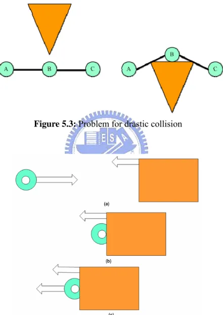
Traditionally, a penalty-based method adds a spring to particle and surface of rigid object. This method is very trivial, but it will be a pain to set a moderate spring constant or the force may not push the particle out. This happens frequently when rigid object is chasing the particle or there are other forces acting on the particle such as gravity.

Figure 5.6: Rigid object chasing a particle

In the case of Fig 5.6, even the velocity of particle increased by spring force, it could not escape from rigid body. If the rigid object has acceleration toward particle, the problem will get worse.

Figure 5.7: The gravity to particle is greater than the spring force

Fig 5.7 illustrates a problem when there are other forces acting on particle. Not only gravity but also the spring force from mass-spring system will resist the penalty force.

Since force-base method is unreliable, it is practical to simply move the particle out of rigid object. This move-out procedure is often called projection. The projection changes the velocity of the particle, and the impulse can be calculated to estimate the constraint force that rigid object acts on particle. This is widely used in constraint-based method. However, calculation of constraint force may require a linear solver such as F=KΔv while K can be a large matrix for an implicit

integration method. This will be a burden for a complicated model such as cloth. That is, an explicit estimation of the contact force can be a nice candidate considering the performance.

So in phase 2, particle is simply projected out of rigid object. The information for the projection can be easily found from the distance map.

Figure 5.8: Projection for a penetrated particle

In Fig 5.8(a), a particle penetrated a rigid object with a depth of d and normal of

n, and then be projected out with these information in Fig 5.8(b).

Figure 5.9: Problem for projection

When the rigid object becomes more complicate or the penetration depth is extremely large, the projection may have problems which may cause system unstable. For example in Fig 5.9, these are three sequential time steps. Particles are first moved by forces to a new position which is represented with transparent color and are then projected out of rigid body. Notice that particles A, C and D oscillate around rigid body. The oscillation may diverge when spring constant is large or the projection

method is not proper. However, the vibration can be alleviated by the method used in phase 1 because we limit the velocity of particles around the rigid body.

5.2 Contact Force

Rather than impulse-based methods, force-based methods are easier to couple two system in different mechanism because interaction can be model as a force applied to each objects. After a particle is projected out of the rigid object, the particle should also push the rigid object back. This is completely based on the Newton’s third law: for every action there is an equal and opposite reaction. Then the magnitude and direction of the contact force should be calculated. There are three explicit methods to estimate the contact force.

First method is very trivial. It re-calculates the composition of forces for the particle after projecting and uses the sub-force which normal to the contact face as the contact force. As shown in Fig 5.10, F is the composition of forces such as spring force from mass-spring system, gravity, friction or other external force. If nˆ is the

normal vector of the contact face, sub-force F⊥ can be calculated by following

equation.

F_⊥ =

(

)

Then F⊥ is used as a contact force acting on the rigid object. This estimation is simple

but inaccurate because it does not consider the change in velocity of the particle. However, this estimation actually works for a coarse contact resolution.

Figure 5.10: Sub-force F is used as contact force

The second method takes velocity into consideration. In physics, energy transfers from one to another by a force. After projecting the particle, the kinetic energy of the particle may be changed, either gained or lost. If an external work W acts upon this particle, it causes the kinetic energy of particle to change from Ek1 to Ek2.

_{2 1 2 1} 2 1 2 1 mv mv E E E W =Δ k = k − k = − (5.8)

If this external work is done by an external force along a path, the work can be defined:

=

∫

C

C F ds

W v v (5.9)

where C is the path or curve traversed by the object, Fv is the force vector and sv is the position vector. Force can be assumed constant and path can be assumed to be a line in discretized time step simulation so that the work can be simplified to:

W =Fv⋅dv (5.10)

where dv is the movement of the particle in this time interval.

As shown in Fig 5.11, the particle moves from outside to inside of the rigid object, and then is projected out of the rigid object. First from Fig 5.11(a) to Fig 5.11(b), the velocity of the particle changes from vn to vtemp by external forces such as spring force and gravity except contact force. Because of the projection, the particle is moved out of rigid object and velocity is modified to the velocity of rigid object on the contact point. In conclusion, the velocity of particle changes from vn to vc by composition of forces, including contact force, working along a distance of d. The energy equation can be written as following.

⎪ ⎪ ⎩ ⎪⎪ ⎨ ⎧ = ⋅ − ⋅ = = − + + + =

∫

Simply speaking, the sub-force of Fall which is parallel to d changes the kinetic energy of the particle and the sub-force of Fall which is perpendicular to d should be zero. Base on these equations the contact force Fc can be calculated. However, this method underestimates the contact force in a situation illustrated in Fig 5.12. This property which comes from the scalar equation is inaccurate but can prevent system from divergence.

which it acts.

J =

∫

So that the equations used in the second method is rewritten. ⎪⎩ ⎪ ⎨ ⎧ Δ = = − + + + =

∫

The contact force can be applied not only after penetration but also before. The change of velocity in phase 1 can regard as a repulsion force which acts not only to particle but also to rigid body. However, energy-based method cannot estimate contact force in phase because there is no displacement. So we can combine impulse-based method in phase 1 to calculate the repulsion force.

Three methods proposed in the thesis are completely explicit and require only vector operator. Therefore, they largely reduce the computational burden of traditional constraint based methods. However, latter two methods sometimes produce force with noise in direction and may produce strange torque to the rigid object. The problem can be solved by only apply the sub-force which parallels to the normal of the contact point.

Chapter 6

Implementation and Result

In this chapter, the full algorithm used in this paper is presented in the first section. In the second chapter, we demonstrate the results in different situation. We will show the result of simulation which only applies phase 1. In this case, an obvious result for collision avoidance method can be observed. Then we will show the results of single rigid body interacting with cloth, and then the result for multiple rigid bodies. Finally in the last section, we will discuss about the limitation of our method.

6.1 Implementation

In Figure 5.1, we outline the entire algorithm for simulating rigid body and cloth in contact. Note that in step 5, distance field functionD

( )

signed distanced and a normal directionnˆ. The function can be a formula for simple

model or a volume texture pre-computed in step 1. d and nˆ can be stored in

RGBA of a texel and d can be normalize within 0 to 1. With some branching factor,

the full algorithm is potentially suited for parallel implementation. Every particle motion and contact force can be simulated independently by GPU textures. And the algorithm can exploit the efficiency of SIMD hardware.

PRE-COMPUTATION

1. Compute distance field as a volume texture.. COLLISION-FREE UPDATE

2. Evaluate forces.

3. Move rigid objects and cloth by chosen integration method. COLLISION DETECTION

4. Execute broad-phase collision detection such as multi-resolution hash table space.

5. Execute narrow-phase collision detection by testing particle position with distance field d,nˆ =D(xv_p)

COLLISION RESPONSE

6. If particle is near to rigid body surface within repulsion region, apply phase 1 to modify the velocity of particle d > −C_rep → vv′_p = αvv_p + (1−α)vv_c

and calculate contact force to apply on rigid body.

7. If particle penetrates into rigid body, project particle out

c p p v v n d x x v v v v = ′ + ′ = ′ ˆ and calculate contact force to apply on rigid body.

8. Repeats steps 2 to 7 for next time step

Figure 6.1: Summary of the Simulation Algorithm

6.2 Result

We have executed our experimentation on a dual cores 1.66 GHz Pentium4 processor with an ATI X1600 graphic card. We use Open Dynamics Engine (ODE) library to simulate rigid body dynamics and render results with Microsoft DirectX 9.0. And all demonstrations are implemented in C++. The cloth in our demonstrations is constructed with 50×80 particles ordered in grids and the simulation time interval is 0.01 seconds per time step.

First of all, an exaggerated example is shown in Fig 6.2. The sphere radius is 3.0 and the radius of the repulsion region around particle is set to 5.0. In Fig 6.2(b) rigid object is within the repulsion region so that the velocity of some particle is slightly changed. And in Fig 6.2(e) the rigid object finally reaches the cloth and the velocity of contact particle is nearly the same to the velocity of the contact point of rigid body. Although this is completely unrealistic, the effect of the repulsion region can be clearly observed. However, we usually set the radius of repulsion region to 1.0.

In Fig 6.3, we compare the situation of applying repulsion or not. In Fig 6.3(a), we use collision alleviation and produce a smooth contact. And in Fig 6.3(b), we close the repulsion effect, and then surface of cloth is obviously vibrating. Moreover, an unstable situation like Fig 6.3(c) happens more frequently with repulsion effect. These cases use the same parameters but the former one applies repulsion while the latter ones do not.

Next, we show the case that the rigid body will not be affected by the cloth in Fig 6.3. This is an example for some pre-animated objects such as character model or for a rigid body with extremely high weight. With the reinforcement of collision alleviation method in phase 1, the projection which moves particle out of rigid body can be smooth and stable. The rigid body is a brick-shaped object which falls from the upper side of the cloth in Fig 6.4 (a). It reaches the floor in Fig 6.4(b) and the cloth is drawn from the bottom of the object in Fig 6.4(c).

In the third demonstration, we compare the contact force which is estimated by different kind of method. The initial position is shown in Fig 6.5(a) and a series of

slightly different in direction and degree of the contact force. Energy-based method in Fig 6.5(d) underestimates the contact force in some situations so that the highest position is lesser than others while subforce-based method in Fig 6.5(b) overestimates contact force so that results in a higher position.

Finally, we show a multiple rigid body interacting with cloth in Fig 6.6. The size, the shape, initial position and initial velocity are randomly assigned. In Fig 6.6(a)(b)(c), the particles on the four corners of the cloth are fixed and then is released after Fig 6.6(d). Moreover, we analysis the relationship between number of objects and time used for simulation in seconds by incrementally adding an object into the system. As shown in Fig 6.7, the simulation time grows linearly while the number of object increases. According to the result we can conclude that the time cost for an object in one simulation step is about 0.000208 second. That is, we can simulate 80 objects simultaneously in a frequency of 60 simulation steps per second and may produce a runtime simulation.

(a) (b)

(c) (d)

(e) (f)

(a)

(b)

(c)

(a) (b)

(c) (d)

(e) (f)

(a) Initial position

(b) Subforce-based method

(c) Impulse-based method

(d) Energy-based method

(a) (b)

(c) (d)

(e) (f)

Figure 6.7: Relationship between number of object and time used for simulation 0 0.002 0.004 0.006 0.008 0.01 0.012 1 4 7 10 13 16 19 22 25 28 31 34 37 40 43 46 49 52 number of object sec on ds p er si m ul at io n

Chapter 7

Conclusion and Future Work

In this thesis, we introduced a collision scheme for the interaction between rigid body and cloth. First, we partially avoid some collision in phase 1 by modified the velocity of particles when cloth and rigid body moving close. This method which also prevents drastic collision provides a smooth and stable contact for cloth and rigid body. Moreover, it prevents unstable divergence of the system which applies explicit method in phase 2. In phase 2, we exploit distance field to efficiently project penetrated particle and explicitly estimate the contact force. The simplified method can largely reduce the time wasted in contact resolution. We sacrifice a little accuracy but produce a stable, plausible and runtime simulation which is useful in game industry.

However, we did not consider friction in this thesis which is usually solved with constraint. The explicit method makes it difficult to estimate reasonable friction force. Moreover, the explicit method may cause error direction while estimating contact force. In future work, we would like to extend our scheme to produce friction effect and reduce the error cause by explicitness. Furthermore, we will combine the continuous collision detection methods to deal with an extremely high speed collision.

References

[1] Anitescu, M. and Potra, F. “Formulating dynamic multi-rigid-body contact problems with friction as solvable linear complementary problems”. Nonlinear

Dynamics, pp. 231-247, 1997

[2] Baraff, D. “Analytical methods for dynamic simulation of non-penetrating rigid bodies”. Proceedings of ACM SIGGRAPH, pp.223–232, 1989

[3] Baraff, D. “Coping with friction for nonpenetrating rigid body simulation”.

Computer Graphics 25, 4, pp.31–40, 1991

[4] Baraff, D. “Issues in computing contact forces for non-penetrating rigid bodies”.

Algorithmica 10, pp.292–352, 1993

[5] Baraff, D. and Witkin, A. “Partitioned dynamics”. Tech. Report CMU-RI-TR-

97-33, Robotics Institute, Carnegie Mellon University, 1997.

[6] Baraff, D., Witkin, A. and Kass, M. “Untangling cloth”. Proceedings of ACM

SIGGRAPH, pp.862-870, 2003

[7] Bridson, R., Fedkiw, R. and Anderson, J. “Robust treatment of collisions contact and friction for cloth animation”. Proceedings of ACM SIGGRAPH, pp.594-603, 2002 [8] Erleben, K., Sporring, J., Henriksen, K. and Dohlmann, H. “Physics-based Animation”. Jenifer Niles, 2005

[9] Galoppo, N., Otaduy, M.A., Mecklenburg, P., Gross, M. and Lin, M.C. “Fast simulation of deformable models in contact using dynamic deformation textures”.

Proceedings of the ACM SIGGRAPH/Eurographics symposium on Computer animation, pp.73-82, 2006

[10] Guendelman, E., Bridson, R. and Fedkiw, R. “Nonconvex rigid bodies with stacking”. ACM Transactions on Graphics 22, 3, pp.871–878, 2003

conference on Computer graphics and interactive techniques, pp.299– 308, 1988

[12] Hirota, G., Fisher, S., State, A., Lee, C. and Fuchs, H. “An Implicit finite element method for elastic solids in contact”. In Computer Animation, Seoulm South Korea, 2001

[13] Hirota, G. “An improved finite element contact model for anatomical simulations”. PhD thesis, University of N. Carolina, Chapel Hill, 2002

[14] House, D. H. and Breen, D. “Cloth Modeling and Animation”. A.K. Peters, 2000 [15] Hubbard, P.M. “Interactive collision detection”. Proceeding of the IEEE

Symposium on Research Frontiers in Virtual Reality, pages 24-32, 1993

[16] Ilenkovic, V. J. and Schmidl, H. “Optimization-based animation”. Proceedings of

ACM SIGGRAPH, pp. 37–46, 2001

[17] Jansson, J. and Vergeest, J. S. M. “Combining deformable and rigid body mechanics simulation”. The Visual Computer Journal, pp.280-298, 2003

[18] Mirtich, B. and Canny J. “Impulse-based simulation of rigid bodies”. Symposium

on Interactive 3D Graphics, pp. 181–188, 1995

[19] Moore, M. and Wilhelms, J. “Collision detection and response for computer animation”. Proceedings of ACM SIGGRAPH, pp. 289–298, 1988

[20] O’Brien, J., Zordan, V. and Hodgins, J. “Combining active and passive simulations for secondary motion”. IEEE Computer Graphics and Applications, Vol. 20, No. 4, pp.86-96, 2000

[21] Open Dynamics Engine. Opensource Project, Multibody Dynamics Software, q12.org/ode/.

[22] OpenTissue. http://www.opentissue.org

[24] Pauly, M., Pai, D.K. and Guibas, L.J. “Quasi-rigid objects in contact”.

Proceedings of the 2004 ACM SIGGRAPH/Eurographics symposium on Computer animation, pp.109-119, 2004

[25] Provot, X. “Deformation constraints in a mass-spring model to describe rigid cloth behavior”. Proceedings Graphics Interface, pp. 147-154, 1995

[26] Sauer, J. and Schömer, E. “A constraint-based approach to rigid dynamics for virtual reality application”. ACM Symposium on Virtual Reality Software and

Technology, pp. 153-161, 1998

[27] Stanford bunny, http://graphics.stanford.edu/data/3Dscanrep/

[28] Stewart, D. and Trinkle, J. “An implicit time-stepping scheme for rigid body dynamics with inelastic collision and coulomb friction”. International Journal of

Numerical Methods in Engineering, 1996

[29] Stewart, D. and Trinkle, J. “An implicit time-stepping scheme for rigid body dynamics with coulomb friction”. IEEE International Conference on Robotics and

Automation, pp. 162-169, 2000

[30] Sud, A., Govindaraju, N., Gayle, R. and Manocha, D. “Interactive 3D distance field computation using linear factorization”. Proc. ACM Symposium on Interactive

3D Graphics and Games, pp.117-124, 2006

[31] Terzopoulos, D., Platt, J. C. and Barr, A. H. “Elastically deformable models”. In